Improving Portfolio Selection
Using Option-Implied Volatility and Skewness
∗
Victor DeMiguel‡ Yuliya Plyakha§ Raman Uppal¶ Grigory Vilkov§
This version: June 11, 2012
∗We gratefully acknowledge financial support from Inquire-Europe; however, this article represents
the views of the authors and not of Inquire. We would like to acknowledge detailed feedback from Luca Benzoni, Pascal Maenhout, and Christian Schlag. We received helpful comments and suggestions from Alexander Alekseev, Michael Brandt, Mike Chernov, Engelbert Dockner, Bernard Dumas, Wayne Ferson, Rene Garcia, Lorenzo Garlappi, Nicolae Gˆarleanu, Amit Goyal, Jakub Jurek, Nikunj Kapadia, Ralph Koijen, Lionel Martellini, Vasant Naik, Stavros Panageas, Andrew Patton, Boryana Racheva-Iotova, Marcel Rindisbacher, Paulo Rodrigues, Pedro Santa-Clara, Bernd Scherer, Peter Schotman, George Ski-adopoulos, Luis Viceira, Josef Zechner, and seminar participants at AHL (Man Investments), BlackRock, Goethe University Frankfurt, London School of Economics, University of Mainz, University of Piraeus, University of St. Gallen, Vienna University of Economics and Business Administration, CEPR Euro-pean Summer Symposium on Financial Markets, Duke-UNC Asset Pricing Conference, EDHEC-Risk Seminar on Advanced Portfolio Construction, Financial Econometrics Conference at Toulouse School of Economics, SIFR Conference on Asset Allocation and Pricing in Light of the Recent Financial Crisis, and meetings of the European Finance Association, Western Finance Association, and the Joint Conference of INQUIRE-UK and INQUIRE-Europe 2011.
‡London Business School, 6 Sussex Place, Regent’s Park, London, United Kingdom NW1 4SA; E-mail:
§Goethe University Frankfurt, Finance Department, Gr¨uneburgplatz 1 / Uni-Pf H 25, D-60323
Frank-furt am Main, Germany; Email: [email protected]@vilkov.net.
¶CEPR and Edhec Business School, 10 Fleet Place, Ludgate, London, United Kingdom EC4M 7RB;
Improving Portfolio Selection
Using Option-Implied Volatility and Skewness
This version: June 11, 2012
Abstract
Our objective in this paper is to examine whether one can use option-implied information to improve the selection of mean-variance portfolios with a large number of stocks, and to document which aspects of option-implied informa-tion are most useful for improving their out-of-sample performance. Portfolio performance is measured in terms of volatility, Sharpe ratio, and turnover. Our empirical evidence shows that using option-implied volatility helps to reduce portfolio volatility. Using option-implied correlation does not improve any of the metrics. Using option-implied volatility, risk-premium, and skew-ness to adjust expected returns leads to a substantial improvement in the Sharpe ratio, even after prohibiting shortsales and accounting for transac-tions costs.
Keywords: mean variance, option-implied volatility, variance risk premium, option-implied skewness, portfolio optimization
1
Introduction
To determine the optimal mean-variance portfolio of an investor, one needs to estimate the moments of asset returns, such as means, volatilities, and correlations. Traditionally, historical data on returns have been used to estimate these moments, but researchers have found that portfolios based on sample estimates perform poorly out of sample.1 Several
approaches have been proposed for improving the performance of portfolios based on
historical data.2
In this paper, instead of trying to improve the quality of the moments estimated from historical data, we use forward-looking moments of stock-return distributions that are implied by option prices. The main contribution of our work is to evaluate empir-ically which aspects of option-implied information are particularly useful for improving the out-of-sample performance of portfolios with a large number of stocks. Specifically, we consider option-implied volatility, correlation, skewness, and the risk premium for stochastic volatility, and we obtain these not just from the Black-Scholes model, but also using the model-free approach developed in Bakshi, Kapadia, and Madan (2003).
First, we consider the use of option implied volatilities and correlations to improve out-of-sample performance of mean-variance portfolios invested in only risky stocks. When evaluating the benefits of using option-implied volatilities and correlations, we set ex-pected returns to be the same across all assets so that the results are not confounded by the large errors in estimating expected returns.3 Consequently, the mean-variance portfo-lio reduces to the variance portfoportfo-lio. In addition to considering the minimum-variance portfolio based on the sample cominimum-variance matrix, we consider also the shortsale-constrained minimum-variance portfolio, the minimum-variance portfolio with shrinkage
1For evidence of this poor performance, see DeMiguel, Garlappi, and Uppal (2009), Jacobs, Muller, and Weber (2010), and the references therein.
2These approaches include: imposing a factor structure on returns (Chan, Karceski, and Lakon-ishok, 1999), using data for daily rather than monthly returns (Jagannathan and Ma, 2003), using Bayesian methods (Jobson, Korkie, and Ratti, 1979; Jorion, 1986; P´astor, 2000; Ledoit and Wolf, 2004b), constraining shortsales (Jagannathan and Ma, 2003), constraining the norm of the vector of portfolio weights (DeMiguel, Garlappi, Nogales, and Uppal, 2009), and using stock-return characteristics such as size, book-to-market ratio, and momentum to choose parametric portfolios (Brandt, Santa-Clara, and Valkanov, 2009).
3Jagannathan and Ma (2003, pp. 1652–1653) write that: “The estimation error in the sample mean is so large nothing much is lost in ignoring the mean altogether when no further information about the population mean is available.
of the covariance matrix (as in Ledoit and Wolf (2004a,b)), and the minimum-variance portfolio obtained by assuming all correlations are equal to zero or with correlations set equal to the mean correlation across all asset pairs (as suggested by Elton, Gruber, and Spitzer (2006)). We find that using risk-premium-corrected option-implied volatilities in minimum-variance portfolios improves the out-of-sample volatility by more than 10% compared to the traditional portfolios based on only historical stock-return data, while the changes in the Sharpe ratio are insignificant. Thus, using option-implied volatility allows one to reduce the out-of-sample portfolio volatility significantly.
Next, we examine the use of risk-premium corrected option-implied correlations to improve the performance of minimum-variance portfolios. We find that in most cases option-implied correlations do not lead to any improvement in performance. Our em-pirical results indicate that the gains from using implied correlations are not substantial enough to offset the higher turnover resulting from the increased instability over time of the covariance matrix when it is estimated using option-implied correlations.
Finally, to improve the out-of-sample performance of mean-variance portfolios we consider the use of option-implied volatility, risk premium for stochastic volatility, and option-implied skewness. These characteristics have been shown in the literature to help explain the cross section of expected returns.4 Therefore, it makes sense to explore their
effect in the framework of mean-variance portfolios. Using these characteristics to rank stocks and adjusting by a scaling factor the expected returns of the stocks, or using these characteristics with the parametric-portfolio methodology of Brandt, Santa-Clara, and Valkanov (2009), leads to a substantial improvement in the Sharpe ratio, even after prohibiting shortsales and accounting for transactions costs.
We conclude this introduction by discussing the relation of our work to the exist-ing literature. The idea that option prices contain information about future moments of asset returns has been understood ever since the work of Black and Scholes (1973) and Merton (1973); Poon and Granger (2005) provide a comprehensive survey of this
4For instance, Bollerslev, Tauchen, and Zhou (2009) have documented a positive relation between the variance risk premium and future returns. Bali and Hovakimian (2009) and Goyal and Saretto (2009) show that stocks with a large spread between Black-Scholes implied volatility and realized volatility tend to outperform those with low spreads. Bali and Hovakimian (2009), Xing, Zhang, and Zhao (2010), and Cremers and Weinbaum (2010) find a positive relation between various measures of option-implied skewness and future stock returns.
literature. The focus of our work is to investigate how the information implied by op-tion prices can be used to improve portfolio selecop-tion. There are two other papers that study this. The first, by A¨ıt-Sahalia and Brandt (2008), uses option-implied state prices to solve for the intertemporal consumption and portfolio choice problem, using the Cox and Huang (1989) martingale representation formulation, rather than the Merton (1971) dynamic-programming formulation; however, its focus is not on finding the optimal port-folio with superior out-of-sample performance. The second, by Kostakis, Panigirtzoglou, and Skiadopoulos (2011), studies the asset-allocation problem of allocating wealth be-tween the S&P500 index and a riskless asset. This paper finds that the out-of-sample performance of the portfolio based on the return distribution inferred from option prices is better than that of a portfolio based on the historical distribution. However, there is an important difference between this work and ours: rather than considering the problem of how to allocate wealth between the S&P500 index and the riskfree asset, we consider the portfolio-selection problem of allocating wealth across a large number of individual stocks. It is not clear how one would extend the methodology of Kostakis, Panigirtzoglou, and Skiadopoulos (2011) to accommodate a large number of risky assets. They also need to make other restrictive assumptions, such as the existence of a representative investor and the completeness of financial markets, which are not required in our analysis.
The rest of the paper is organized as follows. In Section 2, we describe the data on stocks and options that we use. In Section 3, we explain how we use data on options to predict volatilities, correlations, and expected returns. In Section 4, we describe the construction of the various portfolios we evaluate along with the benchmark portfolios, and the metrics used to compare the performance of these portfolios. Our main findings about the performance of various portfolios that use option-implied information are given in Section 5. We conclude in Section 6.
2
Data
In this section, we describe the data on stocks and stock options that we use in our study. Our data on stocks are from the Center for Research in Security Prices (CRSP). To implement the parametric-portfolio methodology, we also use data from Compustat. Our
data for options are from IvyDB (OptionMetrics). Our sample period is from January 1996 to October 2010.5
2.1
Data on Stock Returns and Stock Characteristics
We study stocks that are in the S&P500 index at any time during our sample period. The daily stock returns of the S&P500 constituents are from the daily file of the CRSP, and we have in our sample a total of 3,986 trading days.6 Counting by CRSP identifiers (PERMNO), we have data for a maximum of 961 stocks. Out of these 961 stocks, there are 143 stocks for which implied volatilities are available for the entire time series. For robustness, we consider two samples in our analysis. The first, which we label “Sample 1,” consists of the 143 stocks for which the data are available for all dates. The second, “Sample 2,” consists of all the stocks that are part of the S&P500 index on that day and which have no missing data on that day (such as prices of options on the same underlying for a given maturity and across different strikes that are need to compute model-free implied volatilities), which means that the second sample has a variable number of stocks; on average, this sample has about 400 stocks at each point in time.7
We measure size (market value of equity) as the price of the stock per share multiplied by shares outstanding; both variables are obtained from the CRSP database. For mea-suring value or book-to-market (BTM) characteristic, we use the Compustat Quarterly Fundamentals file. The twelve-month momentum (MOM) characteristic is measured for each day t using daily returns data from CRSP as the cumulative return from day t−21−251 to day t−21.8
5We carry out all the tests included in the manuscript also for the pre-crisis period from January 1996 to December 2007, and the crisis period from January 2008 to June 2009 (identified as a recession by the NBER). The main insights of our analysis do not change with the choice of sample period.
6We also use high-frequencyintradaystock-price data consisting of transaction prices for the S&P500 constituents from the NYSE’s Trades-And-Quotes database; the results for these data are very similar to those using daily data.
7The main difference between Sample 1 and Sample 2 is that for estimating the parameters of the covariance matrix for Sample 2, which has more stocks, one needs a longer estimation window. Thus, while the estimation window for Sample 1 is 250 trading days, for Sample 2 it is 750 days. As a result of the longer estimation window, the weights are relatively more stable over time for Sample 2. On the other hand, because the covariance matrix for Sample 2 is of a larger dimension, its condition number is different from that of the covariance matrix for Sample 1.
8To get better distributional properties of the constructed characteristics, we take the logarithm of size and value characteristics. In order to prepare these characteristics so that they can be used to compute the parametric portfolio weights, we also winsorize the characteristics by assigning the value of
2.2
Data on Stock Options
For stock options we use IvyDB that contains data on all U.S.-listed index and equity options, most of which are American. We use the volatility surface file, which contains a smoothed implied-volatility surface for a range of standard maturities and a set of option delta points. From the surface file we select the out-of-the-money implied volatilities for calls and puts (we take implied volatilities for calls with deltas smaller or equal to 0.5, and implied volatilities for puts with deltas bigger than−0.5) for a maturity of 30 days.9 For
each date, underlying stock, and time to maturity, we have 13 implied volatilities from the surface data, which are used to calculate the moments of the risk-neutral distribution. Some of the option-based characteristics also use the parametric Black-Scholes implied volatilities for at-the-money options. We compute the at-the-money volatility as the average volatility for a put and a call with absolute delta level equal to 0.5.
3
Option-Implied Information
In this section, we explain how we compute the option-implied moments that we use for portfolio selection; we compare the ability of option-implied moments and the historical moments to forecast the actual realized moments. We consider the following measures: (i) model-free option-implied volatility; (ii) the volatility risk premium, measured as the spread between realized and Black-Scholes option-implied volatility; (iii) option-implied correlation; (iv) model-free option-implied skewness; and (v) a proxy for skewness, mea-sured as the spread between the Black-Scholes implied volatility obtained from calls and that from puts.
the 3rd percentile to all values below the 3rd percentile and do the same for values higher than the 97th percentile. Finally, we normalize all characteristics to have zero mean and unit standard deviation.
9The use of out-of-the-money options is standard in this literature; see, for instance, Bakshi, Kapadia, and Madan (2003) and Carr and Wu (2009). The reason for selecting options that are out of the money is that it reduces the effect of the premium for early exercise of American options.
3.1
Predicting Volatilities Using Options
When option prices are available, an intuitive first step is to use this information to back out implied volatilities and use them to predict volatility.10 In contrast to the
model-specific Black and Scholes (1973) implied volatility, we use for this purpose themodel-free implied volatility (MFIV), which represents a nonparametric estimate of the risk-neutral expected stock-return volatility until the option’s expiration. It subsumes information in the whole Black-Scholes implied volatility smile (Vanden (2008)) and is expected to predict the realized volatility better than the Black-Scholes volatility. We compute MFIV as the square root of the variance contract of Bakshi, Kapadia, and Madan (2003), as explained below.
Let S(t) be the stock price at time t, R(t, τ) ≡ lnS(t +τ)− lnS(t) the τ-period log return, and r the risk-free interest rate. Let V(t, τ) ≡ E∗
t{e
−rτR(t, τ)2}, W(t, τ) ≡
E∗t{e
−rτR(t, τ)3}, andX(t, τ)≡
E∗t{e
−rτR(t, τ)4}represent the fair value of the variance,
cubic, and quartic contracts, respectively, as defined in Bakshi, Kapadia, and Madan (2003). Define µ(t, τ) =erτ−1− e rτ 2 V(t, τ)− erτ 6 W(t, τ)− erτ 24X(t, τ). Then, the τ-period model-free implied volatility (MFIV) can be calculated as
MFIV(t, τ) = V(t, τ)1/2, (1)
and theτ-period model-free implied skewness (MFIS) as
MFIS(t, τ) = e
rτW(t, τ)−3µ(t, τ)erτV(t, τ) + 2(µ(t, τ))3
(erτV(t, τ)−(µ(t, τ))2)32
. (2)
To compute the integrals that give the values of the variance, cubic, and quartic contracts precisely, we need a continuum of option prices. We discretize the respective integrals and approximate them using the available options. As mentioned earlier, we
10Note that our objective isonly to show that the option-implied moments provide better forecasts than the estimators based on historical sample data, rather than to demonstrate that option-implied moments provide thebest forecasts of future volatility and correlations. There is a very large literature on forecasting stock-return volatility and correlations; see, for instance, the survey article by Andersen, Bollerslev, and Diebold (2009).
normally have 13 out-of-the-money call and put implied volatilities for each maturity. Using cubic splines, we interpolate them inside the available moneyness range, and ex-trapolate using the last known (boundary for each side) value to fill in a total of 1001 grid points in the moneyness range from 1/3 to 3. Then we calculate the option prices from the interpolated volatilities using the known interest rate for a given maturity and use these prices to compute the model-free implied volatility and model-free implied skewness as in (1) and (2), respectively.
However, what we need for portfolio selection is not the risk-neutral implied volatility of stock returns but the expected volatility under the objective distribution. We now explain how to use information in the model-free implied volatility in order to get the volatility under the objective measure.
The implied volatility differs from the expected volatility under the true measure by the volatility risk premium. Bollerslev, Gibson, and Zhou (2004), Carr and Wu (2009), and others have shown that one can use realized volatility (RV), instead of the expected volatility, to estimate the volatility risk premium. Assuming that the magnitude of the volatility risk premium is proportional to the level of volatility under the true probability measure, we estimate the monthly historical volatility risk premium adjustment (HVRP) for a particular stock as the ratio of average monthly implied and realized volatilities for that stock for the past T + ∆t trading days:11
HVRPt= Pt−∆t i=t−T−∆t+1MFIVi,i+∆t Pt−∆t i=t−T−∆t+1RVi,i+∆t . (3)
In our analysis, we estimate the historical volatility risk premium adjustment on each day over the past year (−272 days to −21 days) using the model-free implied volatility and realized volatility from daily returns, each measured over 21 trading days and each annualized appropriately. Then, assuming that in the next period, fromt tot+ ∆t, the prevailing volatility risk premium will be well approximated by the historical volatility risk premium in (3), one can obtain the prediction of the future realized volatility, RVct,
11Note that because HVRP
tis calculated as the ratio of the average MFIVi,i+∆tand RVi,i+∆t, both
which we call therisk-premium-corrected implied volatility:12 c RVt,t+∆t= MFIVt,t+∆t HVRPt .
We now wish to confirm the intuition that risk-premium-corrected implied volatility is better than historical volatility at predicting realized volatility. To do this, we consider as a predictor, first historical volatility and then risk-premium-corrected implied volatility, for the monthly realized volatility from daily returns for each stock. We compare the performance of each predictor in terms of root mean squared error (RMSE) and mean prediction error (ME). We find that the average RMSE in Sample 1 for the risk-premium-corrected implied volatility is 0.1274, which is smaller than the RMSE of 0.1671 for historical daily volatility. The ME for both predictors is negative, indicating that on average both measures are biased upwards with respect to the realized volatility; however, the ME of −0.0047 for the risk-premium-corrected implied volatility is one order of magnitude smaller than the ME of−0.0185 for historical volatility.
3.2
Predicting Correlations Using Options
The second piece of option-implied information that we consider is implied correlation, and, because for the portfolio optimization we need the correlation under the objective
measure, we discuss directly how to obtain option-implied correlation corrected for the risk premium.
If a portfolio is composed of N individual stocks with weights wi, i = {1, . . . , N},
we can write the variance of the portfolio p under the objective (physical) probability measureP as: σp,tP 2 = N X i=1 w2i σPi,t2+ N X i=1 N X j6=i wiwjσi,tPσ P j,tρ P ij,t. (4)
Assume that we have estimated the expectation of the future volatilities of the portfolio
b
σP
p,t and of its componentsσb
P
i,t, and we want to estimate the set of expected correlations
12Another method for obtaining the predictor of future realized volatility is to use a modified version of the heterogeneous autoregressive model of realized volatility proposed by Corsi (2009). We find that the root mean squared error and mean prediction error with this measure are larger than those using the approach we adopt.
b
σP
ij,t that turn Equation (4) into identity. Once we substitute into (4) the expected
volatilities, we have one equation with N×(N −1)/2 unknown correlations, ρbP
ij,t. Thus,
to compute all pairwise correlations we need to make some identifying assumptions. We use the approach proposed in Buss and Vilkov (2011), who compute a hetero-geneous implied-correlation matrix, where all pairwise correlations are allowed to be different.13 Under their approach, the expected correlation is assumed to differ from
the historical correlation by a fixed proportion ψ of the distance between the historical correlation and the maximum correlation of one:
ρPij,t−ρbPij,t=ψt(1−ρPij,t),
which implies that
b
ρPij,t=ρPij,t−ψt(1−ρPij,t). (5)
When we substitute this into Equation (4) above, we get:
b σM,tP 2 =X i X j wiwjbσ P i,tσb P j,t ρ P ij,t−ψt(1−ρPij,t) ,
from which one can derive an explicit expression for the parameter ψt:
ψt=− (bσM,tP )2−P i P jwiwjσb P i,tσb P j,tρPij,t P i P jwiwjbσ P i,tbσ P j,t(1−ρPij,t) ,
and then the expected correlations ρbPij,t from equation (5). Thus, we construct the “het-erogenous” implied-correlation matrix corrected for the risk premium, inferred from ex-pected index and individual volatilities, which contains the up-to-date market perception of future correlation under the true measure.
To determine whether option-implied correlation is superior to historical correlation at predicting realized correlation, we compute the RMSE and ME for these two predictors of the 21-days realized correlation. In both Sample 1 and 2, we find that the RMSE for historical correlation is about 0.25 and is slightly smaller than the RMSE of 0.26 for the option-implied correlation; note, however, that the RMSE for both predictors is only
13An alternative approach is to compute homogeneous implied correlations, where all pairwise corre-lations are assumed to be the same: ρbPij,t=ρbPt,∀i6=j. This is the approach used in Driessen, Maenhout,
and Vilkov (2009). We considered also this approach, but the portfolios constructed using this approach perform worse than those when correlations are allowed to vary across assets.
slightly smaller than the average realized correlation of 0.29 for our sample, implying that there is very little predictability. For Sample 1, the ME of 0.0039 for historical correlation is of the same order of magnitude as the ME of−0.0068 for implied correlation, while for Sample 2 the ME of 0.0342 for historical correlation is one order of magnitude greater than the ME of 0.0071 for implied correlation.
3.3
Explaining Returns Using Options
There are four option-based quantities that we use to explain returns in the cross-section; the first one is option-implied volatility, the next is based on the risk premium for stochas-tic volatility, and the last two are based on option-implied skewness. We first describe each of these quantities and then test empirically if these characteristics have significant power to explain the cross-section of returns in our samples.
The first option-based characteristic we use is option-implied volatility. Ang, Bali, and Cakici (2010) show that stocks with high current levels of option-implied volatility earn in the next periods higher returns than stocks with low levels of implied volatility. To maximize the information content of the option-implied volatility proxy, we use the model-free implied volatility (MFIV) described in Section 3.1.
The second option-based characteristic we use is the variance risk premium, which is defined as the difference between risk-neutral (implied) and objective (expected or realized) variances. Previous research (see the papers cited in Footnote 4) documents a positive relation between the variance risk premium and future stock returns. We use the implied-realized volatility spread (IRVS) as a measure of the volatility risk premium. We compute IRVS using the approach in Bali and Hovakimian (2009), as the spread between the Black-Scholes implied volatility averaged across call and put options, and the realized stock-return volatility for the past month (21 trading days).
The third characteristic we consider is option-implied skewness. We use two measures of this. The first, model-free implied skewness (MFIS), as defined in Equation (2), represents a nonparametric estimate of the risk-neutral stock-return skewness.14 Rehman
14For the relation between expected stock returns and skewness measured directly, as opposed to option-implied skewness, see Rubinstein (1973), Kraus and Litzenberger (1976), Harvey and Siddique (2000), and Boyer, Mitton, and Vorkink (2009). For a study of asset allocation that takes into account
and Vilkov (2009) find that stocks with high option-implied skewness outperform stocks with low option-implied skewness.15 The second measure of skewness we consider is the
spread between the Black-Scholes implied volatility for pairs of calls and puts, which is studied in Bali and Hovakimian (2009) and Cremers and Weinbaum (2010). We follow the methodology of Bali and Hovakimian (2009) to compute the call-put volatility spread (CPVS) as the difference between the current Black-Scholes implied volatilities of the one-month at-the-money call and put options.
In order to evaluate if each of these four option-implied measures is useful for ex-plaining the cross-sectional returns for our samples, we examine the returns of long-short decile portfolios for each characteristic separately. The long-short strategies are rebal-anced daily based on the characteristic value at the end of a day, and each portfolio is held for the particular holding period we are considering (one day, one week, or two weeks). In Table 1 we show the annualized returns for each portfolio, along with the p-value, based on the Newey and West (1987) standard errors with a lag equal to the number of overlapping portfolio returns for each holding period. For completeness, we also include in the table standard characteristics such as size (SIZE), book-to-market (BTM), and 12-month momentum (MOM).
Table 1 confirms that the Fama-French characteristics (SIZE and BTM) explain re-turns in the expected direction, while momentum (MOM) is not significant. More inter-estingly, most option-based characteristics lead to significant returns on the long-short decile portfolios. The strongest results—in terms of the magnitude of returns, persis-tence across holding periods, and significance of returns—are for the portfolios based on the two measures of implied skewness, model free implied skewness (MFIS) and the call-put implied volatility spread (CPVS), and for model free implied volatility (MFIV); as expected, high decile stocks outperform the low decile ones for these measures. The
time-variations in risk premia, volatility, correlations, skewness, kurtosis, co-skewness and co-kurtosis measured directly from stock returns, see Guidolin and Timmermann (2008).
15Some researchers (for example, Xing, Zhang, and Zhao (2010)) use as a simple measure of skewness the difference between the implied-volatilities for out-of-the-money put and at-the-money call options. However, that measure does not take into account the whole distribution, but rather just the left tail. Moreover, it is based on only two options and, hence, may be less informative than implied skewness, measured using the entire range of out-of-the money options. Rehman and Vilkov (2009) find that risk-neutral skewness contains information about future stock returns above and beyond that contained in the simple measure of skew.
implied-realized-volatility spread (IRVS) is also positively and significantly related to returns, but at the 10% level.
Looking across the three rebalancing periods, we see that the magnitude of the returns for the option-implied characteristic portfolios decreases as the holding period increases. However, the rate of change of return with the holding period is not the same across characteristics: for example, in Sample 2, for the daily holding, it is the CPVS portfolio that earns the highest return of 86.99% p.a., while for the fortnightly holding period, it is the MFIS portfolio that delivers the highest return of 17.98% p.a. Thus, the various characteristics will lead to different out-of-sample portfolio performance for the daily, weekly, and fortnightly investment horizons that we consider.
4
Portfolio Construction and Performance Metrics
In this section, we explain the construction of the various portfolios we consider and also the metrics used to compare the performance of the benchmark portfolios with that of portfolios based on option-implied information. For robustness, we consider six benchmark portfolios that do not rely on option-implied information.
4.1
Equal-Weighted Portfolio
For the “equal-weighted” (1/N) portfolio, each period one allocates an equal amount of wealth across all N available stocks. The reason for considering this portfolio is that DeMiguel, Garlappi, and Uppal (2009) and Jacobs, Muller, and Weber (2010) show that it performs quite well even though it does not rely on any optimization; for example, the Sharpe ratio of the 1/N portfolio is more than double that of the S&P500 over our sample period.
4.2
Minimum-Variance Portfolios
The mean-variance optimization problem can be written as min
w w >ˆ
Σw−w>µ,ˆ (6)
where w ∈ IRN is the vector of portfolio weights invested in stocks, ˆΣ ∈ IRN×N is the estimated covariance matrix, ˆµ ∈ IRN is the estimated vector of expected returns, and e∈IRN is the vector of ones. The objective in (6) is to minimize the difference between the variance of the portfolio return, w>Σw, and its mean,ˆ w>µ. The constraintˆ w>e = 1 in (7) ensures that the portfolio weights sum to one; we consider the case without the risk-free asset because our objective is to explore how to use option-implied information to select the portfolio of only risky stocks.
In light of our discussion in the introduction about the difficulty in forecasting ex-pected returns, when we are studying the benefits of using option-implied second mo-ments we assume that the expected return for each asset is equal to the grand mean return across all assets. In this case, the mean-variance portfolio problem reduces to finding the portfolio that minimizes the variance of the portfolio return, subject to the constraints that the portfolio weights sum to one. The solution to the resulting minimum-variance
portfolio problem is:
wmin =
ˆ Σ−1e
e>Σˆ−1e. (8)
The covariance matrix ˆΣ in (8) can be decomposed into volatility and correlation matri-ces,
ˆ
Σ = diag(ˆσ) ˆΩ diag(ˆσ), (9)
where diag (ˆσ) is the diagonal matrix with volatilities of the stocks on the diagonal, and ˆ
Ω is the correlation matrix. Thus, to obtain the optimal portfolio weights in (8) based on the sample covariance matrix, there are two quantities that need to be estimated: volatilities (ˆσ) and correlations ( ˆΩ).
In the existing literature, several methods have been proposed to improve the out-of-sample performance of the minimum-variance portfolio based on out-of-sample (co)variances. We consider four approaches. The first is to impose constraints on the portfolio weights, which Jagannathan and Ma (2003) show can lead to substantial gains in performance. Thus, our next benchmark is the “constrained” portfolio, where we compute the shortsale-constrained minimum-variance portfolio weights.
The second approach we consider is the “shrinkage” portfolio, where we compute the minimum-variance portfolio weights after shrinking the covariance matrix. First, the sample covariance matrix for daily data is computed using the same approach that is described above. Then, to shrink the covariance matrix for daily returns, we use the approach in Ledoit and Wolf (2004a,b).
We also consider two other methods proposed in the literature for improving the be-havior of the covariance matrix (see Elton, Gruber, and Spitzer (2006) and the references therein). The first relies on setting all correlations equal to zero so that the covariance matrix contains only estimates of variances. The second relies on setting the correlations equal to the mean of the estimated correlations; we do not report the performance of portfolios based on the second method because they perform worse in terms of all three performance metrics when compared to portfolios obtained from the first method.
4.3
Mean-Variance Portfolios
In the previous section, we assumed that all assets had the same expected return. How-ever, the recent literature on empirical asset pricing (see, for example, the papers cited in Footnote 4) has found that quantities that can be inferred from option prices such as the volatility risk premium and option-implied skewness are useful for predicting returns on stocks. At first sight, one may want to study the effect of using these variables directly in improving the performance of traditional mean-variance portfolios obtained from solving the problem in (6) subject to the constraint in (7). But, it is well known in the literature (see, for example, DeMiguel, Garlappi, and Uppal (2009) and Jacobs, Muller, and Weber (2010)) that the weights of the traditional mean-variance portfolio are very sensitive to errors in estimates of expected returns, and perform poorly out of sample.
Therefore, when evaluating the benefits of using option-based characteristics to form mean-variance portfolios, we use two alternative approaches. In the first approach, we use option-based characteristics to form portfolio deciles, and then adjust the returns of only the top and bottom decile portfolios by a constant factor. In the second approach, we use the ‘parametric-portfolio methodology,” of Brandt, Santa-Clara, and Valkanov (2009), which has been developed to deal with the problem of poor out-of-sample performance of
mean-variance portfolios because of estimation error, and which can be interpreted as a method where the adjustment of stock returns is done in an optimal fashion. We provide details of these two approaches below.
4.3.1 Mean-Variance Portfolios With Characteristic-Adjusted Returns
In the first approach, we assume that the conditional expected return Et[ri,t+1] =µi,t of
stockiat timet can be written as a function of the stock characteristicsk ={1, . . . , K}. More precisely, we specify that
µi,t =µbench,t 1 + K X k=1 δk,txik,t ,
where µbench,t is the expected benchmark return at t (we choose the benchmark return
to the be grand mean return across all stocks), the value of xik,t depends on the sorting
index of stock i with respect to characteristic k at t, and the parameter δk,t denotes the
intensity attof the effect of the characteristickon the conditional mean. In our analysis, we adjust the mean returns for only the stocks in the top and bottom deciles; that is, in our empirical exercise, with the characteristic defined so that it is positively related to returns, we set xik,t equal to −1 if the stock is in the bottom decile in the cross-section
of all companies at date t, to +1 if it is located in the top decile, and to 0 otherwise. Moreover, to isolate the effect of each option-implied characteristic, we consider each characteristic individually; that is, we set the mean return for each asset to be
µi,t =µbench,t 1 +δk,txik,t
.
In our empirical analysis, we report the results for the intensity δk,t =δk = 0.10.
4.3.2 Mean-Variance Parametric Portfolios
In the second approach, we apply the “parametric-portfolio methodology,” of Brandt, Santa-Clara, and Valkanov (2009) by using free implied volatility (MFIV), model-free implied skewness (MFIS), the call-put-implied volatility spread (CPVS), and the implied-realized-volatility spread (IRVS), in addition to the traditional stock
character-istics (size, value and momentum), to construct parametric portfolios based on mean-variance utility.
In the parametric portfolios, the weight of an asset is a linear function of its weight in the benchmark portfolio and the value of characteristics:
ωi,t =ω 1/N i,t + K X k=1 θk,txik,t ,
where ωi,t1/N is the weight of the asset i in the equal-weighted benchmark portfolio at t, θk,t is the loading on characteristic k at t, and xik,t is the value of characteristic k for
stock i at t.16 Following Brandt, Santa-Clara, and Valkanov (2009), we normalize the characteristics to have zero mean and unit variance. Note that θk,t is not asset-specific,
but is the same for all assets in the portfolio. We choose the vector θt = (θ1,t, θ2,t, . . .)
optimally by maximizing the average daily mean-variance utility using a rolling window procedure with an estimation window of 250 days. Because it is difficult to short stocks, we constrain shortsales; that is, we choose the loadings θt such that ωi,t >0.
To determine the parametric portfolios, we start with the same characteristics as the ones in Brandt, Santa-Clara, and Valkanov (2009), but using the 1/N portfolio as the benchmark: that is, 1/N + FFM , where “FFM” denotes the size and value characteristics identified in Fama and French (1992), and the momentum characteristic identified in Je-gadeesh and Titman (1993). Then, to study the effect of option-implied information, we first consider the effect of replacing the FFM characteristics with the following option-implied characteristics: model-free option-implied volatility (MFIV), option-implied-realized volatil-ity spread (IRVS), model-free implied skewness (MFIS), and call-put implied volatilvolatil-ity spread (CPVS). Second, in order to study theincremental value of option-implied infor-mation over and above the FFM characteristics, we also consider the effect of including these option implied characteristics in addition to the FFM factors.
Using a variety of metrics that are described next, the out-of-sample performance of the benchmark portfolios described in Sections 4.1–4.3 is reported in Tables 2 and 3 and discussed in Section 5.1.
16In addition to using the 1/N portfolio as the benchmark, we also considered the value-weighted portfolio, and the findings are similar with this benchmark portfolio.
4.4
Portfolio-Performance Metrics
We evaluate performance of the various portfolios using three criteria. These are the (i) out-of-sample portfolio volatility (standard deviation); (ii) out-of-sample portfolio Sharpe ratio;17 and, (iii) portfolio turnover (trading volume).
We consider three rebalancing intervals: daily, weekly, and fortnightly. For the weekly and fortnightly rebalancing interval, we find the new set of weights daily, but hold that portfolio for 7 or 14 calendar days, which corresponds to the average of 5 or 10 daily returns; the advantage of computing new weights daily for weekly and fortnightly rebal-ancing is that the results are then not sensitive to the particular day chosen to form the portfolio.
We use the “rolling-horizon” procedure for computing the portfolio weights and evalu-ating their performance, with the estimation-window length for daily data beingτ = 250 days for Sample 1 andτ = 750 days for Sample 2. Holding the portfolio wtstrategy for the period ∆t gives theout-of-sample return at timet+ ∆t: that is,rtstrategy+∆t =wstrategyt rt+∆t,
where rt+∆t denotes the returns from t to t+ ∆t, and ∆t is one day, one week, or one
fortnight. After collecting the time series ofT−τ−∆treturns,rtstrategy, the out-of-sample mean, volatility (bσ), and Sharpe ratio of returns (SR) are:
b µstrategy = 1 T −τ−∆t T−∆t X t=τ rtstrategy+∆t , b σstrategy = 1 T −τ−∆t−1 T−∆t X t=τ rtstrategy+∆t −µbstrategy2 !1/2 , c SRstrategy = µb strategy b σstrategy.
To measure the statistical significance of the difference in the volatility and Sharpe ratio of a particular portfolio from that of another portfolio that serves as a benchmark, we report also the p-values for these differences. For calculating the p-values for the case of daily rebalancing we use the bootstrapping methodology described in Efron and Tibshirani (1993), and for weekly or fortnightly rebalancing we make an additional
ad-17We also compute the certainty equivalent return of an investor with power utility in order to evaluate the effect of higher moments; we find that the insights using this measure are the same as those from using the Sharpe ratio.
justment, as in Politis and Romano (1994), to account for the autocorrelation arising from overlapping returns.18
Finally, we wish to obtain a measure of portfolio turnover per holding period. Let wstrategyj,t denote the portfolio weight in stock j chosen at time t for a particular strategy, wstrategyj,t+ the portfolio weight before rebalancing but at t+ ∆t, and w
strategy
j,t+∆t the desired
portfolio weight at time t+ ∆t (after rebalancing). Then, turnover, which is the average percentage of wealth traded per rebalancing interval (daily, weekly, or fortnightly), is defined as the sum of the absolute value of the rebalancing trades across theN available stocks and over theT −τ−∆t trading dates, normalized by the total number of trading dates: Turnover = 1 T −τ −∆t T−∆t X t=τ N X j=1 w strategy j,t+∆t −w strategy j,t+ .
The strategies that rely on forecasts of expected returns based on option-implied char-acteristics, have much higher turnover compared to the benchmark strategies. In order to understand whether or not the option-based strategies would beat the benchmarks even after adjusting for transactions costs, we also compute the equivalent transaction cost; that is, the transaction cost level in basis points that equates the particular performance metric (mean return or Sharpe ratio) of a given strategy with that for the benchmark strategy. To find this equivalent transaction cost, we adopt the following approach, which is similar to that in Grundy and Martin (2001). First, for each level of transaction cost,
18Specifically, consider two portfoliosiandn, withµi,µn,σi,σn as their true means and volatilities. We wish to test the hypothesis that the Sharpe ratio (or certainty-equivalent return) of portfolio i is worse (smaller) than that of the benchmark portfolio n, that is, H0 : µi/σi−µn/σn 60. To do this, we obtainB pairs of sizeT−τ of the portfolio returns iandnby simple resampling with replacement for daily returns, and by blockwise resampling with replacement for overlapping weekly and fortnightly returns. We chooseB = 10,000 for both cases and the block size equal to the number of overlaps in a series, that is, 4 for weekly and 9 for fortnightly data. If ˆF denotes the empirical distribution function of the B bootstrap pairs corresponding to µi/b bσi −bµn/σnb , then a one-sided P-value for the previous null hypothesis is given by ˆp= ˆF(0), and we will reject it for a small ˆp. In a similar way, to test the hypothesis that the variance of the portfolio i is greater (worse) than the variance of the benchmark portfolion, H0 :σ2i/σ2n >1, if ˆF denotes the empirical distribution function of the B bootstrap pairs
corresponding to: ˆσ2
i/ˆσn2, then a one-sided P-value for this null hypothesis is given by ˆp= 1−Fˆ(1),
and we will reject the null for a small ˆp. For a nice discussion of the application of other bootstrapping methods to tests of differences in portfolio performance, see Ledoit and Wolf (2008).
we compute the time series of net returns ˜rstrategyt+∆t for a given strategy and the benchmark: ˜ rstrategyt+∆t =rtstrategy+∆t − N X j=1 w strategy j,t+∆t −w strategy j,t+ ×T C strategy,benchmark.
Then, we compute the performance metrics using these returns. Finally, we search for the level of transaction costs that makes the performance metric the same for the strategy being evaluated and the appropriate benchmark strategy.
5
Out-of-Sample Performance of Portfolios
In this section, we discuss the major empirical findings of our paper about the ability of forward-looking information implied in option prices to improve the out-of-sample performance of stock portfolios. We start, in Section 5.1, by discussing the performance of the benchmark portfolios that do not use information from option prices. In Sections 5.2, we report the performance of portfolios obtained using option-implied volatilities. In 5.3, we report the performance of portfolios that use option-implied correlations. Finally, in Section 5.4 we report the improvement in out-of-sample portfolio performance from using option-implied quantities that predict returns, such as the variance risk premium and option-implied skewness. In each of these sections, we use option-implied information about only one moment at a time (volatility, correlation, or expected return), in order to isolate the magnitude of the gains from using option-implied information to estimate that particular moment.
5.1
Performance of Benchmark Portfolios
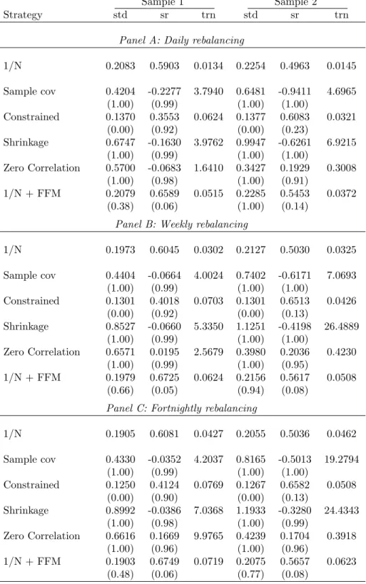
In Tables 2 and 3 we report the performance of several benchmark strategies, all of which do not use data on option prices. Table 2 gives the performance of minimum-variance
portfolios, and Table 3 gives the performance of mean-variance portfolios; both tables also report the performance of the 1/N portfolio. In Panel A of each table, we report the results for daily rebalancing, in Panel B for weekly rebalancing, and in Panel C for the case in which the portfolio is held for two weeks. We report three performance metrics in the table: the volatility (std) of portfolio returns, the Sharpe ratio (sr), and the turnover
(trn) of the portfolio. The p-value for the comparison with the 1/N benchmark is reported in parenthesis under each performance metric. Two p-values are reported in parenthesis under each performance metric: the first p-value is relative to the 1/N benchmark, and the second p-value in this table is relative to the “Sample-cov” benchmark. The p-value is for the one-sided null hypothesis that the portfolio being evaluated is no better than the 1/N benchmark for a given performance metric (so a small p-value suggests rejecting
the null hypothesis that the portfolio being evaluated is no better than the benchmark). Table 2 reports the performance of four variants of the minimum-variance benchmark portfolio: “Sample cov,” “Constrained,” “Shrinkage,” and “Zero correlation”. We see from this table that, compared to the 1/N portfolio, all of the strategies based on the minimum-variance portfolio achieve significantly lower volatility (bσ) out of sample. For example, in Panel A with results for “Daily rebalancing,” we see that for Sample 2, the volatility of the 1/N portfolio is 0.2254 and that of the minimum-variance portfolio based on the sample-covariance matrix with daily rebalancing is 0.1429, for the minimum-variance portfolio with shortsale constraints it is 0.1383, and for the minimum-minimum-variance portfolio with shrinkage it is 0.1263, and for the portfolio obtained from setting all cor-relations equal to zero it is 0.1899. The p-values indicate that the volatilities of the minimum-variance portfolios are significantly lower than that of 1/N. The results are similar for Sample 1 and in Panels B and C for “Weekly rebalancing” and “Fortnightly rebalancing.”
However, the Sharpe ratio (sr) and turnover (trn) are typically better for the 1/N portfolio compared to the four minimum-variance portfolios, with the only exceptions being the Sharpe ratio for the constrained minimum-variance portfolio, and for the minimum-variance portfolio obtained by setting all correlations equal to zero, in the case of Sample 2; but, for both cases the differences are not statistically significant.19
Of the four minimum-variance portfolios that we consider, the shortsale-constrained portfolio and the portfolio obtained by setting all correlations equal to zero have a
19It might seem strange to evaluate the Sharpe ratio of minimum-variance portfolios, whose objective is to only minimize the volatility of the portfolio. This comparison is motivated by the statement in Jagannathan and Ma (2003, p. 1653) that “the global minimum variance portfolio has as large an out-of-sample Sharpe ratio as other efficient portfolios when past historical average returns are used as proxies for expected returns.” DeMiguel, Garlappi, and Uppal (2009) also find that the minimum-variance portfolio performs surprisingly well in terms of Sharpe ratio when compared to other portfolios that rely on estimates of expected returns.
turnover that is comparable to that of the 1/N portfolio and substantially lower than the turnover of the unconstrained “Sample Cov” portfolio. This is true also in the tables that follow, where we use option-implied information.
Table 3 reports the performance of four mean-variance portfolios, “Sample cov,” “Constrained,” “Shrinkage,” and “Zero correlation,” and the mean-variance portfolio implemented using the parametric-portfolio methodology with the Fama and French characteristics along with momentum, which in the table is labeled “1/N + FFM.” The three mean-variance portfolios that do not have constraints on shortselling (“Sample cov,” “Shrinkage,” and “Zero correlation”) perform very poorly along all metrics. The mean-variance strategy with shortsale constraints achieves a lower volatility than the 1/N portfolio, but has a lower Sharpe ratio and higher turnover than the 1/N portfolio and also the shortsale-constrained minimum-variance portfolio considered in Table 2. The parametric portfolio usually has the best Sharpe ratio compared to the 1/N portfolio and the other mean-variance portfolios (though the difference is not always statistically significant), with a turnover that is comparable to that of 1/N. The volatility of the parametric-portfolio is higher than that of the shortsale-constrained mean-variance port-folio and the minimum-variance portport-folios considered in Table 2, which is not surprising given that this portfolio is not designed with the objective of minimizing volatility.
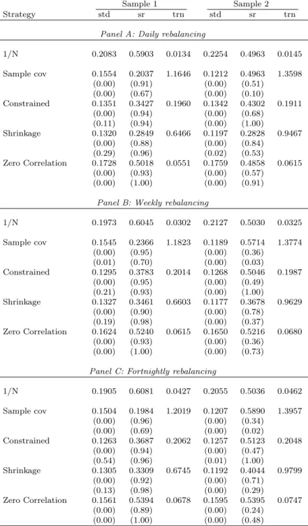
5.2
Performance of Portfolios Using Option-Implied Volatility
Motivated by the findings in Section 3.1 about the predictive power of model-free implied volatilities after correction for the risk premium,RV, we use them in diag(ˆc σ) to obtain thecovariance matrix given in (9); that is, ˆΣ = diag(RV) ˆc Ω diag(RV). Using this covariancec
matrix, and setting the expected return on each asset equal to the grand mean across all stocks, we determine the minimum-variance portfolio in Equation (8), along with the portfolios where shortsales are constrained, where shrinkage is applied to this covariance matrix, and where we impose the restriction that all correlations are equal to zero. In computing these portfolios, we continue to use historical correlations (except for the last portfolio, where correlations are set equal to zero).
The results for the minimum-variance portfolios based on risk-premium corrected option-implied volatility are given in Table 4. In this table we report two sets of p-values: the first with respect to the 1/N portfolio, and the second with respect to the corresponding benchmark portfolio in Table 2. For Sample 2, comparing the volatility (std) of portfolio returns across the different portfolio strategies, we see that the “Shrink-age” portfolio always achieves the lowest volatility, and this is significantly lower than that of the 1/N portfolio and also the “Shrinkage” benchmark strategy in Table 2, which uses historical volatility; however, the “Shrinkage” strategy has the lowest Sharpe ratio of all the strategies in Table 4, and also its turnover is quite high. For Sample 1, again the lowest volatility is achieved by the “Shrinkage” strategy, but for weekly and fortnightly rebalancing, it is the constrained strategy that has the lowest volatility. For both samples and all three rebalancing frequencies, of the four minimum-variance portfolios, it is the “Zero Correlation” portfolio that achieves the lowest turnover and the highest Sharpe ratio; for Sample 2, this Sharpe ratio is higher than even that of the 1/N portfolio.20
We conclude that volatility of stock returns estimated from risk-premium-corrected implied volatility is successful in achieving a significant reduction in portfolio volatility.21
5.3
Performance of Portfolios With Option-Implied Correlation
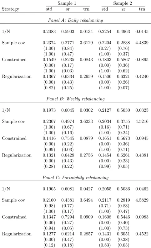
In this section, we investigate the gains from using option-implied correlations in portfolio selection. The performance of portfolios obtained from using the risk-premium-corrected option-implied correlations in (9), instead of historical correlations, is reported in Table 5. In order to isolate the effect of using implied correlations, we use volatilities calculated from historical data when computing the portfolio weights.We consider three minimum-variance portfolios in Table 5: the first is based on the sample-covariance matrix with option-implied correlations; the second, is the same as the first, but with shortsales constrained; and, the third, which is labeled “regularization,” replaces the “shrinkage” portfolio considered in the earlier tables. We use the
regulariza-20The reason for the relatively poor Sharpe ratio and turnover of the other portfolios based on implied volatility is that implied volatility is highly variable over time, which increases the variability of portfolio weights and reduces the gains from having a better predictor of realized volatility.
21For the portfolio constructed using implied volatilitywithout correcting for the risk premium, the volatility, Sharpe ratio, and turnover are worse than for the case where one uses the risk-premium-corrected implied volatility.
tion approach of Zumbach (2009) because we are using option-implied correlations, and hence, do not know the distribution of returns for the resulting covariance matrix, which means that we cannot use the shrinkage results of Ledoit and Wolf (2004a,b) that rely on particular distributional assumptions.
We observe from Table 5 that using the implied correlations does not lead to much of an improvement in the out-of-sample performance of the minimum-variance portfolios.22
While the volatility of the portfolios with shortsale constraints and regularization is less than that of the 1/N for both Sample 1 and Sample 2, it exceeds that of the correspond-ing benchmark portfolios studied in Table 2. The portfolios based on option-implied correlations also have higher turnover. The only positive result is that the Sharpe ra-tio of the constrained portfolio is greater than that of the 1/N portfolio and also the corresponding benchmark portfolio in Table 2, though the improvement is not always statistically significant.
Thus, we conclude that using the option-implied correlations does not lead to a sig-nificant improvement in portfolio performance. that the implied correlations almost fully eliminate the mean prediction error with respect to realized correlations. The reason for the poor performance of portfolios based on implied correlations is that the covari-ance matrix based on these correlations is highly unstable over time. Consequently, the resulting portfolio weights are highly variable and perform poorly out of sample.
5.4
Performance of Portfolios with Returns Predicted Using
Options
In this section, we examine the effect on portfolio performance of using four option-implied quantities that help forecast returns: the model-free option-implied volatility (MFIV); the volatility risk premium, measured as the spread between the currently observed Black-Scholes option-implied volatility and realized (historical) volatility (IRVS); model-free option-implied skewness (MFIS); and, skewness measured as the spread between the Black-Scholes implied volatilities for calls and for puts (CPVS). There are two ways in which we use these quantities to improve the performance of portfolios. In the first,
22The performance of portfolios based on implied correlations without the correction for the risk premium is slightly worse.
described in Section 4.3.1, we adjust the returns of the top and bottom decile portfolios based on each of these characteristics. In the second, described in Section 4.3.2, we use the parametric-portfolio methodology of Brandt, Santa-Clara, and Valkanov (2009).
5.4.1 Performance of Mean-Variance Portfolio With Option Characteristics
The out-of-sample performance of the mean-variance portfolios that use option-implied characteristics to adjust returns is reported in Table 6. There are four portfolios, each with shortsale constraints, considered in this table corresponding to the following four option characteristics: MFIV, IRVS, MFIS, CPVS. We compare performance of these portfolios to two sets of benchmarks: the 1/N portfolio, and the constrained minimum-variance portfolio reported in Table 2, which do not rely on option prices.23
From Table 6, we see that other than MFIV, the portfolios whose returns are adjusted based on any of the other three characteristics have a significantly higher Sharpe ratio than the 1/N portfolio and the benchmark portfolios in Table 3. The difference in Sharpe ratios is largest for daily rebalancing, and declines as the rebalancing frequency decreases. For example, in the case of Sample 1, the Sharpe ratio for the 1/N portfolio is 0.5903, while for the portfolio using IRVS it is 0.9232, for the portfolio using MFIS it is 1.0092, and for the portfolio using CPVS it is 1.4291. However, the improvement in the Sharpe ratio is accompanied by an increase in turnover.
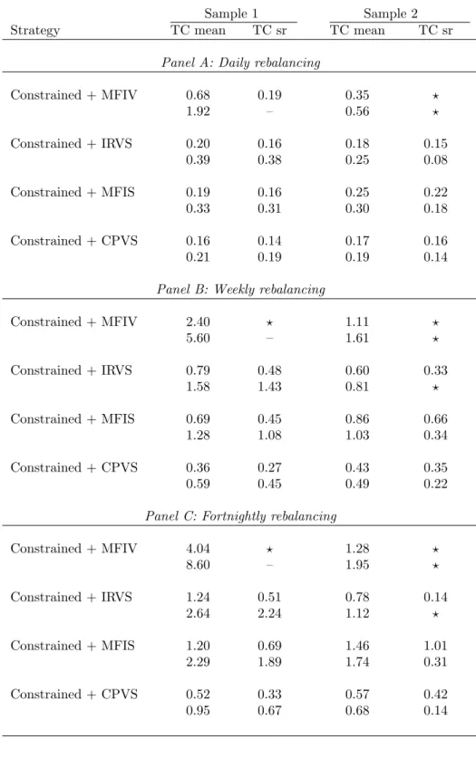
To understand if the mean-variance portfolios using option-implied characteristics to forecast expected returns outperform the benchmark portfolios even in the presence of transactions costs, we compute the equivalent transaction cost for each portfolio. Recall from Section 4.4 that this is the transaction cost level that equates the performance metric (mean return or Sharpe ratio) of a given strategy with that for the benchmark strategy.
In Table 7, for each dataset and rebalancing frequency, we report two sets of numbers, each set having two numbers. The first set of numbers are for the case where the bench-mark portfolio is the 1/N portfolio; the second set of numbers are for the case where the
23We use as a benchmark the shortsale-constrained minimum-variance portfolio rather than the con-strained mean-variance portfolios because the concon-strained minimum-variance portfolio has a better per-formance in terms of all three metrics.
benchmark is the constrained minimum-variance portfolio reported in Table 2. The first number in each set indicates the transaction cost that equates the mean return on the portfolio using option-implied characteristics to that of the benchmark portfolio. The second number is the transaction cost that equates theSharpe ratio of the two portfolios. For comparison, note that the typical cost for trading the stocks that are in our datasets is about 10 basis points (see French (2008)), with the actual cost depending on the size of the trade and the execution capability of the trader.
In Table 7, there are two possibilities when comparing the performance of portfolios that use option-implied information with the benchmark strategies. The first possibility is that the portfolio using option-implied information performs better than the benchmark portfolio, but has a higher turnover; in this case, the positive number reported in the table indicates the transaction cost the portfolio using option-implied information can incur before its performance drops to the level of the benchmark, which is also considered net of transactions costs. The second possibility is that the benchmark portfolio performs better, and has a better turnover. In this case there is no positive level of transaction costs that equates the two strategies, and we indicate this in the table with the symbol “?”. The third possibility is where the performance of both portfolios, net of transaction costs, turns negative; in the table we use “–” to represent this case.
We observe from Panel A of Table 7 that for the case of daily rebalancing, the equiva-lent transaction cost for the Sharpe ratio ranges from 14 to 56 basis points; for example, in the case of Sample 2, the portfolio with returns adjusted using MFIS has a higher Sharpe ratio than the 1/N portfolio for transactions costs of up to 22 basis points. In Panels B and C, we see that as the rebalancing frequency decreases, the equivalent trans-action cost increases; for example, in the case of Sample 2, the portfolio with returns adjusted using MFIS has a higher Sharpe ratio than the 1/N portfolio for transactions costs of up to 66 basis points for weekly rebalancing, and up to 101 basis points for fortnightly rebalancing.
We conclude from this analysis that information in MFIV, IRVS, MFIS, and CPVS can be used to improve the Sharpe ratio of mean-variance portfolios even after adjusting
for the higher transaction cost as a consequence of higher turnover in implementing the option-based strategy.
5.4.2 Performance of Parametric Portfolio Based on Option Characteristics
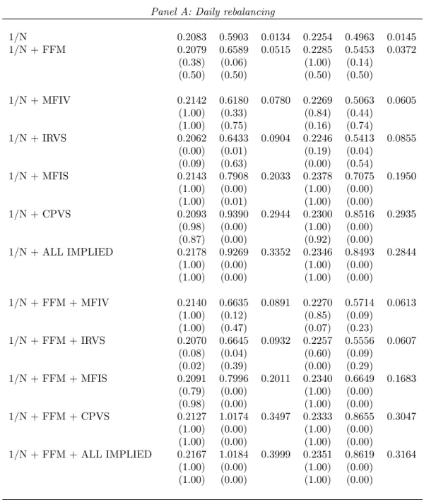
Next, we examine the out-of-sample performance of the parametric portfolios that use option-implied characteristics. We consider two benchmark portfolios: the 1/N portfolio and the mean-variance parametric portfolio “1/N + FFM” that starts with the 1/N portfolio and uses the FF and MOM characteristics to adjust the portfolio weights; we do not allow for shortsales. Comparing the two benchmarks, we see that the 1/N portfolio has a better turnover and volatility, but the parametric portfolio has a better Sharpe ratio.
From Table 8, we see that when we use the option-implied characteristics alone in-stead of the FFM, then the implied skewness measures (MFIS and CPVS) improve the risk-return tradeoff significantly compared to the two benchmarks. Moreover, the im-provement over 1/N is significant for daily, weekly and fortnightly holding periods, while the improvement over the parametric portfolio is significant only for daily rebalancing. For instance, in Panel A for Sample 1, the Sharpe ratio for the 1/N portfolio is 0.5903 and for the parametric portfolio with FFM factors it is 0.6589, while for the parametric portfolio with IRVS it is 0.6433, for the parametric portfolio with MFIS it is 0.7908, for the parametric portfolio with CPVS it is 0.9390; the results are similar for Sample 2. However, these gains are accompanied by higher turnover. Note that as the rebalancing period increases, the improvement decreases, while turnoverper rebalancing period stays at about the same level. This implies that the total transaction cost paid over the entire time period is decreasing.
We can also ask whether the option-implied characteristics improve performance if one is already using size, value, and momentum characteristics when selecting the para-metric portfolio. This question is answered in the second part of each panel of Table 8, where we consider each option-implied characteristic in addition to the FFM character-istics considered in the benchmark portfolio. From the lower part of each panel, we see that MFIS and CPVS improve the Sharpe ratio beyond the gains obtained from using
only the FFM characteristics. This improvement in Sharpe ratio for daily rebalancing is statistically significant for both Sample 1 and Sample 2 when using MFIS and CPVS; for weekly rebalancing it is statistically significant for CPVS for both samples, and for MFIS only for Sample 1; and, is not statistically significant for fortnightly rebalancing. Finally, looking at the last row of each panel where we add all four option-implied charac-teristics to the portfolio that already considers the FFM characcharac-teristics, we observe that the Sharpe ratio increases substantially and this improvement is statistically significant for daily and weekly rebalancing for both samples, and for fortnightly rebalancing it is significant for Sample 1.
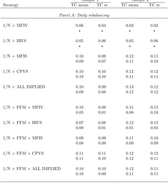
To understand if the portfolios using option-implied characteristics to forecast ex-pected returns outperform the benchmark portfolios even in the presence of transactions costs, just as before, we compute the equivalent transaction cost for each portfolio. In Table 9, for each dataset and rebalancing frequency, we report two sets of numbers, each set having two numbers. The first set of numbers are for the case where the bench-mark portfolio is the 1/N portfolio; the second set of numbers are for the case where the benchmark is the parametric portfolio with the FFM characteristics.
We observe from Panel A of Table 9 that for the case of daily rebalancing the benefits of using option-implied information would be eliminated if one had to pay a transaction cost of more than 11 basis points. This is because of the relatively higher turnover of the strategies using option-implied information. However, when we rebalance less frequently, then the benefits of using option-implied information survive higher transaction costs. For example, the results in Panel C of Table 9 for fortnightly rebalancing indicate that MFIS improves performance relative to the 1/N strategy even when we pay transaction costs of about 30 basis points. However, option-implied characteristics improve performance relative to the benchmark parametric portfolio for transaction costs of up to 10 basis points. Using all of the implied characteristics is beneficial in the presence of transaction costs of about 20 basis points with respect to the 1/N benchmark, and about 10 basis points for the parametric portfolio benchmark.
In summary, Table 9 suggests that in the presence of transactions costs, MFIS and CPVS are useful characteristics for choosing portfolios, while the value of using other
characteristics is smaller and their contribution is not robust across the two samples. Overall, the empirical evidence suggests that using option-implied skewness can lead to an improvement in the out-of-sample portfolio Sharpe ratio, even after adjusting for the higher transactions costs incurred by these strategies.
6
Conclusion
Mean-variance portfolio weights depend on estimates of volatilities, correlations, and expected returns of stocks. In this paper, we have studied how information implied in prices of stock options can be used to improve estimates of these three moments in order to improve the out-of-sample performance of portfolios with a large number of stocks. Performance is measured in terms of portfolio volatility, Sharpe ratio, and turnover. The benchmark portfolios are the 1/N portfolio; four types of minimum-variance portfolios and four types of mean-minimum-variance portfolios based on historical returns; and, the parametric portfolios of Brandt, Santa-Clara, and Valkanov (2009), based on historical returns and size, value, and momentum characteristics.
We find that using option-implied volatilities can lead to a significant improvement in portfolio volatility; however, option-implied correlations are less useful in reducing port-folio volatility. We also find that forming portport-folios using expected returns that exploit information in option-implied model-free skewness and implied volatility achieve a higher Sharpe ratio than portfolios that ignore option-implied information; this improvement in performance is present even after adjusting for transactions costs. Based on our empirical analysis, we conclude that prices of stock options contain information that can be useful for improving the out-of-sample performance of portfolios.
Table 1: Return Predictability
In this table, we report the results of various stock characteristics: size (SIZE), book-to-market (BTM), momentum (MOM), model-free implied volatility (MFIV), model-free implied skewness (MFIS), call-put-volatility spread (CPVS), and implied-realized-call-put-volatility spread (IRVS) to explain the cross section of returns. For each sample, on a daily basis, we sort the stocks by a particular characteristic, form the long-short decile portfolio, and hold this period for a particular holding period (one week, two weeks, or one month). Below, we show the annualized mean holding return for each decile-based portfolio and in the parenthesis the p-value for the hypothesis that the mean return is not different from zero. The p-values are based on the Newey and West (1987) autocorrelation-adjusted standard errors with the lag equal to the number of overlapping periods in portfolio holding.
Sample 1 Sample 2
Characteristic 1 day 1 week 2 weeks 1 day 1 week 2 weeks
SIZE -0.1705 -0.1729 -0.1623 -0.1543 -0.1543 -0.1511 (0.00) (0.00) (0.00) (0.00) (0.00) (0.00) BTM 0.2050 0.1983 0.1853 0.1463 0.1365 0.1337 (0.00) (0.00) (0.00) (0.00) (0.00) (0.00) MOM 0.0026 -0.0148 -0.0325 -0.0034 -0.0060 -0.0160 (0.49) (0.42) (0.34) (0.48) (0.46) (0.41) MFIV 0.3055 0.2674 0.2243 0.1694 0.1497 0.1174 (0.00) (0.00) (0.00) (0.07) (0.06) (0.09) IRVS 0.1477 0.0959 0.0610 0.1535 0.0911 0.0479 (0.01) (0.01) (0.06) (0.01) (0.01) (0.09) MFIS 0.3721 0.1651 0.1465 0.4640 0.2337 0.1798 (0.00) (0.00) (0.00) (0.00) (0.00) (0.00) CPVS 0.7581 0.1899 0.1061 0.8699 0.2477 0.1421 (0.00) (0.00) (0.00) (0.00) (0.00) (0.00)