ABSTRACT
This study investigates taxi drivers’ multi-day cruising behaviours with GPS data collected in Shenzhen, China. By calculating the inter-daily variability of taxi drivers’ cruising behaviours, the multi-day cruising patterns are investigated. The impacts of learning feature and habitual feature on multi-day cruising behaviours are determined. The results prove that there is variability among taxis’ day-to-day cruising be-haviours, and the day-of-week pattern is that taxi drivers tend to cruise a larger area on Friday, and a rather focused area on Monday. The findings also indicate that the impacts of learn-ing feature and habitual feature are more obvious between weekend days than among weekdays. Moreover, learning fea-ture between two sequent weeks is found to be greater than that within one week, while the habitual feature shows reces-sion over time. By revealing taxis' day-to-day cruising pattern and the factors influencing it, the study results provide us with crucial information in predicting taxis' multi-day cruising locations, which can be applied to simulate taxis' multi-day cruising behaviour as well as to determine the traffic volume derived from taxis' cruising behaviour. This can help us in planning of transportation facilities, such as stop stations or parking lots for taxis. Moreover, the findings can be also em-ployed in predicting taxis' adjustments of multi-day cruising locations under the impact of traffic management strategies. KEY WORDS
taxi; multi-day; cruising pattern; GPS;
1. INTRODUCTION
Taxi is one of the major transportation modes in urban transportation system. Yet, empty taxi cruising results in significant amount of wasted energy and emissions. As we know, up to 40 percent of taxis’ daily mileage is spent with no passengers on board [1]. The average dead mileage for taxis in Beijing is 120 km per day, which accounts for 40% of total daily mileage. This means that 13 litres of fuel are used per day while driving with no passengers [2]. Therefore, it is import-ant to identify ways to make empty taxis cruise more efficiently. This paper aims at learning taxis’ multi-day cruising patterns and providing important information for taxi drivers and transportation managers to en-hance taxis’ cruising efficiency. By investigating the factors that affect taxi drivers’ cruising decisions and by examining their multi-day cruising behaviours, we will try to find the underlying mechanisms of taxis’ day-to-day cruising decisions.
In recent years, massive progress has been made in travel survey with the rapid development and appli-cation of Global Positioning System (GPS) technolo-gy. As an advanced computer-based technique, GPS offers significant advantages over traditional survey methods in collecting travel data, especially its ability to capture multi-day data [3]. Many researchers
pre-UNDERSTANDING TAXI DRIVERS’ MULTI-DAY
CRUISING PATTERNS
FANG ZONG, Ph.D.
E-mail: zongfang@jlu.edu.cn
Jilin University, College of Transportation
5988 Renmin Street, Changchun, Jilin, 130022, China XIAO SUN, Prof.
Corresponding author E-mail: sunxiao@jlu.edu.cn
Jilin University, Applied Technology College
5372 Nanhu Road, Changchun, Jilin, 130022, China HUIYONG ZHANG, Ph.D.
E-mail: 15143173332@163.com Jilin University, School of Management
5988 Renmin Street, Changchun, Jilin, 130022, China XIUMEI ZHU, Ph.D.
E-mail: xmzhu@jlu.edu.cn, 327514076@qq.com Jilin University, School of Management
5988 Renmin Street, Changchun, Jilin, 130022, China WENTIAN QI, M.S.
E-mail: 492953906@qq.com
Suzhou Institute of Construction and Communications Suzhou, Jiangsu, 215000, China
Traffic Management Original Scientific Paper Submitted: Sep. 25, 2014 Approved: Nov. 24, 2015
sented studies on taxi’s driving behaviours by using GPS data [4]. This study will use multi-day GPS data collected from 2,536 taxi drivers in Shenzhen, China. As GPS-collected data are not ready for direct use in cruising behaviour analysis, some computer-based techniques and methods will be used, such as Quad-rat Analysis and Entropy, in processing and analysing GPS data.
With wide application of GPS devices in multi-day travel survey, the analysis of multi-day travel behaviour has been one of the hot issues in transportation stud-ies. However, none of the researchers analysed the multi-day operating patterns or modelled the process of day-to-day dynamics of taxis’ cruising behaviours. In this paper an analysis of taxis’ multi-day cruising pat-terns will be conducted. Two major features of taxis’ day-to-day cruising behaviours, i.e., learning from pre-vious pick-up experience (learning feature) vs. obeying cruising habits (habitual feature), will be investigated. In particular, we seek to answer three questions: 1) Is there variability between taxi drivers’ day-to-day cruis-ing behaviours? 2) What are the differences among multi-day cruising behaviours? 3) How do the two fac-tors, i.e., learning and habits, affect taxi drivers’ day-to-day cruising behaviours?
The remainder of this paper is organized as follows. Section 2 presents a review on the analysis of taxis’ cruising behaviours in general. Section 3 presents a description of data and the study area. In Section 4 the spatial distributions of cruising traces and pick-up points are examined. In Section 5, the multi-day variability of cruising patterns is calculated, and the different impacts of learning feature and habitual fea-ture in day-to-day cruising behaviours are investigated. The paper is concluded with Section 6, in which the findings are summarized and the directions for future research discussed.
2. LITERATURE REVIEW
The multi-day travel behaviour analysis has been one of the hot issues in transportation research. How-ever, none of the studies analysed the multi-day op-erating pattern or modelled the day-to-day dynamics of taxis’ cruising behaviours. There’re only a few re-searchers who considered previous operating experi-ence in modelling taxis’ driving patterns. For example, Reference [5] modelled a taxi service system in urban areas, taking into account the taxi drivers’ knowledge of the transportation network from their day-to-day experience. Reference [6] found that driver’s travel experience as well as a renewal of all acquirable traf-fic information that can assist in confirming the ref-erence points in road network have influence on the route choice of the next trip. Reference [7] presented an experiential approach to compute optimal paths, in which path-planning was supported by a flexible road
network hierarchy using the experience of taxi drivers. Other studies that investigated driving experience are Yu et al.’s work on modelling bus arrival times [8, 9] and vehicle’s route choice [10], and Yao et al.’s study on accident detection [11], etc.
Several models were developed to investigate the day-to-day dynamics of travel behaviours, such as ref-erence [12] proposed a stochastic process approach to analyse day-to-day dynamics in a transportation network. A key assumption of the stochastic process is that the path choice probabilities are time homo-geneous, which means that there are no time-depen-dent variations in drivers' perceptions. This approach was further extended by reference [13] to include day dynamics. Reference [14] described a simple route choice model over time whereby decisions are based on the weighted average of previous travel decisions’ utilities. Based on this model, reference [15] proposed a myopic adjustment model by allowing the weights to vary across individuals. Reference [16] presented detailed discussions regarding the habitual and vari-able behaviour of individuals over time. They noted that some behaviours, when examined in a disjointed framework (say, a work trip examined in isolation of the overall daily activity-travel pattern), are repeated on a day-to-day or week-to-week basis. However, when the overall daily activity-travel pattern is examined in its entirety, they found that a one-day pattern is not representative of a person’s routine travel.
Previous studies also proposed two major features of multi-day travel decisions: learning feature vs. ha-bitual feature. With respect to learning feature, some researchers mentioned above proved that taxi drivers have the characteristics of learning, which means that they will update their traffic information from their day-to-day experience and use the information in route choice of the next trip [5, 6]. Besides taxi relat-ed studies there are also some researchers who mod-elled the learning process of other travel behaviours. For example, reference [17] proposed travellers’ deci-sion-making process based on Bayesian updating by considering day-to-day dynamics of travel behaviours. Reference [14] proposed a learning model for route choice selection. Reference [18] developed a learning model for mode choice.
The habitual feature has been also proved and uti-lized by many studies related to travel behaviour anal-ysis. In many studies about mode choice modelling, the factor of habit was also taken as a major variable [19, 20]. Reference [21] demonstrated that when be-haviours are well-practiced and repeatedly performed, frequency of past behaviour reflects habit strength and has direct effect on future performance. Reference [22] found that although most drivers thought that they had two or three alternative routes, the majority said they always stuck to the same one. This also demon-strated the crucial role of habits in travel decisions.
Though the above studies proved that travel be-haviours have the learning features and habitual features, none of them conducted a quantitative comparison between them. This study will present a quantitative comparison between these two features, and measure the multi-day variability of taxi drivers’ cruising patterns.
3. DATA AND STUDY AREA
The data used in this study are GPS traces collect-ed from 2,536 taxis during a 9-day period (November 18th 2011 – November 26th 2011), in Shenzhen, China.
The surveyed taxis account for about 17.14% of the to-tal number of taxis and 76.64% of taxis with on-board GPS equipment in Shenzhen. Each record in the data-set represents a GPS signal that was captured con-secutively at a 5-second interval (Shenzhen Transport Information Center, 2011). The basic information pro-vided by the dataset contain taxis’ traces in longitude and latitude form, vehicle identification, operation sta-tus (empty or occupied), timestamp, spot speed, and azimuth. During the 9-day period, 30,179,212 valid positions in total were recorded.
In order to learn the multi-day cruising patterns as well as the features of cruising behaviours, two types of points are selected from the GPS traces, i.e., cruising traces (without passengers) and pick-up points (loca-tions whose operation status is from vacancy to occu-pancy), in which cruising traces represent taxi drivers’ cruising patterns. The spatial correlations among different days’ cruising traces and pick-up points are used to represent learning vs. habitual features.
The study area of this paper is the urban area of Shenzhen city, which is one of the four most developed cities in China. It had a residing population of 10.63 million in 2013 and 10 districts. The administrative di-vision of Shenzhen is shown in Figure 1.
As GPS-collected data are not ready for direct use in cruising behaviour analysis, one of the widely used spatial analysis techniques – Quadrat Analysis – will be employed in data processing. According to the theo-ry of Quadrat Analysis, the entire study area is divided into cells. The area of each cell (Areag) can be
calcu-lated as:
Areag= 2A/Q (1),
where A is the entire study area and Q is the number of traces that will be analysed in the study area. The X and Y coordinates for the study area range from 167.53 to 255.81 and from 2,486.22 to 2,531.10, respectively. Based on these ranges, the total area A can be calcu-lated as 3,962.20 square kilometres. Since this study is concerned with drivers’ traces on one day, the aver-age number of GPS traces of each driver per day, i.e., 9,083, is taken as the value of Q. Thus, the area of each cell is then calculated as 0.8724 square kilome-tres, with each side being equal to 0.9340 km. Thus, the study area is divided into 96×50=4,800 cells. For X coordinate, there are (255.81-167.53)/0.93=94.92 segments, and for Y coordinate, there are (2,531.10-2,486.22)/0.93=48.26 segments. In order to cover the four sides of the study area as well as to make the numbers of the segments integers, one cell is ex-panded for each side of the study area. This yields 96 and 50 segments for X coordinate and Y coordinate, respectively.
CBD
4. SPATIAL DISTRIBUTIONS OF CRUISING
TRACES AND PICK-UP POINTS
4.1 Entropy
By employing a parameter of entropy, which is a measure of the uncertainty in a random variable [23], the basic characteristics of spatial distribution of cruis-ing traces and pick-up points can be examined. If we define a discrete random variable Z as the event that one point locates in a zone, then the entropy of Z, i.e.
H(Z), refers to the unpredictability of event Z: 25 1 ( ) iln( )i i n n H Z N N = = -
∑
(2)in which, ni is the number of points in zone i with i = 1,
2, …, 25 (the study area is divided into 25 zones as shown in Figure 1), N is the total number of points, that is 25 1 i i N n = =
∑
, then niN means the probability that one point is located in zone i, and 25
1 1 i i n N = =
∑
.When all the points are located in one zone, we can get the minimum value of H(Z), that is 0, which means that event Z is most predictable, or points are most clustered concerning spatial distribution. On the con-trary, when all the points are located in 25 zones even-ly, we can get the maximum value of entropy, defined as Hm, which means that event Z is most
unpredict-able, or points are most dispersed concerning spatial distribution. In this study, Hm= ln 25, which is obtained
from probability 1
25
i n
N = for each zone i. Then C can be introduced to represent the cluster degree of points:
C= 1 -H(Z)/Hm (3)
As we know, C is a value between 0 and 1. The higher the cluster degree C is, the more clustered the spatial distribution of points is. According to reference [24]' study, cluster degree>0.45 means that the data points are very clustered, and 0.4 <C≤ 0.45 denotes that the data points are clustered, while C≤ 0.4 means that the points are dispersed.
4.2 Analysing spatial distribution with entropy The mean value of cluster degree C of cruising trac-es and pick-up points per person per day is calculated to be 0.6080 and 0.6936, respectively. This indicates that both cruising traces and pick-up points exhibit a very clustered spatial distribution. As the cluster de-gree C of pick-up points is bigger than that of cruis-ing traces, we can infer that pick-up points are more clustered than cruising traces in spatial distribution. One potential reason is that the taxis’ pick-up points are also the start points of taxi trips, and the spatial
distribution of the start points is related to the spatial distribution of land use and population in the study area [25]. In the study area of this paper, i.e., Shen-zhen city, the high-density area of land use and popu-lation is the area covered by Luohu and Futian district (shown in Figure 1). It is the clustered spatial distribu-tion of land use and populadistribu-tion that leads to the aggre-gated spatial distribution of taxis’ pick-up points. On the contrary, the spatial distribution of cruising traces depends on taxi driver’s individual cruising behaviour, which is much more a subjective factor, comparing with land use and population distribution which are objective factors. Being the results of subjective de-cision behaviours, cruising traces are then more dis-aggregated than pick-up points in spatial distribution. 4.3 Variability in multi-day cluster degrees
In order to identify the potential variability in multi-day cruising patterns, we will measure the changes among multi-day cluster degrees of cruising traces, and compare them with those of the pick-up points. As the GPS traces recorded the cruising traces of dif-ferent days and difdif-ferent taxis, the total variability in GPS records contain both inter-daily variability and in-ter-personal variability. Therefore, in order to identify the variability among multi-day cruising behaviours, a distinction should be made between inter-daily vari-ability and inter-personal varivari-ability. Reference [26] and [27] provided the theory of TSS (total sum of squares) to measure and quantify the inter-personal variability and intra-personal variability in a travel sur-vey data set. Figure 2 shows the framework of TSS as adopted from their work.
Inter-personal variability refers to the differences in the behaviour among different individuals on the same days. Behavioural differences among taxi drivers may be explained partially by differences in the istics of individuals. By incorporating such character-istics into a model, one can account for systematic differences in behaviour among individuals. The por-tion of inter-personal variability that can be explained systematically through differences in socio-economic characteristics is referred to as explained variability. The remainder is referred to as unexplained variability. Similarly, intra-personal variability (inter-daily vari-ability) may also be considered as having two com-ponents. The first component is called systematic day-of-week variability. This refers to the portion of intra-personal variability that may be attributed to sys-tematic day-of-week effects. Intra-personal variability that cannot be explained by day-of-week effects is random and is referred to as residual intra-personal variability.
In this study, the total intra-personal (inter-daily) variability as well as the total inter-personal variability will be quantified by employing the TSS theory. The
to-tal variability in various measures of cruising patterns is split into two components which are represented by appropriate sums of squares. In this representation, the total variability is represented by the total sum of squares (TSS), as follows:
2 ( ij ) i j
TSS=
∑∑
C C- (4)where Cij is the cluster degree C of person i on day j,
and C is defined as the overall sample mean of C per person per day.
The inter-personal sum of squares (IPSS) is given by: 2
( )
i i i
IPSS=
∑
J C C- (5)where Ji is the number of days for which individual i
reported GPS cruising trajectory, and Ci means the cluster degree C of person i per day.
The inter-daily sum of squares (IDSS) is given by: 2 ( ij i) i j IDSS=
∑∑
C C- (6) Also, we have: ij j i i C C J =∑
(7) and ij i i i j i i i i i C J C C J J =∑
=∑∑
∑
∑
(8)It can be readily seen that,
TSS=IPSS+IDSS (9)
Therefore, the ratio IDSS/TSS provides a measure of the proportion of total variability in cruising patterns that may be attributed to inter-daily variability. Simi-larly, IPSS/TSS provides a measure of the proportion of total variability in cruising patterns that may be at-tributed to inter-personal variability.
The calculating results of TSS parameters for clus-ter degrees of cruising points and pick-up points are shown in Table 1. The results indicate that, for both cruising traces and pick-up points, the value of IPSS
is greater than that of IDSS: the inter-personal variabil-ity and inter-daily variabilvariabil-ity can explain 66.27% and 33.73% of the total variability in cluster degree of the cruising traces, respectively; Similarly, the inter-per-sonal variability and inter-daily variability can explain 64.53% and 35.47% of the total variability in cluster degree of the pick-up points, respectively. Concerning the results of cruising traces, because IPSS accounts for 66.27% of the total variability it indicates that there is large variability between different taxi drivers. In other words, different types of taxi drivers may have different strategies for cruising location choice: some of them may cruise in a large area, while some of them may choose a relatively small area.
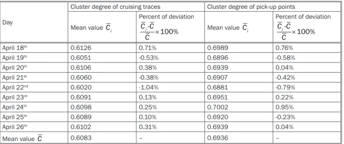
In order to explain the inter-daily variability in cruis-ing traces and pick-up points, the mean values of clus-ter degree of different days per person are calculated. The results are shown in Table 2.
Total Variability Intra-personal Variability Residual Intra-personal Variability Systematic, Day-of-week Variability Unexplained Variability Explained Variability Inter-personal Variability
Figure 2 – Methodological framework for measuring inter-personal/intra-personal variability
Table 1 – TSS parameters for cluster degrees
Item Cluster degree of cruising traces Cluster degree of pick-up points
Value Ratio Value Ratio
TSS 73.81 – 52.65 –
IPSS 48.91 IPSS/TSS: 66.27% 33.98 IPSS/TSS :64.53%
The results indicate that there are two similar char-acteristics for the multi-day variability of both cruis-ing traces and pick-up points’ cluster degree: (1) the multi-day variability is small, i.e., the cluster degrees of different days are similar to each other; (2) there is a same day-to-day changing pattern, i.e., the cluster de-gree reaches the minimum on April 22nd (Friday). One
of the reasons may be that on Friday passengers made taxi trips not only for the working purpose like other weekdays, but also for other trip purposes, such as en-tertainment and maintenance, like on weekend. This relative complicated composition of trip purposes on Friday leads to the disaggregated distribution of both cruising traces and pick-up points.
Concerning the maximum of cluster degree, the val-ue on April 18th (Monday) is the maximal value in the
multi-day cluster degrees of cruising traces. A potential reason is that most of the taxi trips on Monday are working trips, and taxi drivers may choose a "Monday cruising mode" according to their own cruising habits or land use characteristics of the city. It may be the relatively regular "Monday cruising mode" that makes the distribution of cruising traces more clustered than other days of the week. As for the pick-up points, the maximum of cluster degree is the value on April 24th
(Sunday). A potential reason is that most of the taxi trips on Sunday are trips for entertainment or main-tenance purposes starting from a high-density area, such as the Central Business District. Therefore, the pick-up points concentrate on the high-density areas and present an aggregated distribution.
5. LEARNING AND HABITUAL FEATURES
OF CRUISING BEHAVIOUR
The learning feature means that taxi drivers re-member their previous cruising experience, learn from it, infer potential pick-up locations from it, and apply
them in future cruising location choices. In this pa-per, the spatial correlation between current cruising traces and previous pick-up points tj&pj- is chosen to
represent the learning feature. The footmark j denotes current day and j- refers to previous day, t and p rep-resent cruising traces and pick-up points, respectively. Habits denote one’s customary ways of behaving [21, 28]. In this paper, the habitual feature presents that taxi drivers will accumulate some cruising hab-its from day-to-day cruising experience and follow the cruising habits consciously or unconsciously in future cruising decisions. The similarity in spatial distribution between current cruising traces and previous cruising traces (tj&pj-) is taken as the habitual feature in
cruis-ing pattern. A diagram of the learncruis-ing feature and ha-bitual feature is shown in Figure 3.
Current cruising traces Learning feature: tj & pj– Habitual feature: tj & tj– Previous cruising traces Previous pick-up points
Figure 3 – A diagram of learning feature and habitual feature Table 2 – Multi-day cluster degrees
Day
Cluster degree of cruising traces Cluster degree of pick-up points Mean value Cj Percent of deviation -100% j C C C × Mean value Cj Percent of deviation -100% j C C C × April 18th 0.6126 0.71% 0.6989 0.76% April 19th 0.6051 -0.53% 0.6896 -0.58% April 20th 0.6106 0.38% 0.6939 0.04% April 21st 0.6060 -0.38% 0.6907 -0.42% April 22nd 0.6020 -1.04% 0.6881 -0.79% April 23rd 0.6091 0.13% 0.6951 0.22% April 24th 0.6098 0.25% 0.7002 0.95% April 25th 0.6089 0.10% 0.6920 -0.23% April 26th 0.6102 0.31% 0.6939 0.04% Mean value C 0.6083 – 0.6936 –
As Figure 3 shows, the relationship between tjand pj-, such as the distance between current cruising
trace and previous pick-up point, is selected to repre-sent the learning feature of cruising behaviour. Simi-larly, the relationship between tjand tj- can be seen as
taxi driver’s habitual feature in cruising decision. 5.1 Analysing the distance between hot spots
One of the most direct approaches to measure spa-tial correlation between spaspa-tial points is to calculate the distance between them. To do this, we first identify the hot spots of cruising traces and pick-up points for each driver and each day, and then take the hot spots as representations of cruising traces and pick-up points, respectively, for distance calculation. Accord-ing to the theory of hot spot analysis, we calculate the number of cruising traces and pick-up points for each taxi and each day in each cell of the study area. The centroid of the cell with the largest amount of cruis-ing traces or pick-up points is noted as the hot spot of cruising traces or pick-up points, respectively. Then one taxi’s one day’s cruising traces and pick-up points can be represented by their calculated hot spot.
The distance between the hot spots of current cruising traces and previous pick-up points can be defined as D(tj, pj-), and the distance between the hot
spots of current cruising traces and previous cruising traces is noted as D(tj, tj-). The mean value of D(tj, pj-1)
and D(tj, tj-1) per driver is calculated as 6.94 km and
6.20 km, respectively. j-1 and j denote sequential two days in the 9-day period. This indicates that the dis-tance between today’s cruising traces and yesterday’s cruising traces is smaller than that between today’s cruising traces and yesterday’s pick-up points. This re-veals that, concerning the distance between hot spots,
habitual feature is a more important factor than learn-ing feature in taxi drivers’ cruislearn-ing location choice.
In order to measure multi-day variability of learn-ing feature and habitual feature, the theory of TSS
mentioned above is adopted. In equations (4) to (8), the cluster degree related parameters can then be switched to distance related parameters which pres-ent distances among hot spots of multi-day cruising traces and pick-up points. The results of TSS analysis for distance between hot spots are shown in Table 3.
The IDSS and IPSS value of D(tj, pj-1) reveals that
there are both inter-personal and inter-daily variabili-ties concerning taxi drivers’ learning feature. However, the inter-personal variability is a little bit greater than the inter-daily variability. This reveals that different types of taxi drivers have different cruising behaviours concerning the learning feature. In other words, dif-ferent taxi drivers are found to have difdif-ferent levels of ability to learn from previous pick-up experiences. Therefore, when measuring taxi drivers’ learning fea-ture, not only multi-day variability but also variability among different types of drivers should be considered.
The ratios IDSS/TSS and IPSS/TSS for D(tj, tj-1)
show that the inter-daily variability accounts for 63.27% of total variability and the inter-personal vari-ability covers 36.73% of total varivari-ability. This shows a larger variability of multi-day habitual feature than that of inter-personal habitual feature. In other words, it proves that a taxi driver has different cruising habits on different days of the week. The multi-day changes of cruising habits should be considered in cruising pat-terns analysis.
Therefore, further analysis of multi-day variability is conducted by calculating multi-day distance between
tj&tj-1 and tj&pj-1 hot spots. The results are shown in
Table 4.
Table 3 – TSS parameters for distances between hot spots
Item D(tj, pj-1) D(tj, tj-1)
Value Ratio Value Ratio
TSS 3,081,451 – 2,832,022 –
IPSS 1,586,149 IPSS/TSS: 51.47% 1,040,226 IPSS/TSS: 36.73%
IDSS 1,495,303 IDSS/TSS: 48.53% 1,791,797 IDSS/TSS: 63.27%
Table 4 – Statistics of distance between multi-day hot spots
Time D(tj, pj-1) D(tj, tj-1)
Value (km) Standard deviation Value (km) Standard deviation
Mean value per day 6.94 10.79 6.20 10.34
Day of week
Between two consecutive
weekdays 7.45 8.65 6.50 7.64
Sunday and Saturday 6.59 10.31 6.08 9.95
Saturday and Friday 6.92 10.80 6.40 10.72
Between days of two consecutive weeks
Between Mondays 6.95 10.97 6.95 10.97
The smaller the distance, the larger is the correla-tion between the two types of spatial points. Concern-ing habitual feature, the results show that, for two con-secutive days, the habitual feature between Sunday and Saturday is the largest, while that between two weekdays is the smallest. This indicates that the im-pacts of habits are more obvious between weekend days than among weekdays. The distances between
tj&tj-1 hot spots of two consecutive weeks reveal that
there are also cruising habits between two consecu-tive weeks. However, the impacts of cruising habits of two weeks is smaller than those within one week.
The results reveal a similar pattern of inter-daily learning feature in one week as the one of the habitu-al feature, that is, the learning degree between Sunday and Saturday is the largest among learning degrees between two consecutive days in one week, while that between two weekdays is the smallest. This indicates that the impacts of learning feature are more obvious between weekend days than among weekdays. In oth-er words, taxi drivoth-ers considoth-er more yestoth-erday’s pick-up experience on Sunday than on other days of the week. The distances between tj&pj-1 hot spots of two sequent
weeks reveal that taxi drivers also accumulate cruising knowledge from pick-up points of last week. Moreover, the learning degrees between two consecutive weeks are greater than those within one week. This reveals that learning feature does not decay over time as ha-bitual feature does.
5.2 Analysing frequency of the hot spots in the same cell
Besides distance between hot spots, the probabil-ity of tj&pj-1 hot spots vs. tj&tj-1 hot spots being in the
same cell is also adopted to measure multi-day learn-ing feature vs. habitual feature of cruislearn-ing behaviour, respectively. In detail, the probability that the hot spots of current cruising traces and previous pick-up points are in the same cell is defined as P(tj, pj-1), and is taken
as a parameter to measure the learning feature of the cruising behaviour. Similarly, the probability that the hot spots of current cruising traces and previous cruis-ing traces are in the same cell is defined as P(tj, tj-1)
in order to be adopted in examining habitual feature of cruising behaviour. P(tj, pj-) and P(tj, tj-) are given by:
1 -( , ) I tp i i j j P t p I d = =
∑
(10) where dtpi is an indicator parameter, dtpi= 1 if driver i’s
hot spots of cruising traces on day j (current) and pick-up points on day j- (previous) are in a same cell, and
dtp
i= 0 if their hot spots of cruising traces on day j and
pick-up points on day j- are not in the same cell. I is the total number of taxi drivers.
1 -( , ) I tt i i j j P t t I d = =
∑
(11) where dtti is another indicator parameter, dtti= 1 if
driv-er i’s hot spots of cruising traces on day j and cruising traces on day j- are in the same cell, and dtt
i = 0 if the
hot spots of cruising traces on day j and cruising traces on day j- are not in the same cell.
The results (shown in Table 5) indicate that 41.69% of the taxi drivers chose the same cruising area (hot spot) according to previous day’s cruising area, while only 13.75% of taxi drivers chose the same cruising area as previous day’s pick-up hot spot. This indicates that taxi drivers prefer to obey cruising habits more than to learn from previous pick-up knowledge. This finding is similar to the result obtained from the hot spot analysis presented above.
The results also show similar multi-day variability of learning feature and habitual feature: the impacts of learning feature and habitual feature between Sunday and Saturday is the largest among the values between two consecutive days in one week, respectively, while that between two weekdays is the smallest. Moreover, the difference between learning feature and habitual feature is that learning feature between two consecu-tive weeks is greater than that within one week, while the habitual feature presents recession over time.
6. CONCLUSION
This study investigates taxi drivers’ multi-day cruis-ing behaviours by uscruis-ing GPS data collected in Shen-zhen. Our results show that the inter-daily variability can account for 33.73% of the total variability in clus-ter degree of the cruising traces. This answers the
Table 5 – Probabilities of different hot spots being in the same cell
Time P(tj, pj-) P(tj, tj-)
Mean value per day 13.75 41.69
Day of week
Between two consecutive weekdays 13.34 40.44
Sunday and Saturday 14.29 43.55
Saturday and Friday 13.75 41.15
Between days of two consecutive weeks Between Mondays 13.30 36.11
first question that we proposed in Section 1: there is variability between taxi drivers’ day-to-day cruising be-haviours.
By investigating the TSS statistics of cluster de-grees of multi-day cruising traces, the second question proposed in Section 1 is answered. Our findings reveal that there are minor differences among cluster de-grees of multi-day cruising traces. The cluster degree reaches the minimum on April 22nd (Friday) and the
maximum on April 18th (Monday), which reveals that
taxi drivers tend to cruise a larger area on Friday but a focused area on Monday.
To answer question 3, we conducted a comparison of the impacts of learning and habitual feature on day-to-day cruising traces. The results show that different types of taxi drivers obey the previous pick-up expe-rience in different degrees. At the same time, a taxi driver has different degrees of cruising habits on dif-ferent days of a week. This suggested that we should pay attention to the variability among different types of drivers concerning learning feature, while considering the day-of-week characteristic for the habitual feature of cruising behaviours. The results also show similar multi-day variability of learning feature and habitual feature: the impacts of the two features are more ob-vious between weekend days than among weekdays. However, learning feature between two consecutive weeks is greater than that within one week, while the habitual feature presents recession over time.
By revealing taxis' day-to-day cruising pattern and the factors influencing it, the study results provide cru-cial information in predicting taxis' multi-day cruising locations. In detail, the probability can be calculated that a driver will choose a location as today's cruising location by considering their cruising locations and pick-up points in the previous days. This finding can be applied to simulate taxis' multi-day cruising behaviour. Moreover, when making a traffic management strate-gy, we can also employ the study results in predicting taxis' adjustments of multi-day cruising locations un-der the impact of the strategy. This work also makes a contribution in determining the traffic volume derived from taxis' cruising behaviour in the study area. This finding is essential for planning of transportation facili-ties, like stop stations or parking lots for taxis.
It should be pointed out that only learning feature and habitual feature are considered in this paper. In reality, there may be other factors, such as last drop-off location, land use characteristics [29] and traffic condition [28, 30, 31], that have potential effects on taxis’ cruising behaviour. Further study should be con-ducted to model the impacts of these factors. Besides, in order to get more information concerning multi-day cruising patterns, the GPS data of more days should be used in the future study.
ACKNOWLEDGEMENTS
The research is funded by the National Natural Sci-ence Foundation of China (50908099), the Humani-ty and Social Science Youth foundation of Ministry of Education (14YJC630225), the China Postdoctoral Science Special Foundation (2014M551191) and Jilin University outstanding youth fund (2013JQ007). Spe-cial thanks to the anonymous reviewers whose valu-able comments helped tremendously to improve this paper. 出租车的多日巡航行为研究 宗芳1,孙晓2,张慧永3,朱秀梅3,祁文田4 1吉林大学交通学院 长春 中国 2吉林大学应用技术学院 长春 中国 3吉林大学管理学院 长春 中国 4苏州建设交通高等职业技术学校 苏州 中国 本文应用深圳市的出租车车载GPS数据分析了出租车 的多日的空载巡航行为。通过计算出租车各日巡航点空间 分布特征值间的变化,分析总结了巡航行为的多日变化规 律。对比分析了司机的学习性和习惯性对巡航行为的影 响。研究结果表明出租车逐日的巡航行为间具有一定差 异:他们倾向于在周五巡航更大的区域范围,而周一的巡 航区域比较集中;另外,周六和周日之间学习性和习惯性 的影响较每周工作日之间的表现更明显;同时,两周之间 的学习性比一周内的影响更大,而习惯性的影响具有随时 间增长而衰减的特征。本文的研究成果体现了出租车的多 日巡航行为决策机理,对于提出有效措施提高出租车的巡 航效率具有一定借鉴意义。 关键词 出租车;多日的;巡航行为;GPS REFERENCES
[1] Empty cabs waste fuel, cause pollution. Shanghai Dai-ly 2011 Feb 16; Available from: http://www.china.org. cn/environment/2011-02/16/content_21932450. htm
[2] Li JZ. Optimal incentive for transportation manage-ment under a symmetric information. Journal of Chongqing Jiao Tong University (Natural Science). 2007;26(5):117-121.
[3] Castro PS, Zhang D, Li S. Urban traffic modelling and prediction using large scale taxi GPS traces. Proceed-ings of the 10th International Conference on Pervasive Computing; 2012 June 18-22; Newcastle, UK. Spring-er-Verlag Berlin Heidelberg; 2012. p. 57-72.
[4] Liu L, Andris C, Biderman A, Ratti C. Uncovering taxi driver's mobility intelligence through his trace. Seventh Annual IEEE International Conference on Pervasive Computing and Communications; 2009 March 9-13; Galveston, Texas.
[5] Kim H, Oh J-S, Jayakrishnan R. Effect of Taxi Informa-tion System on Efficiency and Quality of Taxi Services. Transportation Research Record: Journal of the Trans-portation Research Board. 2005;1903:96-104.
[6] Xu HL, Zhou J, Xu W. A decision-making rule for model-ing travelers’ route choice behavior based on cumula-tive prospect theory. Transportation Research Part C. 2011;19(2):218-228.
[7] Li Q, Zeng Z, Zhang T, Li J, Wu Z. Path-finding through flexible hierarchical road networks: An experiential approach using taxi trajectory data. International Jour-nal of Applied Earth Observation and Geoinformation. 2011;13(1):110-119.
[8] Yu B, Yang ZZ, Chen K. Hybrid model for prediction of bus arrival times at next station. Journal of Advanced Transportation. 2010;44(3):193-204.
[9] Yu B, Yang ZZ, Li S. Real-Time partway deadheading strategy based on transit service reliability assessment. Transportation Research Part A. 2012;46(8):1265-1279. [10] Yu B, Yang ZZ, Yao BZ. A hybrid algorithm for vehicle
routing problem with time windows. Expert Systems with Applications. 2011;38(1):435-441.
[11] Yao BZ, Hu P, Lu XH, Gao JJ, Zhang MH. Transit network design based on travel time reliability. Transportation Research Part C. 2014;43:233-248.
[12] Cascetta E. A stochastic process approach to the anal-ysis of temporal dynamics in transportation networks. Transportation Research B. 1989;23(1):1-17.
[13] Cascetta E, Cantarella GE. A day-to-day and within day dynamic stochastic assignment model. Transportation Research A. 1991;25(5):277-291.
[14] Horowitz JL. The stability of stochastic equilibrium in a two-link transportation network. Transportation Re-search B. 1984;18(1):13-28.
[15] Mahmassani H, Chang G, Herman R. Individual deci-sions and collective effects in a simulated traffic sys-tems. Transportation Science. 1986;21(2):258-271. [16] Hanson S, Huff JO. Assessing day-to-day variability in
complex travel patterns. Transportation Research Re-cord: Journal of the Transportation Research Board. 1982;891:18-24.
[17] Jha M, Madanat S, Peeta S. Perception updating and day-to-day travel choice dynamics in trac networks with information provision. Transportation Research Part C, 1998;6:189-212.
[18] Lerman S, Manski C. A model of the effect of infor-mation difusion on travel. Transportation science. 1982;16(2):171-199.
[19] Aarts H, Verplanken B, van Knippenberg A. Predict-ing behavior from actions in the past: Repeated de-cision-making or a matter of habit? Journal of Applied Social Psychology. 1998;28(15):1355-1374.
[20] Bamberg S, Ajzen I, Schmidt P. Choice of travel mode in the theory of planned behavior: The roles of past be-havior, habit, and reasoned action. Basic and Applied Social Psychology. 2003;25(3):175-187.
[21] Ouellette JA, Wood W. Habit and intention in every-day life: the multiple processes by which past behav-ior predicts future behavbehav-ior. Psychological Bulletin. 1998;124(1):54-74.
[22] Benshoof VA. Characteristics of drivers' route se-lection behaviour. Traffic Engineering and Control. 1970;11(12):604-606.
[23] Duda RO. Pattern Classification, 2nd ed. American: John Wiley; 2003.
[24] Ban X. Research on mutual relationship of land use structure and industrial structure [Master thesis]. Chi-na University of Geosciences; 2012.
[25] Liu Y, Wang F, Xiao Y, Gao S. Urban land uses and traf-fic "source-sink areas": Evidence from GPS-enabled taxi data in Shanghai. Landscape and Urban Planning. 2012;106(1):73-87.
[26] Pas EI. Intra-personal variability and model goodness-of-fit. Transportation Research A. 1987;21(6):431-438.
[27] Pas EI, Sundar S. Intra-personal variability in daily ur-ban travel behavior: Some additional evidence. Trans-portation. 1995;22(2):135-150.
[28] Castro PS, Zhang D, Chen C, Li S, Pan G. From taxi GPS traces to social and community dynamics: A survey. ACM Computing Surveys. 2013;46(2):17-17.
[29] Zong F. Understanding taxi driver's cruising pattern with GPS data. Journal of Central South University of Technology. 2014;21(8):3404-3410.
[30] Salanova JM, Estrada MA, Mitsakis E, Stamos I. Agent based modeling for simulating taxi services. Journal of Traffic and Logistics Engineering. 2013;1(2):159-163. [31] Song ZQ, Tong CO. A simulation based dynamic model of taxi service. Proceedings of the First International Symposium on Dynamic Traffic Assignment (DTA2006); 2006 June 21-23; Leeds, UK: Institute for Transport Studies; 2006. p. 355-360.