Query clustering and IR system detection. Experiments
on TREC data
Desire Kompaore1, Josiane Mothe1,
Alain Baccini2, Sebastien Dejean2
1 Institut de Recherche en Informatique de Toulouse, IRIT, 118 route de Narbonne, 31062 Toulouse cedex 04, France
2 Universite Paul Sabatier, Institut de Mathématiques de Toulouse, 31062 Toulouse cedex 04, France
{kompaore, mothe}@irit.fr {sebastien.dejean, bzccini}@math.ups-tlse.fr
Abstract
Variability in IR has been little considered as a way to improve system performance. In this paper, we consider linguistic variability of queries as a clue to predict which system will perform better for a particular query. More precisely, we cluster TREC topics with regard to 16 linguistic features. To each cluster is then associated a system that will be used to proceed all the queries belonging to this cluster. Results show that this method could improve P@10 up to 16.33% and P@15 up to 14.64%. When evaluated on a training/testing mode, we obtain an improvement, depending on the years considered, from 3.72% to 5.97% for P@5 and from 1.48% to 6.73% for P@10.
Keywords: Information retrieval, data fusion, query clustering, evaluation, TREC ad-hoc
1 Introduction
Information retrieval (IR) systems aim at retrieving the relevant documents according to a user’s query that expresses his needs. Recent studies showed that the performances of a system are of high variability (system A performs well on a query but not on the other one and system B works oppositely). (Buckley and Harman, 2004) consider that understanding variability is complex because it is due to various parameters: the query formulation, the relation between the query and documents as well as the characteristics of systems used.
Regarding query formulation, they are a lot of possible variations for the user to express her information need and for the system to analyze a query. One of the new issues in IR is to capture the semantic of the query in order to “understand” the user’s goal. The hypothesis is that it will be possible to represent the semantic of the query and documents
and thus improve the efficiency of the retrieval process. Understanding the meaning of a query cannot be based on the so called “bag of words” representation. Rather, Natural Language Processing (NLP) techniques have to be used. NLP attempts to reproduce the human interpretation of language by assuming that the patterns in grammar and the conceptual relationships between words in language can be articulated scientifically. A simple example of linguistic techniques applied to IR is to expand queries using term synonyms and meronyms (Buscaldi et al., 2005). Many other linguistic elements can be considered in a query. For example, in (Mothe and al., 2005) the authors have investigated the effect of linguistic feature on query difficulty. The conclusion was that some linguistic features can be linked to the poor performing of systems, and that correlations exist between these features and the traditional recall and precision measures.
On the system side, IR systems can rely on various searching principles for a given query. Depending on the principle used, the results can vary. Data fusion takes advantage on this feature. Data fusion consists in merging results obtained using different search strategies to improve system performances (Fox and Shaw, 1994).
In this paper, we consider both query variability in terms of how query are expressed and system variability. Our hypothesis is that a given system, let us call it A, fits better with a certain type of queries than system B and reversely system B can be better than system A on another type of queries.
TREC is an experimental environment that allows a homogenous evaluation of systems, given a set of queries and a collection of documents. Systems are evaluated mainly according to two measures:
recall which estimates the ability of a system to retrieve all the relevant
documents, and precision which measures the ability of a system to
retrieve only relevant documents. When averaged over a set of queries, these measures do not give indication on how good a system is in different contexts. Differences between systems in terms of techniques used or results they obtain are hidden. A deeper analysis needs to consider these measures on different queries individually.
In this paper, we investigate rather query clustering. We make the hypothesis that some systems perform better on some types of queries than on others. In our approach, queries are clustered according to their linguistic features. Because TREC makes participants’ runs available, we evaluate system performances using a set of measures obtained with trec_eval program (MAP, R_precision, P@5, P@10 and P@15), and using TREC adhoc data. We show that, when selecting which system to use for a given query cluster, we could improve P@10 up to 16.33% and P@15 up to 14,64% compared to the best system. When evaluated on a training/testing mode, we obtain an improvement, depending on the years considered, from 3.72% to 5.97% for P@5 and from 1.48% to 6.73% for P@10.
This paper is organized as follows: we present first related works (section 2). In section 3 we present the data sets we used in our experiments and the linguistic features extracted from the queries. Section 4 presents the method which is based on query clustering and system selection. Section 5 presents preliminary results based on an extract of the data. Section 6 evaluates the method on the four years of TREC. Section 6 concludes the paper.
2 Related work
A lot of variability types exist in a retrieval process from query expression to retrieval techniques. The Reliable Information Access
(RIA) workshop (Buckley and Harman, 2004)investigated the reasons
why system performance varies across queries. They analyzed failure on TREC topics and found 10 failure categories (Buckley, 2004). One of the conclusions of that workshop was that "comparing a full topic ranking against ranking based on only one aspect of the topic will give a measure of the importance of that aspect to the retrieved set". Indeed, some of the failures are due to the fact that systems emphasize only partial aspects of the query. Variability of queries has been studied by [4] in their experiments in TREC8 query track, giving 4 versions of each of the 50 TREC1 topics. (Buckley and Waltz, 2000) study variation between using short or long queries; the results show that short queries perform better. Query variability has also been studied in (Beitzel and al., 2004), combining multiple query representations in a single IR engine, and comparing this combination with other combinations. The authors show that the query length normalization
they suggest outperform data fusion approaches. (Chang et al., 2004) focus on automatic query expansion methods that construct query concepts from document space. The authors extract features from the document space model and use these features for clustering. The results of the clustering correspond to primitive concepts that are considered as basic elements of the query concepts. Query difficulty is another track: the hypothesis is that, even if system variability exists, some queries are difficult for almost all the systems. The concept of clarity score has been proposed as an attempt to quantify query difficulty (Cronen-Townsend et al., 2002). The clarity score has been shown to be correlated positively with the query average precision and thus can be considered as a predictor of query performance. (Cronen-Townsend et al., 2002) use documents in order to predict query difficulty using a clarity score that depends on both the query and the target collection. (Mothe and Tanguy, 2005) show that two linguistic features are correlated to recall and precision (syntactic links span for precision and
polysemy value for recall; both negatively). There is also a growing
interest in the IR community for query classification. (Carmel and al, ) (give more elements in query classification methods and make a link
with the major aspect of the paper) System variability has also been
studied. In this case, variability is relative to the retrieval techniques the systems use. A number of works in the IR literature study how to use system variability to improve retrieval efficiency. (Fox and Shaw, 1994) investigates the effect of data fusion on retrieval effectiveness. The authors show that merging results from many retrieval systems improve performance compared to the one obtained by a single retrieval system. In (Fox and Shaw, 1994), it is shown that the best combination method (CombSUM), consist in making a sum of all the similarity values for all the documents. Lee (1997) uses CombMNZ method (that in addition to CombSUM considers the rank each document gets in the fused systems) and studies the level of overlap between relevant and non relevant documents. This study shows that it is better to fuse systems with high overlap of relevant documents.
In this paper, we consider that combining systems can help in improving efficiency. However, in our approach, rather than fusing different results, we select among a set of systems the most relevant system to use. The selection is based on clusters of queries that take into account variability and homogeneity in query features.
3 Input data
3.1 Collections and measures
We use TREC adhoc data in our experiments. TREC adhoc collections consist in a set of documents (more than 3 Gb in TREC 3 for example), a set of 50 queries, and runs (retrieved documents for each of the queries) of all systems which participate to the TREC evaluation. Such a collection exists for different years. Trec_eval is used to evaluate systems according to different measures (recall, precision, MAP, R-precision and P@). We use TREC 3, 5, 6 and 7 data for our experiments. Different systems have participated in these TREC campaigns (40 systems for TREC3, 80 systems for TREC 5, 79 systems for TREC 6, and 103 systems for TREC7).
In addition to being an international benchmark, TREC collections are ideal for evaluating our hypothesis because systems are evaluated on the same basis, and queries are long enough to be analyzed on a linguistic basis. We present in the next section the linguistic features we have used for our study.
3.2 Linguistic features
Any query in TREC contains a title, a description and a narrative part. The format of TREC queries allows a linguistic analysis on these queries. In the work of (Mothe and Tanguy, 2005), 13 linguistic features have been calculated for each query. In the present work, we use these features as a basis for query classification. The features can be described in the following:
- NBWORDS: is the average length of terms in the query, measured in numbers of characters.
- MORPH: average number of morphemes per word is obtained using the CELEX morphological database, which describes, for around 40,000 lemmas, their morphological construction.
- SUFFIX: number of suffixed tokens. We used a bootstrapping
method in order to extract the most frequent suffixes from the CELEX database, and then tested for each lemma in the topic if it was eligible for a suffix from this list.
- PN: number of proper nouns is obtained using the POS tagger's
analysis, and with a more robust method based on upper-case word forms.
- ACRO, NUM Acronyms and numerals are detected using a
pattern-matching technique.
- UNKNOWN: Unknown words are those marked up as such by the
POS.
- CONJ, PREP, PP: Conjunctions, prepositions and pronouns
detected using POS tagging only.
- SYNTDEPTH, SYNDIST: Syntactic depth and syntactic linksspan
are computed from the results of the syntactic analyzer. Syntactic depth is a straightforward measure of syntactic complexity in terms of hierarchy. It corresponds to the maximum number of nested syntactic constituents in the query. Regarding the Syntactic Links Span, we compute its distance in terms of number of words. We then average this value over all syntactic links.
- SYNSETS: number of polysemy value (synsets in WordNet)
To extract these elements, the query is first analyzed using some generic parsing techniques (e.g. part of speech tagging, chunking, and parsing). Based on the tagged text data, simple programs compute the corresponding information. We used:
- Tree Tagger1 for part-of-speech tagging and lemmatization: this
tool attributes a single morphosyntactic category to each word in the input text, based on a general lexicon and a language model;
1TreeTagger, by H. Schmidt; available at
- Syntex (Fabre and Bourigault, 2001) for shallow parsing (syntactic link detection): this analyzer identifies syntactic relation between words in a sentence, based on grammatical rules;
In addition, we used the following resources:
- WordNet 1.6 semantic network to compute semantic ambiguity: this database provides, among other information, the possible meanings for a given word;
- CELEX2 database for derivational morphology: this resource gives
the morphological decomposition of a given word.
To summarize the linguistic features, we can classify then in 3 main groups: morphological features, syntactic and semantic features. In the next section, we indicate how we use these features classify queries.
4 Method
The first step in our method is to classify queries with linguistic features. The resulting clusters are used to analyze systems performances and detect for each cluster the best system to use. We base queries analysis on the linguistic features presented in the previous section.
4.1 Query representation and clustering method
Query representation
Data are presented in a 200x13 matrix in which queries stands for individuals and linguistic features for variables. Each query can be viewed as a vector initially located in a 13-dimensional space, each dimension corresponding to one linguistic feature. Similarly, each linguistic feature can be viewed as a vector in a 200-dimensional space, each dimension corresponding to a query. Data were previously centred and reduced according to columns in order to homogenise variables. More information about these methods can be found in (Lebart and al, 2006).
Agglomerative Hierarchical Clustering
Hierarchical Clustering (AHC) provides queries clusters without any previous knowledge on the number of groups or on their structure. It
can be viewed as an iterative algorithm that starts with the configuration “Each individual is a cluster” and finish with “Every individuals are joined into a single cluster”. The two closest clusters are merged at each iteration. The AHC requires defining the following elements:
1. A measure to compute distance between each pair of
individuals.
2. An agglomeration criterion that can be viewed as a distance
between two clusters.
The most popular choice for the former is the Euclidean distance. Moreover, this choice is natural when reduced data are analyzed. Euclidean distance between 2 queries X and Y is defined as:
(
)
∑
= − = 13 1 2 ) , ( i i i Y X Y X dFor the latter, the Ward criterion is generally advocated by statisticians. It consists in fusing the two clusters that minimize the increase in the total within-cluster sum of squares (Seber, 1984). Results of AHC can be represented as a tree or dendrogram which nodes correspond to the union of 2 individuals or 2 clusters.
Principal Component Analysis
PCA is a dimension reduction technique (Mardia and al., 1989). It builds latent variables called Principal Components (PC) which are orthogonal linear combinations of the initial variables. These PCs correspond to maximum variance (or inertia) axes of the multidimensional scatter plot with the constraint that the PCs are orthogonal. The representations of individuals (queries) and of variables (linguistic features) are optimal with respect to distances and correlations respectively. Thus PCA can provide a low dimensional (usually 2D or 3D) representation of data initially in 13 and 200 dimensions respectively.
4.2 Trec query clustering
Hierarchical clustering
As said previously, Euclidean distance and Ward criterion were used in the analysis.
T O P 2 6 5 T O P 3 1 3 T O P 2 8 4 T O P 3 0 4 T O P 3 6 0 T O P 2 8 7 T O P 3 8 9 T O P 2 5 3 T O P 3 3 6 T O P 2 7 2 T O P 2 5 5 T O P 2 5 6 T O P 3 0 6 T O P 3 1 7 T O P 2 7 5 T O P 3 5 0 T O P 2 7 8 T O P 3 0 3 T O P 1 8 3 T O P 3 8 6 T O P 3 7 2 T O P 3 9 6 T O P 3 5 5 T O P 1 9 8 T O P 3 5 3 T O P 3 7 3 T O P 3 7 1 T O P 3 8 0 T O P 3 8 7 T O P 1 7 1 T O P 3 0 8 T O P 1 9 6 T O P 1 9 9 T O P 1 5 3 T O P 3 0 1 T O P 3 0 0 T O P 1 9 5 T O P 2 5 8 T O P 3 4 9 T O P 3 7 9 T O P 3 2 3 T O P 3 7 0 T O P 3 1 4 T O P 3 2 2 T O P 1 8 6 T O P 2 7 3 T O P 1 7 0 T O P 1 7 2 T O P 2 5 4 T O P 3 9 9 T O P 1 8 2 T O P 1 9 3 T O P 3 4 1 T O P 3 3 5 T O P 3 8 1 T O P 1 8 8 T O P 1 8 1 T O P 3 0 7 T O P 3 4 5 T O P 1 7 9 T O P 2 6 4 T O P 2 0 0 T O P 2 7 6 T O P 2 9 0 T O P 2 9 9 T O P 1 8 0 T O P 1 8 5 T O P 1 5 8 T O P 1 7 4 T O P 2 5 9 T O P 3 2 4 T O P 3 3 0 T O P 1 5 2 T O P 1 6 4 T O P 1 9 1 T O P 1 5 6 T O P 2 6 2 T O P 1 6 3 T O P 1 7 7 T O P 3 3 4 T O P 1 5 5 T O P 1 6 8 T O P 2 6 7 T O P 2 8 3 T O P 3 3 2 T O P 3 7 6 T O P 3 5 1 T O P 3 5 6 T O P 1 7 5 T O P 3 5 7 T O P 2 9 3 T O P 2 9 6 T O P 1 6 1 T O P 1 6 2 T O P 1 7 3 T O P 2 9 7 T O P 3 1 9 T O P 1 6 5 T O P 1 9 7 T O P 2 8 1 T O P 2 6 0 T O P 3 1 0 T O P 1 9 2 T O P 3 1 1 T O P 1 5 9 T O P 3 5 2 T O P 1 6 9 T O P 2 9 4 T O P 2 8 5 T O P 3 0 9 T O P 2 6 1 T O P 2 8 9 T O P 1 6 7 T O P 1 8 7 T O P 2 6 8 T O P 3 1 6 T O P 1 5 7 T O P 1 6 6 T O P 3 2 0 T O P 1 8 9 T O P 2 7 1 T O P 2 9 1 T O P 3 0 2 T O P 3 6 7 T O P 1 9 4 T O P 2 9 5 T O P 3 0 5 T O P 2 5 1 T O P 3 1 8 T O P 3 2 9 T O P 4 0 0 T O P 3 3 8 T O P 3 9 3 T O P 3 4 6 T O P 2 7 0 T O P 3 4 0 T O P 3 3 1 T O P 2 8 8 T O P 3 9 8 T O P 2 8 6 T O P 2 8 0 T O P 2 5 2 T O P 2 9 8 T O P 3 2 5 T O P 3 7 8 T O P 2 9 2 T O P 3 2 6 T O P 3 2 8 T O P 3 3 9 T O P 1 7 8 T O P 2 6 3 T O P 3 6 4 T O P 3 6 6 T O P 3 2 7 T O P 3 5 4 T O P 3 6 1 T O P 1 5 4 T O P 3 6 3 T O P 3 7 7 T O P 3 5 9 T O P 3 8 5 T O P 3 6 8 T O P 3 6 9 T O P 3 7 4 T O P 3 9 2 T O P 3 6 5 T O P 3 9 1 T O P 3 4 7 T O P 3 9 0 T O P 1 5 1 T O P 1 8 4 T O P 3 6 2 T O P 3 1 5 T O P 3 9 5 T O P 2 6 6 T O P 3 9 7 T O P 3 4 8 T O P 3 1 2 T O P 1 7 6 T O P 3 9 4 T O P 2 5 7 T O P 3 5 8 T O P 2 8 2 T O P 3 8 3 T O P 3 8 8 T O P 1 9 0 T O P 3 2 1 T O P 3 7 5 T O P 3 8 2 T O P 2 7 4 T O P 3 4 2 T O P 3 4 3 T O P 1 6 0 T O P 3 3 3 T O P 3 3 7 T O P 2 6 9 T O P 3 8 4 T O P 2 7 7 T O P 2 7 9 T O P 3 4 4 0 1 0 2 0 3 0 4 0 5 0 Queries H e ig h t
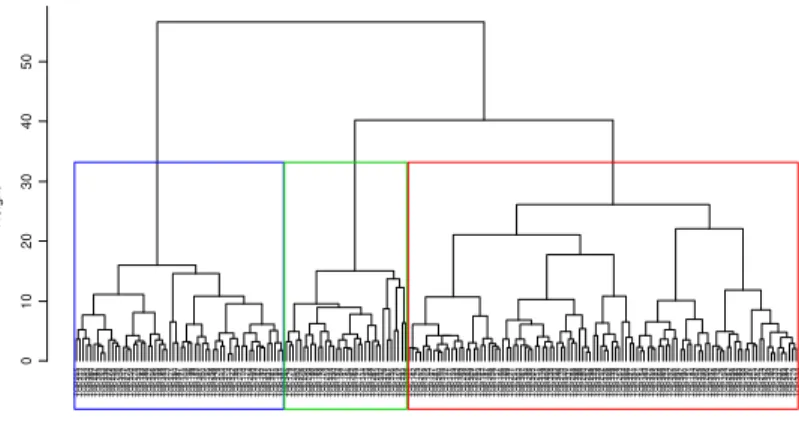
Figure 1: Dendrogram representing queries clustering.
The dendrogram in figure 1 can be cut at any level. The cutting level generally corresponds to a height where two successive nodes are clearly separated. Many relevant cutting choices can be made here (3, 4, or 6 nodes), but the main difference consist on cutting the cluster on the right in 1, 2 or 4 groups. We choose voluntarily to cut the dendrogram in order to obtain three clusters in a first approach. Figure 1 shows that the distance is more significant for the three first clusters. Next work will investigate the effect of the number of clusters on the efficiency of our method.
We will not present in this work the k-means method (Lebart and al, 2006). Therefore, after clustering query with AHC, we applied k-means methods (initialized with the centroid of each cluster determined by the AHC) in order to stabilize query clustering.
Principal Component Analysis applied to queries
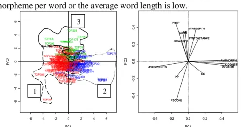
The first step when performing PCA consists in choosing the dimension of the sub-space on which projection is done. In our results, the first three PCs explain nearly half of the information (supported by 13 initial variables). From the fourth PC, the percentage of information is less than 10% and PC contains less meaningful information. Therefore, in the following, we propose the representation in the plane PC1-PC2. In figure 2, two groups of variables are opposite on the first axis: {MORPH, LENGTH, and CONJ} vs. {AVGSYNSETS}. This opposition means that if the average number of polysemy values is
important (high AVGSYNSETS), then the corresponding number of morpheme per word or the average word length is low.
-6 -4 -2 0 2 4 6 -6 -4 -2 0 2 4 6 PC1 P C 2 TOP151 TOP152 TOP153 TOP154 TOP155 TOP156 TOP157 TOP158 TOP159 TOP160 TOP161 TOP162 TOP163TOP164 TOP165 TOP166 TOP167TOP168 TOP169 TOP170 TOP171TOP172 TOP173 TOP174TOP175 TOP176 TOP177 TOP178 TOP179 TOP180 TOP181TOP182 TOP183 TOP184 TOP185 TOP186 TOP187 TOP188 TOP189TOP190 TOP191 TOP192 TOP193 TOP194 TOP195 TOP196 TOP197 TOP198 TOP199 TOP200 TOP251 TOP252TOP253 TOP254 TOP255 TOP256 TOP257 TOP258 TOP259 TOP260 TOP261 TOP262 TOP263 TOP264 TOP265 TOP266 TOP267 TOP268 TOP269 TOP270TOP271 TOP272 TOP273 TOP274 TOP275 TOP276 TOP277TOP278 TOP279 TOP280 TOP281 TOP282 TOP283 TOP284 TOP285 TOP286 TOP287 TOP288 TOP289 TOP290 TOP291 TOP292 TOP293 TOP294 TOP295 TOP296 TOP297 TOP298 TOP299 TOP300 TOP301 TOP302 TOP303 TOP304 TOP305 TOP306 TOP307TOP308 TOP309 TOP310 TOP311
TOP312TOP314TOP313
TOP315 TOP316 TOP317 TOP318 TOP319 TOP320 TOP321 TOP322 TOP323 TOP324 TOP325 TOP326 TOP327 TOP328 TOP329 TOP330 TOP331 TOP332 TOP333TOP334 TOP335 TOP336 TOP337TOP338 TOP339 TOP340 TOP341 TOP342 TOP343 TOP344 TOP345 TOP346 TOP347 TOP348 TOP349 TOP350 TOP351 TOP352 TOP353 TOP354 TOP355 TOP356 TOP357 TOP358 TOP359 TOP360 TOP361 TOP362 TOP363 TOP364 TOP365 TOP366 TOP367 TOP368 TOP369 TOP370 TOP371 TOP372 TOP373 TOP374 TOP375 TOP376 TOP377 TOP378 TOP379 TOP380 TOP381 TOP382 TOP383
TOP384TOP385TOP386
TOP387 TOP388TOP389 TOP390 TOP391 TOP392 TOP393 TOP394 TOP395 TOP396 TOP397 TOP398 TOP399 TOP400 -0.4 -0.2 0.0 0.2 0.4 -0 .4 -0 .2 0 .0 0 .2 0 .4 PC1 P C 2 NBWORDS NP ACRO PREP CC PP VBCONJ AVGSIZE AVGMORPH X.CONSTR AVGSYNSETS SYNTDEPTH SYNTDISTANCE
Figure 2: Representation of individuals (queries) and variables (linguistic features) according to PC1 and PC2
Variables and individuals that characterize query clusters can be represented in the same graph (see figure 2). In the representation of individuals (left side of the figure), the numbers we added represent clusters. According to figure 2, cluster 2 is correlated with the group of variables {MORPH, LENGTH, and CONJ}. However, how clusters are characterized by linguistic features is not the focus of this paper. Rather, we study how these clustering can be used for system recommendation.
Distribution of queries among clusters
Query clustering was computed on 200 queries from various TREC sessions. However, runs are available for each session; that means that a given system provides retrieved documents only for one session. As a result, before evaluating systems, we filter the queries according to the TREC session they belong to. The following table gives the repartition
of queries for each TREC session and for each group of queries. Nq
represents the number of queries per class.
Nq TREC3 TREC5 TREC6 TREC7
Cluster1 58 (29%) 22,41% 20,69% 29,31% 25,86%
Cluster2 34 (17%) 44,12% 29,41% 14,71% 11,76%
Cluster3 108 (54%) 19,44% 25% 26,85% 28,7%
1 2
Table 2: TREC collectionscharacteristics
Table 2 shows that cluster 3 contains 54% of the total number of queries and that 28.7% of these queries come from TREC7 data. Given these 3 clusters of queries, we evaluate system performances for each
query cluster. We use TREC’s trec_eval program used to calculate the
performance of participants’ system. Trec_eval outputs correspond to a
number of measures. We choose among them the mean average precision (MAP), R-precision, P@5, P@10, and P@15. For each of these measures, we rank systems according to their performance. This ranking is done for each session of TREC.
5 Preliminary results
In this section, we consider TREC5 data and analyze them in order to decide on the potentiality of our method.
5.1 Local evaluation (per query cluster)
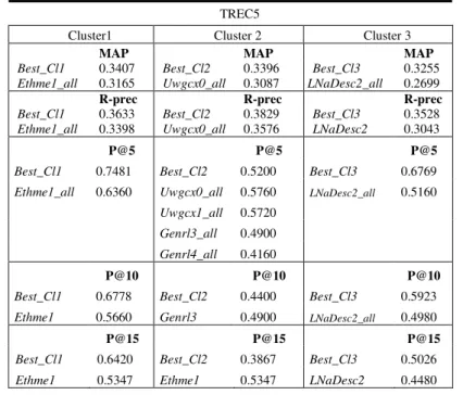
In table 3, we analyze the results we obtain for the 3 clusters in TREC5. For each measure, we report the result of the best system when averaged over the cluster‘s queries. We also report the result obtained by this system when results are averaged over the 50 queries. For
example, regarding cluster 1, Ethme1 gets the best MAP (0.3407) when
considering the queries from cluster 1. This system gets 0.3165 MAP when considering the 50 queries. It can happen that the best performance for a cluster is the same for several systems. In that case, we report the results obtained for each of these systems considering the 50 queries (e.g. P@5 for cluster2). %A represents the percentage of improvement when considering the best system within a cluster and the same system over the 50 queries.
As we can see in table 3, for the cluster 1 there is an improvement from 6.9% (R-precision) to 20% (P@15) when considering queries from cluster 1 only compared to the same system when considering all the queries. That means that system should be used for queries from cluster 1, but not for queries that does not belong to this cluster. The same type of comments can be made on cluster 3. Performance is improved from 12% up to 31% depending on the measure considered. These results show that LNaDesc2 system should be used for cluster 3. Same comments can be made regarding cluster 2 but solely for certain measures. Contrary to cluster 1 and cluster 3, for high precision in
cluster 2, the system that gets the best results in cluster 2, when considered globally over the 50 queries, performs better than on the cluster solely. That means that for this measure it is not possible to predict correctly the system to use for the queries belonging to cluster 2.
TREC5
Cluster1 Cluster 2 Cluster 3
MAP MAP MAP
Best_Cl1 0.3407 Best_Cl2 0.3396 Best_Cl3 0.3255
Ethme1_all 0.3165 Uwgcx0_all 0.3087 LNaDesc2_all 0.2699
R-prec R-prec R-prec
Best_Cl1 0.3633 Best_Cl2 0.3829 Best_Cl3 0.3528
Ethme1_all 0.3398 Uwgcx0_all 0.3576 LNaDesc2 0.3043
P@5 P@5 P@5
Best_Cl1 0.7481 Best_Cl2 0.5200 Best_Cl3 0.6769
Ethme1_all 0.6360 Uwgcx0_all 0.5760 LNaDesc2_all 0.5160
Uwgcx1_all 0.5720
Genrl3_all 0.4900
Genrl4_all 0.4160
P@10 P@10 P@10
Best_Cl1 0.6778 Best_Cl2 0.4400 Best_Cl3 0.5923
Ethme1 0.5660 Genrl3 0.4900 LNaDesc2_all 0.4980
P@15 P@15 P@15
Best_Cl1 0.6420 Best_Cl2 0.3867 Best_Cl3 0.5026
Ethme1 0.5347 Ethme1 0.5347 LNaDesc2 0.4480
Table 3: Performance of TREC5 systems on query clusters
Table 4 shows that on average, results can be improved. This table indicates column 2, the average measure over the clusters (mean of the Best_Cl1, Best_Cl2, and Best_Cl3 values. Column 3, we indicate the results the best participating system obtains (best in terms of MAP, R-precision, P@5, P@10, and P@15). In fact, the best system in term of MAP that year is also the one which gets the best results for all the measures considered.
Avg over clusters (best system for each cluster)
Best system in terms of (MAP, R-precision, P@5, P@10, P@15) MAP 0.3353 0.3070 R-Prec 0.3663 0.3444 P@5 0.6448 0.6160 P@10 0.5700 0.5460 P@15 0.5104 0.5147
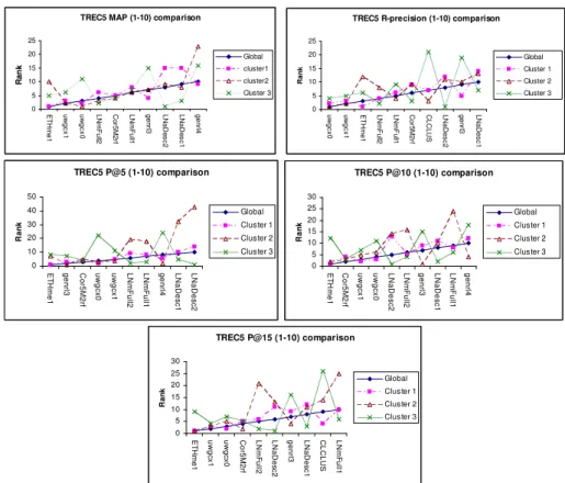
We also analyze the results from TREC5 considering the rank of the participating systems. The results are presented in figure 3.
TREC5 MAP (1-10) comparison
0 5 10 15 20 25 E T H m e 1 u w g c x 1 u w g c x 0 L N m F u ll2 C o r5 M 2 rf L N m F u ll1 g e n rl3 L N a D e s c 2 L N a D e s c 1 g e n rl4 R a n k Global cluster1 cluster2 Cluster 3
TREC5 R-precision (1-10) comparison
0 5 10 15 20 25 u w g c x 0 u w g c x 1 E T H m e 1 L N m F u ll2 L N m F u ll1 C o r5 M 2 rf C L C L U S L N a D e s c 2 g e n rl3 L N a D e s c 1 R a n k Global Cluster 1 Cluster 2 Cluster 3 TREC5 P@5 (1-10) comparison 0 10 20 30 40 50 E T H m e 1 g e n rl3 C o r5 M 2 rf u w g c x 0 u w g c x 1 L N m F u ll2 L N m F u ll1 g e n rl4 L N a D e s c 1 L N a D e s c 2 R a n k Global Cluster 1 Cluster 2 Cluster 3 TREC5 P@10 (1-10) comparison 0 5 10 15 20 25 30 E T H m e 1 C o r5 M 2 rf u w g c x 1 u w g c x 0 L N a D e s c 2 L N m F u ll2 g e n rl3 L N a D e s c 1 L N m F u ll1 g e n rl4 R a n k Global Cluster 1 Cluster 2 Cluster 3 TREC5 P@15 (1-10) comparison 0 5 10 15 20 25 30 E T H m e 1 u w g c x 1 u w g c x 0 C o r5 M 2 rf L N m F u ll2 L N a D e s c 2 g e n rl3 L N a D e s c 1 C L C L U S L N m F u ll1 R a n k Global Cluster 1 Cluster 2 Cluster 3
Figure 3: Comparison between systems’ rank when computed over all queries and rank obtained when clustering queries in 3 clusters.
In figure 3, systems are ranked according to their performances and ordered by rank for each cluster of queries and all the queries (“Global” label). We consider only the 10 best systems in term of the measure
analyzed. In this figure, ETHme1 system is the best system for the
MAP, P@5, P@10, and P@15 measures averaged over the 50 queries.
However, using ETHme1 system for queries belonging to cluster 3
makes the performance decreases. We draw the same conclusions for
ETHme1 for cluster 2 for MAP and P@5 measures. Therefore, we can
say that using ETHme1 system for the R-precision measure in cluster 2
would be relevant as performance increases: ETHme1 goes from rank three to rank one and become the best system to use in this case. In the next table, we show the percentages of correct prediction of the system to use, incorrect prediction, and prediction which do not have impact on
systems ranking. We consider a correct prediction a prediction that decreases the rank of a system (the smallest, the best). When considering figure 3, this corresponds to systems that are under the global performance line.
5.2 Global evaluation
Experiments presented section 5.2 compare the performances of the systems for a given cluster of queries to those of the systems computed on all the queries.
0 0,1 0,2 0,3 0,4 0,5 0,6 0,7 MAP R-Prec P@5 P@10 P@15 Best_Cl ETHme1 LNaDesc2 uwgcx0 genrl3 genrl4 uwgcx1
Figure 4: Global comparison of system performanceon TREC5 data.
In figure 4, we compare the system we select for the retrieval (Best_Cl) to each of the best systems for each cluster. We compute the average performance of the best systems for a measure (MAP, R-precision, P@) to get a global idea of the efficiency of our selected system (best_Cl is the average over best_Cl1, best_Cl2 and best_Cl3 for a given measure). For the 61 systems we have tested, Best_Cl achieves better than the other systems for the MAP, R_Precision, P@5 and P@10 measures. For the last measure (P@15), the system Ethme1 performs better than Best_Cl. For TREC5, we show that we are able to detect about 98.36% of the best system to use for a measure.
6 Evaluation
The analysis presented in section 5 corresponds to a first step in our experiments since it just analyses the results we could obtained if we
were able to chose a cluster of each query. In this section, we evaluate our hypothesis in a training/testing mode. We use the training mode to learn query classification and system detection for each cluster, and the testing mode to evaluate the classification and detection process.
6.1 Training/testing principle
We base our evaluation on a training/testing method. Our training sets consist of 180 queries and the 20 remaining queries are used for testing. Training and testing queries are randomly selected among all the queries (200 queries) and this is done during 10 iterations.
6.2 Results
Local evaluation (per query cluster)
Table 6 shows the repartition of the testing queries into the clusters over the years and iterations.
TREC3 TREC5 TREC6 TREC7 Average
Cluster1 8.00% 14.00% 12.50% 11.50% 11.50%
Cluster2 8.50% 5.50% 10.50% 9.00% 8.38%
Cluster3 8.00% 5.50% 2.00% 4.00% 4.88%
Table 6: Testing queries repartition among clusters
In average, cluster1 contains the higher number of queries. Calculating the proportion of the number of testing queries compare to the number of training queries, we can say that the repartition on the previous table is correct (cf. table 6) as training queries are used to determine clusters. Global evaluation
We measure here the performance of the system we select for the retrieval process by averaging the results obtained by best_Cl over the 3 clusters in order to make them comparable to the systems that participate at TREC. The first result of this global comparison shows the number of systems having higher (or smaller or equal) performance than the average performances over clusters.
Like in the previous section Best_Cl is an average over the three clusters (average of best_Cl1, best_Cl2, and best_Cl3).
TREC3 TREC5 TREC6 TREC7 Average #sys > best_Cl 19.21% 20.58% 10.26% 14.85% 16.22% #sys < best_Cl 67.55% 61.75% 80.63% 74.42% 71.09% #sys = best_Cl 13.24% 17.67% 9.11% 10.73% 12.69%
Table 7: average amelioration over clusters after “testing” queries have been affected to clusters.
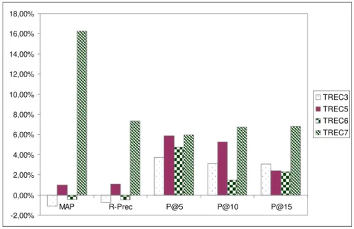
We measure in figure 5 the performances we would obtain if best_Cl was used instead of the best system for each TREC campaign. By analyzing this figure, it’s interesting to use best_Cl for all the high precision measures (P@5, P@10, and P@15). If we look at the MAP, the difference between the higher (16.27%) and lower value (-1.08%) is about 17.35%. Therefore, Best_Cl does not improve the performance of the retrieval for TREC3 and TREC6. Indeed, for TREC3, the best system is inq102. this system has a MAP value of 0.4226 whereas best_Cl obtains a score of 0.4181. For the other measures, best_Cl outperforms the best systems performances except for the MAP measure of TREC6 and the R-Precision measure of TREC3 and TREC6. -2,00% 0,00% 2,00% 4,00% 6,00% 8,00% 10,00% 12,00% 14,00% 16,00% 18,00% MAP R-Prec P@5 P@10 P@15 TREC3 TREC5 TREC6 TREC7
Figure 5: Global comparison with best_Cl system
We have done some experiments with the combMNZ method and we present in the next tab a summary of 3 systems.
MAP R_Prec P@5 P@10 P@15 combz 0,4243 inq102 0,4524 best_Cl 0,7882 best_Cl 0,7447 combz 0,7293 inq102 0,4226 best_Cl 0,4491 combz 0,776 combz 0,742 best_Cl 0,7077
Trec3 best_Cl 0,4181 combz 0,4438 brkly7 0,76 inq102 0,722 inq102 0,6867 combz 0,3186 best_Cl 0,3481 best_Cl 0,6522 best_Cl 0,5748 best_Cl 0,5272
best_Cl 0,31 uwgcx0 0,3444 ETHme1 0,616 ETHme1 0,546 ETHme1 0,5147
Trec5 ETHme1 0,307 combz 0,3436 combz 0,596 combz 0,514 combz 0,488 uwmt6a0 0,4631 uwmt6a0 0,4896 best_Cl 0,7457 best_Cl 0,6921 best_Cl 0,6534
best_Cl 0,4611 best_Cl 0,4872 CLAUG 0,712 uwmt6a0 0,682 uwmt6a0 0,6387
Trec6 combz 0,3344 combz 0,3561 combz 0,616 combz 0,538 combz 0,4853
best_Cl 0,4304 best_Cl 0,4714 best_Cl 0,8054 best_Cl 0,7407 best_Cl 0,7064
CLARIT98 COMB 0,3702 t7miti1 0,4392 CLARIT9 8CLUS 0,76 CLARIT9 8CLUS 0,694 CLARIT9 8COMB 0,6613 Trec7 combz 0,3203 combz 0,3375 combz 0,636 combz 0,598 combz 0,5387
Table 8: comparison between best_Cl, combMNZ and best systems for
TREC3, 5, 6, and 7.
In table 8, we compare the results obtained by using combMNZ method, the results obtained by best_Cl, and finally the result of the best system for each TREC campaign. If we look the MAP for TREC 3, using a fusion technique (here combMNZ with a MAP of 0.4243) gives better results than both the best system (0.4226) of TREC 3 for the MAP and best_Cl (0.4181). we can say that in general, best_Cl outperforms combMNZ and the best system for high precision.
7 Conclusion
In this paper, we make the hypothesis that queries can be clustered according to some linguistic features. We also make the hypothesis that it is possible to associate a system to use for each cluster. To evaluate this hypothesis, our analysis is two steps: we first consider the results we would obtain if we were able to choose which system to use for a category of queries. System selection (recommendation) is made on the basis of the MAP, R-precision, and P@ measures and of query clusters. Query clusters are obtained using linguistic features to represent the queries. When assuming we known how to select the best system to use for a category of query, we show that we obtain significant improvement of the results. In the second step of our study, we evaluate the hypothesis using a training/testing mode. We found that results can be improved compared to the best system among the systems that participate to TREC.
In future works, we will consider other features than only the selected linguistic-based query features. One track will be to combine query features with retrieved and relevant document set. In previous studies in the field of data fusion, it has been shown that these features associated to retrieval can be of importance for data fusion results. We will study to what extend these features can be included in a training process and how good they are to predict the best system to use.
References
Beitzel, S.M., Jensen, E.C., Chowdhury, A., Grossman, D., Frieder, O., Goharian N. (2004): Fusion of Effective retrieval strategies in the same information retrieval system. J. Am Soc. Inf. Sci. Technol., 55(10): 859-868 Buckley, C. (2004): Why current IR engines fail In Proceedings of the 27th annual International ACM SIGIR conference on Research and development in information retrieval. ACM Press, 584-585
Buckley, C., Harman, D. (2004): Reliable information access. Final report, 27th International ACM SIGIR Conference on Research and Development in Information Retrieval. Shefield: ACM Press, 528 - 529
Buckley C., Waltz J. (2000): SMART in TREC 8. In The Eighth Text REtrieval Conference
(TREC-8). Ed. E.M. Voorhees and D.K. Harman. Gaithersburg, MD: NIST. Buscaldi, D., Rosso, P., Sanchis Arnal, E. (2005): A WordNet-based Query
Expansion method for. Geographical Information Retrieval, CLEF,
http://www.clef-campaign.org/2005/working\_notes/workingnotes2005/buscaldi05.pdf. Chang, Y., Kim, M., Ounis, I. (2004): Construction of query concepts in a
document space based on data mining techniques. Proceedings of the 6th International Conference On Flexible Query Answering Systems (FQAS,2004). Lecture notes in Artificial Intelligence, Lyon, France, June 24-26, 137-149
Cronen-Townsend, S., Zhou, Y., Croft, W.B. (2002): Predicting query performance. Proceedings of the 25th annual international ACM-SIGIR conference on research and development in information retrieval, Tampere, 299-306
Fabre, C., Bourigeault, D. (2001): Linguistic clues for corpus-based acquisition of lexical dependencies, in Proceeding of Corpus Linguistics, Lancaster
Fox, E.A., Shaw, J.A. (1994): Combination of multiple searches. Proceedings of the 2nd Text Retrieval Conference (TREC-2), NIST special publication, 243-252
Lebart, L., Morineau, A., Piron, M. (2006): Statistique exploratoire multidimensionnelle : Visualisations et inférences en fouille de données. 4ème édition, Dunod, Paris, 6 juillet 2006
Lee, J. (1997): Analysis of multiple evidence combination. 22th International ACM SIGIR Conference on Research and Development in Information Retrieval. New York: ACM Press, pp. 267-276
Mandl, Womser-Hacker, T. (2003): Linguistic and statistical analysis for the CLEF topics. Peters C, Braschler M, Gonzalo J and Kluck M, Eds. Advances in Cross-Language Information Retrieval: Results of the CLEF 2002 Evaluation Campaign, LNCS 2785. Spinger Verlag, 505-511
Mardia, K.V., Kent, J.T., BIbby, J.M. (1989): Multivariate Analysis. Academic Press.7th Printing.
Mothe, J.,Tanguy, L. (2005): Linguistic features to predict query difficulty- A case study on previous TREC campaigns SIGIR workshop on Predicting Query Difficulty - Methods and Applications.