Informed Trading and
Expected Returns
James J. Choi
Yale School of Management and NBER Li Jin
Oxford University Saïd Business School and Peking University Guanghua School of Management
Hongjun Yan
Yale School of Management
March 1, 2013
Abstract
Does information asymmetry affect the cross-section of expected stock returns? Using institutional ownership data from the Shanghai Stock Exchange, we show that institutions have a strong information advantage over individual investors. We then show that the aggressiveness of institutional trading in a stock—measured by the average absolute weekly change in institutional ownership during the past year—is an ex ante predictor of future information asymmetry in this stock. Sorting stocks on this information asymmetry predictor, we find that the top quintile outperforms the bottom quintile next month by 10.8% annualized, suggesting that information asymmetry raises the cost of capital.
*
We thank seminar audience members at Cheung Kong GSB, Hong Kong University, HKUST, the University of Toronto, and Yale for their insightful comments.
Does information asymmetry affect the cross-section of expected stock returns? The theoretical literature has come to different conclusions. Easley and O’Hara (2004) argue that stocks with more information asymmetry should have higher expected returns to compensate uninformed investors for the losses they suffer from trading against informed investors. Their model shows that, holding the total quantity of information constant, stocks with more private information have a higher return premium. However, Hughes, Liu, and Liu (2007) argue that the relationship between information asymmetry and expected returns disappears in large economies because of diversification. Lambert, Leuz, and Verrecchia (2011) argue that, holding the average precision of investors’ beliefs about a stock’s fundamental value constant, a positive relationship between information asymmetry and expected returns arises only in financial markets where investors are not price-takers. Models with only one risky asset provide intuitions that information asymmetry might affect the cross-section of expected returns through its effects on liquidity, the usefulness of an asset for risk-sharing, and the risk-bearing capacity available through market makers, but the sign of the predicted relationship differs both within and across models.1
Empirical tests of the cross-sectional relationship between information asymmetry and expected returns have to overcome the difficulty of identifying stock-level variation in information asymmetry.2 In this paper, we identify information asymmetry using a unique dataset that contains the daily stock holdings of a representative sample of all Shanghai Stock Exchange investors. Our setup has two advantages. First, the high frequency and representative nature of our sample allows us to more accurately measure the prevalence of informed trading than in most other markets, where ownership data are either available only at much lower frequencies or come from a non-representative investor sample. Second, due to the less-developed state of Chinese legal institutions and regulations, there is likely to be greater cross-sectional variation in how much private information is shared with selected outside investors
1 See Diamond and Verrecchia (1991), Gârleanu and Pedersen (2004), and Vayanos and Wang (2012).
2 See Neal and Wheatley (1998) and Van Ness, Van Ness, and Warr (2001) for evidence that measures of adverse
than in developed markets, where a stricter regulatory environment compresses the amount of information asymmetry among active traders towards zero. This greater variation gives our analysis more statistical power to detect information asymmetry effects on returns. Chinese stock returns share many features of developed stock returns—for example, during our sample period, size, book-to-market, and momentum effects are present in the Shanghai Stock Exchange— suggesting that return phenomena in China offer insights into returns in other markets as well.3
We first identify one large group of investors in the Shanghai Stock Exchange that has an information advantage: institutions. If each week during our 1996 to 2007 sample period, one bought stocks whose institutional ownership percentage change in the prior week was in the top quintile and sold short stocks whose institutional ownership change in the prior week was in the bottom quintile, the resulting four-factor portfolio alpha was 129 basis points per month, or 15.5% per year, and significant at the 1% level (t = 5.88).
To examine the effect of information asymmetry on the cross-section of expected returns, we need to construct an ex ante predictor of future information asymmetry for each stock. We conjecture and confirm that institutions’ future information advantage is larger in stocks in which they have previously traded more aggressively.4 Our conjecture is motivated by the intuition that institutions’ trades in stocks where they have no information advantage are primarily caused by their need to invest customer asset inflows and meet liquidity demands, whereas institutional trades in stocks where they have an information advantage are additionally driven by value signals that are largely orthogonal to asset inflows and liquidity needs. Therefore, the volatility
3
Chen et al. (2010) test 18 variables that have been shown to predict cross-sectional stock returns in the U.S. market and find that in the 1995 to 2007 period, all 18 variables’ point estimates in univariate Fama-MacBeth (1973) regressions have signs consistent with the U.S. evidence, and five are statistically significant, compared to eight significant coefficients for the U.S. markets during this same period.
4
We have also tried using the past year’s institutional trading profits (as defined later in this paper) in a stock as a predictor of future information asymmetry. The results of this alternative analysis are consistent with those reported in the paper: portfolios with higher predicted future information asymmetry have higher future alphas in the cross-section. We do not use past trading profits as our main predictor because its relationship with future information asymmetry is non-monotonic—both stocks with very high and very low past institutional trading profits have higher future information asymmetry than stocks with moderate past institutional trading profits—making the use of this variable expositionally inconvenient. Intuitively, if an investor has more precise information about a stock, she will set up a more aggressive position in the stock, and her realized trading profit will be either very high or very low.
of institutional ownership should be higher in stocks where institutions have a greater information advantage. If in addition, stocks in which institutions have had private information in the past are more likely to be stocks in which institutions will have private information in the future, then past institutional ownership volatility will predict future institutional information advantage.
At each month-end, we construct our predictor of future information asymmetry for stock
i as the average weekly absolute change in i’s institutional ownership percentage over the most recent fifty weeks, which we will refer to as “prior institutional ownership volatility.” We confirm that this sorting variable creates a spread in future information asymmetry by using it to predict future institutional trading profits in the stock. Controlling for stock characteristics, institutions’ trading profits should be increasing in their information advantage. We compute institutional trading profit in stock i during week t as (i’s return in excess of the market during week t) × (the change in i’s institutional ownership percentage during week t – 1 in excess of the average stock’s institutional ownership percentage change in week t – 1). We find that institutions’ average weekly trading profit during the following month increases with prior institutional ownership volatility, indicating that our sorting variable indeed creates a spread across stocks in future information asymmetry.5
Having established the validity of our predictor of information asymmetry, we conduct our main cross-sectional return test. Consistent with information asymmetry increasing the cost of capital, we find that stocks in the top quintile of prior institutional ownership volatility have a four-factor alpha that is 90 basis points higher per month (10.8% annualized) than that of their bottom-quintile counterparts, a difference that is significant at the 1% level (t = 3.51).
Examining the results separately by market capitalization tercile, we find that even though institutions have an information advantage in all size terciles, sorting on our predictor, prior institutional ownership volatility, creates a spread in future institutional information
5 Our measure does not capture trading profits by informed individuals. To the extent that informed individuals
advantage only among large and mid-cap stocks, not among small stocks. This variation provides a useful placebo test. If our sort creates a spread in expected returns among small stocks, then we might be concerned that some omitted variable correlated with prior institutional ownership volatility, rather than future information asymmetry, is responsible for the relationship between prior institutional ownership volatility and expected returns in the full sample. Instead, we find that there is no significant expected return difference (t = 0.45) between the top and bottom quintiles of prior institutional ownership volatility among small stocks. In contrast, the expected return difference between the extreme quintiles is large and significant at the 1% level among mid-cap stocks (t = 4.44) and large-cap stocks (t = 4.92), where prior institutional ownership volatility does create a spread in future institutional trading profits.
Prior institutional ownership volatility’s ability to predict returns is persistent. The difference between the top and bottom quintile alphas is significant for ten months after the initial sorting month, with no evidence of return reversals. Interestingly, we find that prior institutional ownership volatility also predicts institutional trading profits for ten months after the initial sorting month. This congruence between alpha persistence and institutional trading profit persistence is further evidence that information asymmetry is responsible for the expected return variation created by our prior institutional ownership volatility sort.
In robustness checks, we find that liquidity and price pressure from future institutional buys and sells are not responsible for our main results. In fact, stocks in the top quintile of prior institutional ownership volatility are more liquid and experience less institutional buying during the month after portfolio formation than stocks in the bottom quintile, both of which act to lower
the top quintile’s returns.
Our paper contributes to the literature that tries to empirically identify the impact of information asymmetry on the cross-section of expected stock returns. Easley, Hvidkjaer, and O’Hara (2002) use the temporal clustering of buy and sell orders to estimate the probability of informed trading (PIN) and find that high-PIN stocks have higher returns than low-PIN stocks. However, Duarte and Young (2009) argue that PIN is priced due to its correlation with liquidity rather than information asymmetry, a claim that Easley, Hvidkjaer, and O’Hara (2010) dispute.
Mohanram and Rajgopal (2009) argue that the PIN-return relationship is not robust to alternative specifications and time periods, while Aslan et al. (2011) argue the opposite. Kelly and Ljungqvist (2012) use exogenous changes in sell-side analyst coverage to identify changes in information asymmetry. They find that stock prices drop when sell-side analyst coverage decreases.6
Our paper is distinguished from these prior studies in that we directly observe the presence and activity of informed traders in each stock, rather than inferring them from proxies. In this sense, our approach is closest to that of Berkman, Koch, and Westerholm (forthcoming), who use Finnish data to show that trades executed through children’s accounts are unusually successful, indicating that the children’s guardians are informed. They construct a measure called BABYPIN that is the proportion of trading activity in a stock that occurs through children’s accounts, and find that high BABYPIN stocks have higher returns. However, due to the small size of the Finnish stock market, the average number of stocks in their cross-sections is only 46. Therefore, they are unable to address the theoretical argument of Hughes, Liu, and Liu (2007) that the effect of information asymmetry will disappear in large economies. In our data, the average number of stocks in a given year is 573, so our estimates should reflect most of the effects of diversification.
Our paper proceeds as follows. Section I gives a brief background on the Shanghai Stock Exchange. Section II describes our data, and Section III establishes that institutions have an information advantage when they trade. Section IV details our methodology for constructing an
ex ante predictor of information asymmetry and validates this predictor. Section V contains our main empirical test of whether greater information asymmetry increases expected returns, and Section VI runs these tests separately by market capitalization tercile. Section VII examines the persistence of abnormal returns and institutional information advantage after the portfolio formation month. Section VIII contains robustness checks, and Section IX concludes.
6 Balakrishnan et al. (2012) find evidence that, in response to the decrease in analyst coverage, firms attempt to
I. Background on the Shanghai Stock Exchange
At the end of 2007—the last year of our sample period—the 860 stocks traded on the Shanghai Stock Exchange (SSE) had a total market capitalization of $3.7 trillion, making it the world’s sixth-largest stock exchange behind NYSE, Tokyo, Euronext, Nasdaq, and London. Mainland China’s other stock exchange, the Shenzhen Stock Exchange, had a $785 billion market capitalization at year-end 2007. At year-end 2011, mainland China’s collective stock market had the second-largest market capitalization among all countries of the world, behind only the U.S.
Almost all SSE shares are A shares, which only domestic investors could hold until 2003. At year-end 2007, A shares constituted over 99% of SSE market capitalization. B shares are quoted in U.S. dollars and can be held by foreign and (since 2001) domestic investors. Shares are further classified into tradable and non-tradable shares. Non-tradable shares have the same voting and cashflow rights as tradable shares and are typically owned directly by the Chinese government (“state-owned shares”) or by government-controlled domestic financial institutions and corporations (“legal person shares”). We use the term “tradable market capitalization” to refer to the value of tradable A shares, and “total market capitalization” to refer to the combined value of tradable and non-tradable A shares. During our sample period, about 27% of SSE market capitalization was tradable.7
There is minimal equity derivatives activity in the Chinese markets. Prior to the end of 2005, there were no equity derivatives at all. From 2005 to 2007, eleven SSE companies were allowed to issue put warrants (Xiong and Yu, 2011). Therefore, nearly all trading on company information must happen via the stock market. Short-sales were not allowed during our sample
7
Beginning in April 2005, non-tradable shares began to be converted to tradable status, but the conversion process was slow enough that as of year-end 2007, only 28% of total Chinese market capitalization was tradable. Converted tradable shares were subject to a one-year lockup, and investors holding more than a 5% stake were subject to selling restrictions for an additional two years.
period, so whenever we refer to “shorting” a portfolio, it should be understood as a hypothetical position.
II. Data description
We obtain stock return, market capitalization, and accounting data from the China Stock Market & Accounting Research Database (CSMAR).
Our daily ownership data come from the SSE. To trade stocks listed on the SSE, both retail and institutional investors are required to open an account with the Exchange, at which point they must identify themselves to the Exchange as an individual or an institution. Each account uniquely and permanently identifies an investor, even if the account later becomes empty. Investors cannot have multiple accounts. The data assembled by the Exchange for this paper consists of the entire history of SSE tradable A share holdings from January 1996 to May 2007 for a representative random sample of all accounts that existed at the end of May 2007.8 Since there are far fewer institutional accounts than retail accounts, the Exchange over-sampled institutional investors in order to ensure that a meaningful number of institutional accounts were extracted. The stock-level statistics computed from these account data are reweighted to adjust for the over-sampling of institutional investors.
The sample contains both currently active and inactive accounts, so there is no survivorship bias, and in expectation, a constant fraction of the accounts extant at any date are represented. The number of accounts in the sample grows from 36,349 retail accounts and 360 institutional accounts to 384,709 retail accounts and 20,727 institutional accounts from January 1996 to May 2007. Holdings data are aggregated at the Exchange into daily stock-level institutional ownership percentage measures. The aggregation is carried out under arrangements that maintain strict confidentiality requirements to ensure that no individual account data are disclosed. The institutional ownership series are not disclosed to the public, so they cannot be used for actual trading.
Table 1 shows year-by-year summary statistics on the fraction of tradable A shares owned by institutions. Over our sample period, the weight of the SSE investor base has shifted from individuals to institutions. From 1996 to 2007, institutional ownership in the average stock rose from 4.3% to 19.2%, and the across-stock standard deviation in institutional ownership rose from 9.3% to 24.9%. Weighting across stocks by tradable market capitalization, the average institutional ownership grew even more quickly—from 4.6% to 46.7%—indicating that the expansion of institutional ownership occurred disproportionately in large stocks. The number of stocks in our sample rises from 186 to 802.9
III. Do institutions have an information advantage?
We begin our analysis by establishing that institutions have an information advantage. We do this by showing that stocks that institutions have bought heavily subsequently outperform stocks that institutions have sold heavily. Our objective is not to necessarily extract the maximum possible amount of information from institutional trades, but rather to show that one simple approach—among many possible approaches—successfully predicts future returns, which is sufficient to demonstrate institutions’ informational advantage.
At the end of each Friday that is a trading day, we compute the change in institutional ownership percentage since the end of the prior Friday that was a trading day.10 We sort stocks into quintile portfolios based on this change, weight them by their tradable market capitalization, and hold them until the end of the next Friday that is a trading day. Henceforth, we will refer to a trading Friday to trading Friday period as a “week,” even though market holidays sometimes make this period longer than seven days.11
9 The number of stocks in our sample is slightly smaller than the total number of SSE stocks because of gaps in
CSMAR’s coverage.
10 We compute the difference, not the difference as a proportion of the initial ownership level. In other words, a
change from 20% to 21% is a 1% change.
11 We use ownership percentage differences and a weekly frequency in order to be consistent with our later
definition of institutional excess trading profits. Choi, Jin, and Yan (forthcoming) show that monthly log institutional ownership percentage changes predict the subsequent month’s return in the SSE.
The first five columns in Panel A of Table 2 show the average raw monthly returns of these portfolios in excess of the demand deposit rate, which we use as our riskfree return proxy. The four portfolios holding the bottom 80 percentiles of institutional ownership change stocks have excess returns between 1.47% and 1.85% per month, but there is no clear trend across the portfolios. The top quintile portfolio’s average excess return of 3.13% per month is markedly higher than the rest. The last column shows that the difference between the top and bottom quintile portfolios’ excess raw returns is 1.49% per month and significant at the 1% level (t = 6.91). Judging from the pattern of raw returns, it appears that heavy buying by Chinese institutions (i.e., being sorted into the top quintile) is a signal of good news, but anything from heavy selling to moderate buying by institutions (i.e., being sorted into the bottom four quintiles) has little information content about future returns. The absence of low returns following institutional sales could be due to corporate insiders being more reluctant to share negative news than positive news privately with outsiders and/or institutional sales being predominantly driven by liquidity needs orthogonal to information.12
We estimate the institutional ownership change portfolios’ one-, three-, and four-factor alphas by regressing their monthly excess returns on monthly factor portfolio returns that capture CAPM beta, size, value, and momentum effects. The market portfolio excess return is the composite Shanghai and Shenzhen market return, weighted by tradable market capitalization, minus the demand deposit rate. We construct size and value factor returns (SMB and HML, respectively) for the Chinese stock market according to the methodology of Fama and French (1993), but using the entire Shanghai/Shenzhen stock universe to calculate percentile breakpoints. We form SMB based on total market capitalization and HML based on the ratio of book equity to total market capitalization, weighting stocks within component sub-portfolios by
12 Hong, Lim, and Stein (2000) have also hypothesized that corporate managers would be more reluctant to share
bad news. Han and Hirshleifer (2012) hypothesize that individual investors are more likely to talk about their investing successes than their investing failures. Jeng, Metrick, and Zeckhauser (2003) find that corporate insiders do not earn abnormal returns on their company stock sales, but they do earn abnormal returns on their own-company stock purchases.
their tradable market capitalization.13 We construct the momentum factor portfolio MOM following the methodology described on Kenneth French’s website. We calculate the 50th percentile total market capitalization at month-end τ – 1 and the 30th and 70th percentile cumulative stock returns over months τ – 12 to τ – 2, again using the entire Shanghai/Shenzhen stock universe to calculate percentile breakpoints. The intersections of these breakpoints delineate six tradable-market-capitalization-weighted sub-portfolios for which we compute month τ returns. MOM is the equally weighted average of the two recent-winner sub-portfolio returns minus the equally weighted average of the two recent-loser sub-portfolio returns.
The alphas are consistent with the story suggested by the raw returns.14 There are no significant abnormal returns for the portfolios containing the bottom 80 percentiles of institutional ownership change stocks. The top quintile portfolio has alphas that are large and significant at the 1% level: one-, three-, and four-factor alphas of 1.14%, 1.33%, and 1.32% per month with t-statistics of 4.87, 6.19, and 6.14, respectively. The alphas of the portfolio that buys the top-quintile portfolio and shorts the bottom-quintile portfolio are similar in magnitude and statistical significance: one-, three-, and four-factor alphas of 1.38%, 1.29%, and 1.29% per month with t-statistics of 6.32, 5.91, and 5.88.
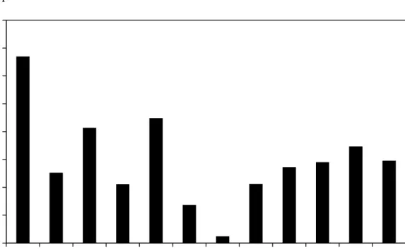
Figure 1 plots the average raw monthly return of the long-short portfolio by calendar year. The average return during the 2002-2007 period is lower than the average return during the 1996-2001 period—1.17% versus 1.78%—perhaps indicating stricter regulation of disclosure and stricter enforcement of these regulations.
We repeat the above analysis separately by size tercile. At the end of each week, we independently sort stocks into terciles based on tradable market capitalization and quintiles based on their institutional ownership percentage change since the end of the prior week. Stocks within each portfolio are weighted by their tradable market capitalization and held until the end of the
13
Whenever possible, we use the book equity value that was originally released to investors. If this is unavailable, we use book equity that has been restated to conform to revised Chinese accounting standards.
14 The alphas need not average to zero because our test portfolios are composed entirely of Shanghai Stock
following week. Table 3 reports, separately for each size tercile, the monthly raw excess return and alphas of long-short portfolios that hold the highest institutional ownership change quintile portfolio long and the lowest institutional ownership change quintile portfolio short.
We find that institutions have a strong information advantage in every size tercile. The raw long-short returns and one-, three-, and four-factor alpha spreads are significant at the 1% level for all size groups, with t-statistics of 3.95 or above. The magnitudes of the alpha spreads are large. For example, the four-factor alpha spread is 1.54% per month for small-caps, 1.55% per month for mid-caps, and 1.20% per month for large-caps.
IV. Predicting stock-level information asymmetry
Section III showed that institutions have an information advantage on average across stocks. In this section, we identify in which stocks institutions have a greater information advantage going forward. We conjecture and confirm that the aggressiveness of past institutional trades in a stock is a good predictor of institutions’ future information advantage in that stock. Our measure of institutional trading aggressiveness is prior institutional ownership volatility— the average of the 50 most recent weekly absolute institutional ownership percentage changes in the stock.15 On the last trading Friday of each month, we sort stocks into quintiles based on this measure.
Table 4 displays summary statistics for the stocks in each prior institutional ownership volatility quintile. Because the number of stocks listed on the SSE expanded rapidly during our sample period, we calculate at each month-end the mean of each variable and report the time-series average of these monthly means in order to keep later time periods from dominating the summary statistics.
15 Results are similar if we de-mean weekly institutional ownership percentage change before taking the absolute
value. That is, if our lookback window is weeks -1 to -50, compute the average signed weekly institutional ownership change over -1 to -50. Subtract this average from each weekly institutional ownership change in the lookback window. Take the absolute value of each de-meaned institutional ownership change from -1 to -50, and compute their average.
Stocks in the bottom quintile on average experienced only a 0.05% weekly absolute change in institutional ownership during the prior 50 weeks, while stocks in the top quintile experienced an average absolute change of 1.52%. Institutional ownership levels are increasing in prior institutional ownership volatility, which is consistent with the theoretical prediction that
on average, informed traders should have larger stakes in the stocks where they have more precise information, since their subjective uncertainty about these stocks is lower.16 A number of stock characteristics associated with lower expected returns in the U.S. are associated with higher prior institutional ownership volatility: large size, low book-to-market, high prior-month turnover, and high Amivest liquidity ratio (measured as the sum of the stock’s yuan trading volume over one month divided by the sum of the stock’s absolute daily returns over that month; higher values correspond to lower price impacts of trading, and hence higher liquidity). On the other hand, recent returns, which are positively correlated with expected returns in the U.S., are increasing in prior institutional ownership volatility.17
The correlation between institutional ownership volatility and the above stock characteristics suggests that institutions choose to invest more heavily in acquiring information about certain types of companies. Many of these characteristics significantly predict SSE stock returns during our sample period in a direction consistent with the U.S. patterns, so it will be important to control for them in our cross-sectional return tests. In an untabulated Fama-MacBeth (1973) regression that includes all stocks for which we can compute prior institutional ownership volatility, we find that the log of total market capitalization and turnover negatively predict next month’s returns at the 1% significance level, book-to-market positively predicts next
16 Suppose both the informed and uninformed investors are mean-variance optimizers. If both investors have the
same estimate of a stock’s expected return, the informed investor will hold more of this stock due to her lower subjective uncertainty. Although an informed investor may overweight or underweight any given stock due to her private signal, her average holdings (across time and across assets) in stocks where she has an information advantage will be higher than an uninformed investor’s (see, for example, Van Nieuwerburgh and Veldkamp, 2006).
17
The U.S. return evidence is reported in, among many other places, Fama and French (1992), Jegadeesh and Titman (1993), Haugen and Baker (1996), and Amihud (2002). Amihud (2002) uses an illiquidity measure that is highly correlated with the Amivest measure. We prefer the Amivest measure over the Amihud (2002) measure in the Chinese markets because the SSE’s daily price movement limits may distort the Amihud measure.
month’s returns at the 1% significance level, prior eleven-month return lagged one month positively predicts next month’s returns at the 5% significance level, and prior-month return and the Amivest liquidity ratio have no significant predictive power.
We now verify that prior institutional ownership volatility in a stock is indeed a good predictor of institutions’ future information advantage in the stock. In both the monopolistic setting of Kyle (1985) and the competitive setting of Easley and O’Hara (2004), informed trader profits are increasing in his/their information advantage. Therefore, we check whether prior institutional ownership volatility predicts future institutional trading profits in the stock.18 Controlling for stock characteristics, expected institutional trading profits should be increasing in institutional information advantage.
Let 𝑅𝑖𝑡 be stock i’s return during week t, 𝑅𝑚𝑡 be the market return during week t, and
Δ𝑞𝑖𝑡 be the change in the percent of tradable A shares owned by institutions in stock i from the end of week t – 1 to the end of week t. Let Δ𝑞�𝑡= (∑ Δ𝑞𝑖 𝑖𝑡)/𝐼𝑡, where 𝐼𝑡 is the total number of stocks in our sample at week t. We compute institutional trading profit in stock i during week t as (𝑅𝑖𝑡− 𝑅𝑚𝑡)(Δ𝑞𝑖,𝑡−1− Δ𝑞�𝑡−1).19 This expression corresponds to the extra profit (as a fraction of
i’s tradable market capitalization at the end of week t) institutions accrued during week t because of their net trades in i during week t – 1 in excess of their average net trades across all stocks during t – 1, assuming that the alternative investment was the market portfolio and that
18 An alternative ex post measure of information advantage is the slope coefficient from regressing future returns on
past informed trader order flow. This measure, however, is less desirable for both theoretical and empirical reasons. In Kyle (1985), for example, when the amount of noise trading increases, uninformed investors learn less from prices, so information asymmetry increases. The profit measure captures this increase in asymmetry, since the informed investor trades more aggressively and makes more profit. But the slope coefficient decreases, thus misclassifying the increase in asymmetry as a decrease. Empirically, when we sort stocks by their estimated slope coefficient from regressing week t excess returns on week t – 1 institutional ownership change, the extreme quintiles are predominantly populated by stocks in which institutions did not trade particularly actively but which experienced returns of large magnitude. The fact that institutions were relatively passive in these stocks suggests that they do not have much private information about these companies.
19
institutions held their positions at the end of t – 1 until the end of t.20 Note that this product can be positive either because institutions increased their holdings prior to a positive excess return or decreased their holdings prior to a negative excess return.
The first column of Table 5 shows results from a Fama-MacBeth regression on stock × month observations. The dependent variable is the average of weekly institutional trading profits in stock i over all weeks whose Friday is in month τ + 1. The explanatory variables are dummies for the stock’s prior institutional ownership volatility quintile as of the last trading Friday of month τ. We find that the average weekly institutional trading profit in the next month rises with prior institutional ownership volatility. The average weekly profit is 0.52 basis points higher (t = 3.53, p = 0.001) as a fraction of the stock’s tradable market capitalization in the top quintile (quintile 5) than in the bottom quintile (quintile 1). The constant term is positive but significant only at the 10% level (t = 1.83, p = 0.070), indicating that stocks in the bottom quintile have relatively symmetric information going forward. The fact that there are significantly positive institutional trading profits in the top three quintiles and none of the quintiles have negative institutional trading profits indicates that institutions have an information advantage in the average stock.
Additionally controlling for the log of tradable market capitalization, book-to-market, prior-eleven-month return lagged one month, prior-month return, prior-month turnover, and prior-month Amivest liquidity ratio as of the last trading Friday of month τ in the second column makes little difference. The top institutional ownership volatility quintile dummy coefficient rises slightly to 0.56 basis points and remains significant at the 1% level. The coefficients on the additional control variables are all statistically insignificant.
20 Although this measure only counts profits from information that is revealed in the week following the trade, it has
the advantage of not crediting institutions for returns that occur following a long passive holding period, which is less likely to be motivated by private information.
V. Do stocks with higher information asymmetry have higher expected returns?
Having shown that prior institutional ownership volatility in a stock predicts future institutional information advantage in the same stock, we now analyze the relationship between predicted institutional information advantage and expected returns. On the last trading day of each month, we sort stocks into quintiles by their prior institutional ownership volatility.21 Portfolio 1 contains stocks in the lowest 20 percentiles of prior institutional ownership volatility, and Portfolio 5 contains stocks in the highest 20 percentiles. Stocks in each portfolio are weighted by their tradable market capitalization. We hold the portfolios for one month before re-sorting stocks into new portfolios. Because we require 50 prior weeks of trading data for a stock before we include it in a portfolio, our results are not skewed by outlier first-day IPO returns.
The first four columns of Panel A in Table 6 show the raw returns in excess of the riskfree rate of each prior institutional ownership volatility portfolio. The excess returns of the bottom four quintile portfolios (1 through 4) are similar to each other, ranging from 1.27% to 1.39% per month. The top quintile portfolio has considerably higher excess returns of 1.70% per month, which is statistically distinguishable from zero. The last column shows that the difference between the top and bottom quintiles is 0.32% per month, but this is not statistically significant.
Panels B through D contain results from regressions that estimate one-, three-, and four-factor alphas for the prior institutional ownership volatility portfolios. The one-four-factor alphas for the bottom four quintile portfolios are insignificant, and despite the one-factor alpha of the top quintile portfolio being positive and significant, the difference between the top and bottom quintile alphas is not significant. However, once we control for size and book-to-market effects, the alphas rise monotonically with prior institutional ownership volatility. The bottom quintile portfolio has a significant negative three-factor alpha of 0.58% per month, and the top quintile portfolio has a significant positive three-factor alpha of 0.55% per month. The difference between the top and bottom quintile three-factor alphas is 1.13% per month and significant at the
21 We use prior institutional ownership volatility as of the last trading Friday of the month for the sort. Whereas the
analysis in Table 5 measures dependent variable returns starting after the last trading Friday of the month, our cross-sectional return analysis always measures dependent variable returns starting after the last trading day of the month.
1% level (t = 4.00). Additionally controlling for momentum yields similar results, with a four-factor alpha spread between the top and bottom quintiles of 0.90% that is significant at the 1% level (t = 3.51).
In sum, we find significantly higher abnormal returns among stocks in which we predict greater information asymmetries going forward, consistent with the hypothesis that information asymmetry increases the cost of capital.
VI. Analysis by size tercile
Many departures from the four-factor pricing model are more pronounced in small stocks, perhaps because these departures represent mispricings that are harder to arbitrage away in small stocks or because large, sophisticated institutional investors do not find it worthwhile to correct pricing errors that add up to small monetary amounts. This general pattern motivated us to examine how the relationship between prior institutional ownership volatility and expected returns varies by stock size.
We first check that prior institutional ownership volatility predicts future institutional trading profits during the next month in each size group. We independently sort stocks into terciles by tradable market capitalization and quintiles by prior institutional ownership volatility at the end of each month. Table 7 shows the results from running our Table 5 regressions, separately for each size tercile, of next month’s average weekly institutional trading profit on prior institutional ownership volatility quintile dummies as of the last trading Friday of the current month. We find that in fact, only among mid-cap and large-cap stocks does a stock’s prior institutional ownership volatility predict future information asymmetry in that stock. There is no difference in future institutional trading profits across prior institutional ownership volatility quintiles among small stocks. The lack of a trading profit spread among small stocks may be due to there being little variation in the degree of information asymmetry across small stocks; this would cause variation in past institutional trading aggressiveness to be driven almost entirely by non-informational factors. Alternatively, institutions’ information advantage in any
given small stock may be quite transitory, so that past trading behavior in a stock gives little information about future information advantage in that stock.
This null finding implies that small stocks provide a placebo test for our empirical approach. If we find a significant relationship between prior institutional ownership volatility and expected returns among small stocks, then we might be concerned that an omitted variable, rather than future information asymmetry, is responsible for the full-sample correlation between prior institutional ownership volatility and expected returns. Conversely, we might also be concerned if we do not find a significant positive relationship between prior institutional ownership volatility and expected returns among mid-cap and large-cap stocks, since prior institutional ownership volatility does create a spread in future information asymmetry in those stocks.
For our expected return tests, we form fifteen portfolios based on independent sorts of stocks at the end of each month into tradable market capitalization terciles and prior institutional ownership volatility quintiles. Stocks within each portfolio are weighted by their tradable market capitalization and held until the end of the following month, when the portfolios are reconstituted.
Table 8 shows how returns and alphas differ between the top and bottom prior institutional ownership volatility quintile portfolios within each size tercile. In the first column, we see that across raw excess returns and one-, three-, and four-factor alphas, the difference between the top and bottom quintiles is never significant among small-cap stocks, with t -statistics always less than 0.7. On the other hand, the three- and four-factor alpha spreads are large in magnitude and significant at the 1% level among and large-cap stocks. For mid-caps, the alpha spread is about 1.05% per month, and for large-mid-caps, the alpha spread is about 1.50% per month. Thus, in the size tercile where our sorting procedure does not create a spread in future information asymmetry, we find no spread in expected returns. And in the size terciles where our sorting procedure does successfully create a spread in future information asymmetry, we find a large and highly significant spread in expected returns.
VII. Persistence of expected return and information asymmetry differences across portfolios
In this section, we first explore how long alpha differences across prior institutional ownership volatility portfolios persist after portfolio formation. We form n-month-ahead portfolios by using prior institutional ownership volatility as of the last trading Friday of month τ to sort stocks into quintile portfolios at month-end τ + n – 1. Each stock is weighted in its portfolio by its tradable market capitalization as of month-end τ + n – 1. We then hold these stocks for one month before re-sorting stocks across portfolios. Table 9 shows raw returns and alphas from holding the top quintile portfolio long and the bottom quintile portfolio short. Significantly positive long-short three- and four-factor alphas persist for ten months after the quintile formation month, declining gradually with time since formation. The ten-month-ahead long-short portfolio has a three-factor alpha of 0.53% per month (t = 2.47, p = 0.015) and a four-factor alpha of 0.50% per month (t = 2.28, p = 0.024). There are no significant negative long-short alphas during the twelve post-formation months we examine, indicating that there is no reversal of the early positive alphas.
How closely does the persistence of these alpha differences match the persistence of asymmetric information differences across portfolios? Table 10 examines the ability of institutional ownership volatility to predict institutional trading profits n months ahead. We run Fama-MacBeth regressions on stock × month observations like in Table 5, with the dependent variable being the average institutional weekly trading profit in a stock over weeks whose Friday is in month τ + n and the explanatory variables being dummies for the stock’s membership in prior institutional ownership volatility quintiles as of the last trading Friday of month τ.
We find that information asymmetry that is correlated with institutional ownership volatility reverts to the mean over time. As n goes from 1 to 12, the constant coefficient’s estimate rises from 0.07 (t = 1.64) to 0.24 (t = 2.88), indicating that institutions’ information advantage in the bottom quintile increases after the sorting month. Because institutions have an information advantage in the average stock, regression to the mean results in significantly positive trading profits in the bottom quintile stocks starting six months after the quintile sorting
month. Conversely, institutions’ information advantage in the top quintile decreases with n; their trading profit in the first month is 0.59 basis points (= 0.07 + 0.52) and decreases to 0.39 basis points (= 0.24 + 0.15) by the twelfth month. The difference in institutional trading profit between the top and bottom quintiles is significant for ten months, and is no longer significant afterwards.22
The ten-month persistence in significant information advantage differences between the top and bottom quintiles corresponds exactly to the ten-month persistence of significant alpha differences across the extreme quintiles. The congruence between the persistence of abnormal returns and the persistence of institutional information advantage is further evidence that information asymmetry is responsible for the cross-sectional variation we identify in expected returns.
VIII. Robustness checks
A. Price pressure from institutional trading
Table 1 showed that institutional ownership in the SSE has grown over time. One may worry that the positive correlation between prior institutional ownership volatility and expected returns is due to prior institutional ownership volatility being correlated with the likelihood that the stock will be subject to future uninformed institutional buying pressure, a mechanism unrelated to asymmetric information.23
We look for an institutional price pressure effect on our portfolio returns by running a Fama-MacBeth regression. The dependent variable is the change in a stock’s institutional ownership percentage between the ends of months τ and τ + 1, and the explanatory variables are
22
If information asymmetry regresses to the mean and discount rates are increasing in information asymmetry, part of the high future return of stocks with currently high information asymmetry is caused by these stocks’ discount rates falling over time, and the reverse is true for stocks with currently low information asymmetry. There is no contradiction between this phenomenon and the fact that stocks with high current information asymmetry have had high recent returns, since institutions can choose to gather information more intensively in stocks that have had very positive recent cashflow news shocks.
23 See Gompers and Metrick (2001), Coval and Stafford (2007), Frazzini and Lamont (2008), and Lou (forthcoming)
dummies for the prior institutional ownership volatility quintile the stock belongs to on the last trading Friday of month τ. Table 11 shows that the top quintile actually experiences significantly
lower net institutional buying over the month following portfolio formation. Institutional ownership increases by 23 basis points for the average stock in the bottom quintile, while institutional ownership decreases by 30 basis points (= 0.23% – 0.53%) for the average stock in the top quintile, and the difference between the extreme quintiles is significant at the 1% level.24 There are no significant differences in τ + 1 institutional ownership change between the interior three quintiles and the bottom quintile. Therefore, it is unlikely that uninformed institutional buying pressure can explain the positive correlation between prior institutional ownership volatility and future returns.
B. Liquidity
All else equal, a more liquid stock should have a lower expected return due to the lower expected transactions costs its investors will have to pay (Amihud and Mendelson, 1986). If the relationship between expected returns and asymmetric information is entirely explained by differences in liquidity, an expected transactions costs mechanism could be responsible for the relationship rather than asymmetric information.
We use two measures of stock liquidity: share turnover during the prior month and the Amivest liquidity ratio during the prior month. Recall from Table 3 that high prior institutional ownership volatility stocks are more liquid than low prior institutional ownership volatility stocks, which suggests that liquidity is unlikely to be responsible for the positive relationship between expected returns and prior institutional ownership volatility.
We formally test the role of liquidity using Fama-MacBeth regressions where the dependent variable is the stock’s month τ + 1 return. The first, third, and fifth columns of Table
24
There is no contradiction between institutional trading profits being high in the top quintile, the top quintile having high average returns, and institutions on average reducing their holdings in the top quintile. For example, an institution could increase its holdings of a stock it already held during t, watch the stock appreciate during t + 1, and then liquidate all of its holdings in the stock for a gain at the end of t + 1.
12 show the results from running regressions separately for small-, mid-, and large-cap stocks, controlling for prior institutional ownership volatility quintile membership dummies, share turnover, Amivest liquidity ratio, log of total market cap, book-to-market, prior eleven-month return lagged one month, and prior one-month return. We find results consistent with those in Table 8. Even after controlling for liquidity, high prior institutional ownership volatility stocks have significantly higher returns among stocks in which prior institutional ownership volatility is a good predictor of future information asymmetry—mid-caps and large-caps. Among stocks in which prior institutional ownership volatility is not a good predictor of future information asymmetry—small-caps—there continues to be no significant return difference across the prior institutional ownership volatility quintiles.
C. Institutional ownership level
Table 4 showed that on average, institutions have higher ownership levels of stocks in which they have traded more aggressively in the past. Basic portfolio choice theory predicts that this correlation should be present if prior institutional ownership volatility is positively associated with institutional information advantage. However, one may wonder if expected returns rise with institutional ownership volatility because institutional ownership volatility is correlated with the portion of institutional ownership level that is unrelated to information advantage. This unrelated portion of ownership level could in turn be correlated with an unobserved variable that affects expected returns.
If we were to regress returns in month t + 1 on both prior institutional ownership volatility at t and institutional ownership level at t, we would suffer from a collinearity problem. Since both institutional ownership volatility and level are noisy measures of institutional
information advantage, our power to detect information asymmetry effects from the coefficients on institutional ownership volatility would be significantly reduced.25
Our approach is to instead regress returns at t + 1 on prior institutional ownership volatility at t and institutional ownership level at t – 12. We found in Table 10 that differences in institutional information advantage across stocks on average dissipated ten months after the sorting month. This suggests that institutional ownership level at t – 12 should be largely uncorrelated with the variation in institutional information advantage identified by institutional ownership volatility at t, but highly correlated with the generic propensity of institutions to hold the stock. The Spearman rank correlation between a stock’s institutional ownership level in month t and t – 12 is 0.567 (p < 0.0001), confirming that year-ago institutional ownership levels are highly predictive of current institutional ownership levels.
The second, fourth, and sixth columns of Table 12 show Fama-MacBeth regressions of small-, mid-, and large-cap returns on prior institutional ownership volatility quintile dummies, one-year-lagged institutional ownership level quintile dummies, and the other stock characteristics we controlled for in the previous subsection.26 We find that the coefficients on one-year-lagged institutional ownership level are all insignificant. The coefficients on and significance of prior institutional ownership volatility are qualitatively unaffected by these additional controls, indicating that our main return results are not driven by institutional ownership volatility’s correlation with the portion of institutional ownership level that is unrelated to information asymmetry.
D. Revelation of institutions’ private information
Our interpretation of the main result in Section V is that stocks with higher prior institutional ownership volatility have more information asymmetry in the future, which causes
25 Intuitively, this is because controlling for both variables means that only the variation in institutional ownership
volatility that is orthogonal to institutional ownership level and the variation in returns that is orthogonal to institutional ownership level are used to identify the coefficient on institutional ownership volatility.
26 The institutional ownership level quintile breakpoints are calculated each month using only the ownership levels
investors to demand a higher return premium from these stocks. An alternative interpretation is that high institutional ownership volatility stocks are more likely to be those that institutions have recently bought heavily due to positive private information they currently possess.27 Hence, these stocks tend to have higher future returns when institutions’ positive private information becomes public. Recall from Table 2 that stocks whose prior week’s signed institutional ownership change was in the top 20% have significantly positive alphas on average going forward. The essential difference between the two interpretations is that in the former, the high future returns of stocks with high prior institutional ownership volatility are expected by uninformed investors, whereas in the latter, the high future returns of these stocks are
unexpected.
One way to distinguish between these two interpretations is to redo our analysis excluding the 20% of stocks that institutions have recently bought most heavily, keeping only stocks whose prior week’s signed institutional ownership change was in the bottom 80%, which do not have significant alphas on average going forward. Each month, we sort stocks by their institutional ownership change during the last full week of the month into two subsamples, one containing the bottom 80% and the other the top 20%. We independently sort stocks into quintiles based on their prior institutional ownership volatility at each month-end. The intersection of these sorts creates ten portfolios with stocks weighted by their tradable market capitalization, which we hold for the following month.28 Table 13 shows raw average monthly returns and one-, three-, and four-factor monthly alphas for a strategy that holds, within each institutional ownership change subsample, the highest prior institutional ownership volatility portfolio long and the lowest prior institutional ownership volatility portfolio short.
27 In the average month, 36% of the stocks whose signed institutional ownership change in the last week is in the top
quintile are also sorted into the top quintile of prior institutional ownership volatility. If there were no relationship between signed institutional ownership change and prior institutional ownership volatility, we would expect this figure to be 20%.
28 In untabulated analysis, we confirm that prior institutional ownership volatility creates a significant spread in
We see that even within the bottom 80% of signed institutional ownership change, prior institutional ownership volatility creates a significant future alpha spread. The long-short portfolio three- and four-factor alphas are 0.74% per month (t = 2.70, p = 0.008) and 0.56% per month (t = 2.15, p = 0.033), respectively. Prior institutional ownership volatility also creates a significant future alpha spread within the top 20% of stocks institutions have bought most heavily. The long-short portfolio three- and four-factor alphas within this subsample is 1.53% per month (t = 2.78, p = 0.006) and 1.26% per month (t = 2.33, p = 0.021), respectively.
In sum, our evidence is not consistent with the second interpretation that high institutional ownership volatility stocks have high future returns only because they are more likely to have positive private information become public.
IX. Conclusion
We use institutional ownership data from the Shanghai Stock Exchange to demonstrate that institutions have an information advantage on average in the Chinese stock market. We then use the aggressiveness of institutional trading in each stock, measured by the volatility of institutional ownership in the stock during the past year, to predict institutions’ future information advantage in that stock. After confirming that institutional ownership volatility indeed predicts future institutional information advantage differences across stocks, we find that a portfolio of stocks in which institutional ownership volatility over the past year was in the top quintile outperforms the bottom quintile portfolio by an annualized 10.8% on a four-factor-adjusted basis. This relationship is consistent with asymmetric information increasing expected returns in the cross-section.
We find that prior institutional ownership volatility does not predict future institutional information advantage in small-cap stocks, whereas it does predict future institutional information advantage in mid- and large-cap stocks. Accordingly, prior institutional ownership volatility does not predict future returns in small-caps, whereas it does in mid- and large-caps. Furthermore, prior institutional ownership volatility in a stock predicts institutional information advantage in that stock for up to ten months in the future, and long-short portfolios formed using
prior institutional ownership volatility correspondingly have abnormal returns that also last for ten months after portfolio formation. The congruence between when and where prior institutional ownership volatility predicts future institutional information advantage and future returns is evidence that information asymmetry is responsible for the expected return differences we identify across prior institutional ownership volatility portfolios.
References
Amihud, Yakov, and Haim Mendelson, 1986. “Asset pricing and the bid-ask spread.” Journal of Financial Economics 17, pp. 223-249.
Amihud, Yakov, 2002. “Illiquidity and stock returns: cross-section and time-series effects.”
Journal of Financial Markets 5, pp. 31-56.
Aslan, Hadiye, David Easley, Soeren Hvidkjaer, and Maureen O’Hara, 2011. “The characteristics of informed trading: Implications for asset pricing.” Journal of Empirical Finance 18, pp. 782-801.
Balakrishnan, Karthik, Mary Billings, Bryan Kelly, and Alexander Ljungqvist, 2012. “Shaping liquidity: On the causal effects of voluntary disclosure.” Working paper.
Berkman, Henk, Paul D. Koch, and P. Joakim Westerholm, forthcoming. “Informed trading through the accounts of children.” Journal of Finance.
Chen, Xuanjuan, Kenneth A. Kim, Tong Yao, and Tong Yu, 2010, On the predictability of Chinese stock returns, Pacific-Basin Finance Journal 18, 403-425.
Choi, James J., Li Jin, and Hongjun Yan, forthcoming. “What does stock ownership breadth measure?” Review of Finance.
Coval, Joshua, and Erik Stafford, 2007. “Asset fire sales (and purchases) in equity markets.”
Journal of Financial Economics 86, pp. 479-512.
Duarte, Jefferson, and Lance Young, 2009. “Why is PIN priced?” Journal of Financial Economics 91, pp. 119-138.
Easley, David, and Maureen O’Hara, 2004. “Information and the cost of capital.” Journal of Finance 59, pp. 1553-1583.
Easley, David, Soeren Hvidkjaer, and Maureen O’Hara, 2002. “Is information risk a determinant of asset returns?” Journal of Finance 57, pp. 2185-2221.
Easley, David, Soeren Hvidkjaer, and Maureen O’Hara, 2010. “Factoring information into returns.” Journal of Financial and Quantitative Analysis 45, pp. 293-309.
Fama, Eugene F., and James D. MacBeth, 1973. “Risk, return, and equilibrium: Empirical tests.”
Journal of Political Economy 81, pp. 607-636.
Fama, Eugene F., and Kenneth R. French, 1992. “The cross-section of expected stock returns.”
Journal of Finance 47, pp. 427-465.
Fama, Eugene F., and Kenneth R. French, 1993. “Common risk factors in the returns on stocks and bonds.” Journal of Financial Economics 33, pp. 3-56.
Frazzini, Andrea, and Owen A. Lamont, 2008. “Dumb money: Mutual fund flows and the cross-section of stock returns.” Journal of Financial Economics 88, pp. 299-322.
Gârleanu, Nicolae, and Lasse Pedersen, 2004. “Adverse selection and the required return.”
Review of Financial Studies 17, pp. 643–65.
Gompers, Paul, and Andrew Metrick, 2001. “Institutional investors and equity prices.” Quarterly Journal of Economics 116, pp. 229-259.
Han, Bing, and David Hirshleifer, 2012. “Self-enhancing transmission bias and active investing.” Working paper.
Haugen, Robert A., and Nardin L. Baker, 1996. “Commonality in the determinants of expected stock returns.” Journal of Financial Economics 41, pp. 401-439.
Hong, Harrison, Terence Lim, and Jeremy C. Stein, 2000. “Bad news travels slowly: Size, analyst coverage, and the profitability of momentum strategies.” Journal of Finance 55, pp. 265-295.
Hughes, John S., Jing Liu, and Jun Liu, 2007. “Information asymmetry, diversification, and cost of capital.” Accounting Review 82, pp. 702-729.
Jegadeesh, Narasimhan, and Sheridan Titman, 1993. “Returns to buying winners and selling losers: Implications for stock market efficiency.” Journal of Finance 48, pp. 65-91.
Jeng, Leslie, Andrew Metrick, and Richard Zeckhauser, 2002. “Estimating the returns to insider trading: A performance-evaluation perspective.” Review of Economics and Statistics 85, pp. 453-471.
Kelly, Bryan, and Alexander Ljungqvist, 2012. “Testing asymmetric-information asset pricing models.” Review of Financial Studies 25, pp. 1366-1413.
Kyle, Albert S., 1985. “Continuous auctions and insider trading.” Econometrica 53, pp. 1315-1335.
Lambert, Richard A., Christian Leuz, and Robert E. Verrecchia, 2011. “Information asymmetry, information precision, and the cost of capital.” Review of Finance 16, pp. 1-29.
Lou, Dong, forthcoming. “A flow-based explanation for return predictability.” Review of Financial Studies.
Mohanram, Partha, and Shiva Rajgopal, 2009. “Is PIN priced risk?” Journal of Accounting and Economics 47, pp. 226-243.
Neal, Robert, and Simon M. Wheatley, 1998. “Adverse selection and bid-ask spreads: Evidence from closed-end funds.” Journal of Financial Markets 1, pp. 121-149.
Van Ness, Bonnie F., Robert A. Van Ness, and Richard S. Warr, 2001. “How well do adverse selection components measure adverse selection?” Financial Management (Autumn), pp. 5-30.
Van Nieuwerburgh, Stijn, and Laura Veldkamp, 2006. “Inside information and the own company stock puzzle.” Journal of the European Economic Association 4, pp. 623-633.
Vayanos, Dimitri, and Jiang Wang, 2012. “Liquidity and asset returns under asymmetric information and imperfect competition.” Review of Financial Studies 25, pp. 1339-1365. Xiong, Wei, and Jialin Yu, 2011. “The Chinese warrants bubble.” American Economic Review
Table 1. Institutional ownership percentage summary statistics
This table shows, as of the beginning of each year, the average percent of each Shanghai Stock Exchange stock’s tradable A shares owned by institutions (“institutional ownership percentage”) when equally weighting across stocks, the across-stock standard deviation of institutional ownership percentage, the average institutional ownership percentage when weighting across stocks by their tradable market capitalization, and the number of stocks in the sample.
Year Equal-weighted mean Standard deviation Value-weighted mean Number of stocks 1996 4.3% 9.3% 4.6% 186 1997 3.1% 9.1% 4.0% 291 1998 2.1% 4.8% 2.4% 376 1999 4.1% 9.5% 5.2% 429 2000 7.6% 14.2% 10.0% 474 2001 7.8% 13.9% 10.0% 571 2002 7.5% 12.3% 10.1% 639 2003 9.9% 14.5% 14.5% 708 2004 8.4% 16.8% 21.5% 772 2005 11.4% 19.6% 26.5% 826 2006 14.1% 22.2% 35.5% 805 2007 19.2% 24.9% 46.7% 802
Table 2. Institutions’ information advantage
We sort stocks into quintiles by their institutional ownership percentage change during the prior week and hold them for the next week. Portfolio 1 contains stocks in the lowest 20 percentiles of institutional ownership change, and Portfolio 5 contains stocks in the highest 20 percentiles. All stocks are weighted by tradable market capitalization. “5 – 1” holds Portfolio 5 long and Portfolio 1 short. Panel A shows raw average monthly returns in excess of the riskfree rate for Portfolios 1 through 5, and raw average monthly returns for the long-short portfolio “5 – 1.” Panels B through D show regression results that estimate one-, three-, and four-factor monthly alphas. Rm – Rf is the Chinese market return in excess of the riskfree rate, SMB is the Chinese size factor return, HML is the Chinese value factor return, and MOM is the Chinese momentum factor return. The numbers in parentheses are t-statistics. The sample includes 136 months.
(lowest)
Portfolio 1 Portfolio 2 Portfolio 3 Portfolio 4
(highest)
Portfolio 5 5 – 1 Panel A: Raw excess returns (%)
Constant 1.64* 1.47 1.85* 1.69* 3.13** 1.49**
(2.22) (1.97) (2.35) (2.27) (4.04) (6.91)
Panel B: One-factor alphas (%)
Constant -0.24 -0.45 -0.09 -0.22 1.14** 1.38**
(1.01) (1.96) (0.23) (1.00) (4.87) (6.32)
Rm – Rf 0.91** 0.93** 0.94** 0.93** 0.97** 0.05*
(34.60) (37.10) (26.53) (38.22) (37.97) (2.30)
Panel C: Three-factor alphas (%)
Constant 0.04 -0.26 -0.02 -0.05 1.33** 1.29** (0.19) (1.30) (0.07) (0.22) (6.19) (5.91) Rm – Rf 0.97** 0.97** 0.94** 0.96** 1.01** 0.04 (44.11) (43.10) (31.96) (41.76) (41.51) (1.45) SMB -0.22** 0.16** 0.49** 0.09* -0.16** 0.06 (5.11) (3.80) (8.47) (2.04) (3.37) (1.24) HML -0.28** -0.35** -0.34** -0.29** -0.18** 0.10 (5.73) (7.11) (5.29) (5.75) (3.41) (1.76)
Panel D: Four-factor alphas (%)
Constant 0.03 -0.20 0.05 0.01 1.32** 1.29** (0.16) (1.14) (0.22) (0.04) (6.14) (5.88) Rm – Rf 0.97** 0.97** 0.95** 0.97** 1.01** 0.04 (43.94) (49.06) (35.72) (46.21) (41.33) (1.45) SMB -0.21** 0.10* 0.40** 0.03 -0.15** 0.06 (4.71) (2.38) (7.44) (0.64) (3.09) (1.16) HML -0.29** -0.26** -0.23** -0.21** -0.19** 0.10 (5.62) (5.68) (3.78) (4.30) (3.38) (1.69) MOM 0.03 -0.29** -0.36** -0.27** 0.03 -0.00
Table 3. Institutions’ information advantage by size tercile
At the end of each week, we independently sort stocks into terciles by their tradable market capitalization and quintiles by their prior-week institutional ownership percentage change. For each size group, stocks in the highest prior institutional ownership change quintile are held long for the next week, and stocks in the lowest prior institutional ownership change quintile are held short for the next week. Stocks in each leg of the long-short portfolios are weighted by their tradable market capitalization. The panels show, for the long-short portfolios, raw average monthly returns and regression results that estimate one-, three-, and four-factor monthly alphas. Rm – Rf is the Chinese market return in excess of the riskfree rate, SMB is the Chinese size factor return, HML is the Chinese value factor return, and MOM is the Chinese momentum factor return. The numbers in parentheses are t-statistics. The sample includes 136 months.
Small-cap Mid-cap Large-cap
Panel A: Raw excess returns (%)
Constant 1.55** 1.56** 1.45**
(4.52) (4.89) (6.08)
Panel B: One-factor alphas (%)
Constant 1.37** 1.43** 1.37**
(3.95) (4.41) (5.61)
Rm – Rf 0.09* 0.06 0.04
(2.31) (1.70) (1.52)
Panel C: Three-factor alphas (%)
Constant 1.52** 1.57** 1.20** (4.38) (4.83) (5.14) Rm – Rf 0.12** 0.09* 0.01 (2.98) (2.38) (0.23) SMB -0.00 -0.00 0.11* (0.00) (0.06) (2.11) HML -0.21* -0.19* 0.18** (2.41) (2.32) (3.00)
Panel D: Four-factor alphas (%)
Constant 1.54** 1.55** 1.20** (4.41) (4.77) (5.12) Rm – Rf 0.12** 0.09* 0.01 (3.01) (2.34) (0.23) SMB -0.02 0.01 0.11* (0.22) (0.19) (1.98) HML -0.19* -0.21* 0.18** (2.04) (2.49) (2.88) UMD -0.07 0.08 -0.01 (0.77) (0.90) (0.14)