D O C T O R A L D I S S E R T A T I O N
A N A L Y S I S O F M A N U F A C T U R I N G
S U P P L Y C H A I N S U S I N G S Y S T E M
D Y N A M I C S A N D M U L T I
-O B J E C T I V E -O P T I M I Z A T I -O N
TEHSEEN ASLAM
Industrial Informatics
DOCTORAL DISSERTATION
Tehseen Aslam, 2013
Title:
Analysis of manufacturing supply chains using system dynamics and
multi-objective optimization
Keywords: Supply Chain Management, System Dynamics, Multi-Objective Optimization
University of Skövde 2013, Sweden
www.his.se
Printer:
Runit AB, Skövde
ISBN 978-91981474-1-4
Dissertation Series, No. 2 (2013)
I
ABST RACT
Supply chains are in general complex networks composed of autonomous entities whereby multiple performance measures in different levels, which in most cases are in conflict with each other, have to be taken into account. Hence, due to these multiple performance measures, supply chain decision making is much more complex than treating it as a single objective optimization problem. The aim of this work is thus to introduce a methodology to address supply chain management (SCM) problems within a truly Pareto-based multi-objective optimization (MOO) context and utilize knowledge extraction techniques to tract valuable and useful information from the Pareto-optimal solutions. By knowledge ex-traction, it means to detect hidden interrelationships between the Pareto solutions, identify their common properties and characteristics as well as to discover concealed structures in the Pareto-optimal data set in order to support managers in their decision making. This thesis proposes a new simulation-optimization framework, in which the simulation is based on system dynamics (SD) and the optimization utilizes multi-objective meta-heuristic search algorithms, such as the well-known NSGA-II. In order to connect the SD and MOO software, this thesis introduces a novel SD and MOO interface application which allows the modeling and optimization applications to interact. Additionally, this work also presents an iterative SD-MOO methodology that addresses the issue of the curse of dimensionality in MOO for higher dimensional problems, with the aim to execute SD-MOO in a computa-tionally cost-efficient way, in terms of convergence, solution intensification and accuracy of obtaining the Pareto-optimal front for complex SCM problems. In order to detect evident and hidden structures, characteristics and properties of the Pareto-optimal solutions, this work utilizes Parallel Coordinates, Clustering and Automated Innovization, which are three different types of tools for post-optimality analysis and facilitators of discovering and re-trieving knowledge from the Pareto-optimal set. The developed SD-MOO interface and methodology are then verified and validated through two academic application studies and a real-world industrial application study. While not all the insights generated in these ap-plication studies can be generalized for other supply-chain systems, the analysis results provide strong indications that the methodology and techniques introduced in this thesis are capable to generate knowledge to support academic SCM research and real-world SCM decision making, which to our knowledge cannot be performed by other methods.
III
ACKNOWLEDGEMENTS
Finally, the long journey has ended. The road to this stage has not always been a straight path. But at every corner, obstacle and bump, I have been blessed by His grace which has provided me with colleagues, family and friends who have always been there, alongside the road, to pick me up, motivate me to continue and pointing out the path once again. At that instance, the road seemed to be straight again. These individuals deserve my sincere thank-fulness and acknowledgement, as without them I would still be straying along the road. Hence, I would like express my sincere gratitude to my supervisors, Prof. Amos Ng and Dr. Anna Syberfeldt. Without their help, guidance, support and encouragement, this thesis would have been far more difficult to complete. Amos, thank you for believing in my capa-bilities when I first joined the research group and when I asked you whether you thought that I had in me the potential to conduct a PhD. Anna, thank you for your great support in the final phases of the PhD study, without your carrot and stick motivation policy, I would be sitting somewhere eating the carrots and getting fat. My gratitude is also extended to my colleagues, Dr. Marcus Frantzén, for reading through the thesis and pointing out where I can improve my work; Dr. Matias Urenda Moris and Dr. Leif Pehrsson for the fruitful dis-cussions regarding my research, helping me overcome many uncertainties. Additionally, many thanks to Dr. Sunith Bandaru for his involvement in my research and for his guid-ance, as well as to Prof. Kalyanmoy Deb for his great suggestions during his visits to Skövde.
Additionally, I am grateful to all my colleagues at the Intelligent Automation group for providing a cheerful work environment. Among all the colleagues, I would particularly want to express my gratitude to Catarina Dudas, Jacob Bernedixen, Ingemar Karlsson and Martin Andersson for their good company and support as well as Dr. Mats Jägstam for al-ways convincing me to “hang in there”.
I would also like to express my greatest gratitude to my brothers for their support and my parents for their prayers and for always pushing me to focus on my studies as well as con-vincing me to start this journey. Finally, I would like to thank my beloved wife Rena for her relentless support, patience and endurance during this, sometimes bumpy, journey.
V “…Only say, Oh my Lord increase me in knowledge”
VII
TABLE OF CONTENTS
1. INTRODUCTION ... 1
1.1 Introduction to Chapter 1 ... 1
1.2 research motivations ... 1
1.3 Research Aim and Objectives... 5
1.4 Research Methodology ... 5
1.5 Supply Chain Modeling ... 7
1.6 System Dynamics ... 8
1.6.1 System Dynamics and Discrete-Event Ssimulation ... 9
1.7 Simulation-Based Optimization ... 11 1.8 Multi-Objective Optimization ... 12 1.8.1 Multi-Objective Meta-Heuristics ... 13 1.9 Post-Optimality ... 15 1.10 Thesis Organization ... 16 2. LITERATURE REVIEW ... 19 2.1 Introduction to Chapter 2 ... 19
2.2 Literature Review: MOO for Supply Chain Management ... 19
2.2.1 Mathematical Programming Techniques ... 20
2.2.2 Simulation Techniques ... 27
2.2.3 Other Modeling Techniques ... 29
2.2.4 Review Summary ... 31
2.3 Conclusion ... 38
3. INTERGRATING SD AND MOO ... 39
3.1 Introduction to Chapter 3 ... 39
3.2 SD and MOO Interface ... 39
3.3 Conclusions ... 43 4. POST-OPTIMALITY TOOLS ... 45 4.1 Introduction to Chapter 4 ... 45 4.2 Visualization ... 45 4.3 Parallel Coordinates ... 46 4.4 Clustering ... 47 4.5 Innovization ... 49
4.6 Genetic Programming Based Automated Innovization ... 50
4.6.1 Higher Level Innovization ... 52
5. SD-MOO METHODOLOGY FOR SUPPLY CHAINS ... 57
5.1 Introduction to Chapter 5 ... 57
5.2 Motivation for a SD-MOO Methodology for Supply Chain MOO ... 57
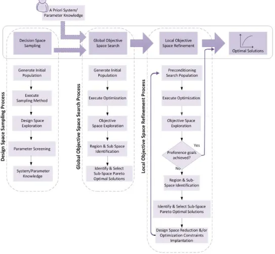
5.3 The SD-MOO Methodology for Supply Chain MOO ... 59
5.4 Conclusions ... 62
6. CASE1 – ACADEMIC CASE STUDY OF THE BEER GAME ... 63
6.1 Introduction to Chapter 6 ... 63
6.2 The Beer Game ... 63
6.3 Moo of The Beer Game ... 69
6.4 Results and Analysis ... 72
6.4.1 Analysis of The SD-MOO Methodology for Supply Chains ... 72
6.4.2 Scenario Analysis... 75
6.4.3 Scenario 1 vs Scenario 2 ... 79
6.4.4 Partitive Clustering Analysis ... 80
6.5 Conclusions ...89
7. CASE 2 – ACADEMIC CASE STUDY OF THE STOCK MANAGEMENT PROBLEM ... 91
7.1 Introduction to Chapter 7 ... 91
7.2 The Stock Management Problem ... 91
7.2.1 The Inventory Management Model... 95
7.3 MOO of The Inventory Management Model ... 97
7.4 Results and Analysis ... 99
7.4.1 Pareto Analysis ... 99
7.4.2 Higher Level Innovization on Inventory Management Problem ... 103
7.5 Conclusions ... 106
8. CASE STUDY 3 – AN INDUSTRIAL APPLICATION STUDY ... 107
8.1 Introduction to Chapter 8 ... 107
8.2 System Description ... 108
8.3 The System Dynamics Model and its Modules ... 110
8.3.1 Customer Order Rate ... 111
8.3.2 Demand Forecasting ... 113
8.3.3 Master Production Schedule ... 114
8.3.4 Production Scheduling ... 116
8.3.5 Production ... 118
8.3.6 Replenishment and Dispatching ... 119
8.3.7 Order Fulfilment ... 123
8.3.8 Backlog ... 124
8.4 Simulation Settings ... 126
8.4.1 Numerical Integreation and Time Step... 126
8.4.2 Initial Conditions and Model Settings ... 128
8.5 Simulation Scenarios ... 129
8.5.1 Scenario 1 and Scenario 2 ... 130
8.5.2 Scenario 3 ... 131
8.5.3 Scenario 4 ... 131
8.5.4 Scenario 5 ... 132
8.5.5 Scenario 6 ... 133
8.5.6 Scenario 7 and Scenario 8 ... 134
8.5.7 Scenario 9 ... 136
8.6 Model Validation ... 137
8.7 MOO for The Case Study ... 139
IX
8.8.2 Innovization ... 144
8.9 Industrial Implications ... 152
8.9.1 Analysis of Design Variables and Optimization Objectives ... 152
8.9.2 Critical WIP Zones ... 157
8.10 Conclusions ... 160
9. CONCLUSIONS AND FUTURE WORK... 163
9.1 Introduction to Chapter 9 ... 163
9.2 Overall Conclusions ... 163
9.3 Contributions to Research and Knowledge ... 164
9.4 Future Work ... 168
9.4.1 Additional Experimentation ... 168
9.4.2 Taking Stochastics Into Account ... 168
9.4.3 Multi-Level-MOO For Supply Chains ... 169
10. REFERENCES ... 173
APPENDIX I: CASE 3 SIMULATION SCENARIOS ... 183
APPENDIX II: CASE 3 SCENARIO VARIABLE BOUNDRIES ... 193
XI
LIST O F FIG URES
Figure 1.1: Case studies incorporating the stock management problem. ... 4
Figure 1.2: A multi-methodological research approach . ... 6
Figure 1.3: A simple SD stock and flow model with feedback loop. ... 8
Figure 1.4: A general Simulation Based Optimization process. ... 12
Figure 1.5: Concept of Non-domination, Decision and Objective Space. ... 12
Figure 1.6: General Pareto-based MOO procedure. ... 13
Figure 1.7: A synoptic taxonomy of MOO approaches. ... 14
Figure 1.8: Post-optimal analysis process. ... 16
Figure 1.9: Relationship between major thesis chapters. ... 17
Figure 2.1: Modeling techniques and Mathematical approaches. ... 36
Figure 2.2: Research scope and Optimization techniques. ... 37
Figure 2.3: Optimization objectives. ... 38
Figure 3.1: Integrating Optimization and SD for running MOO. ... 40
Figure 3.2: The VensimInterface arguments. ... 40
Figure 3.3: A workflow in modeFrontier using the VensimInterface. ... 41
Figure 3.4: VensimInterface internal process. ... 42
Figure 4.1: A Parallel Coordinate plot. ... 46
Figure 4.2: Parallel Coordinate plot with filtering. ... 47
Figure 4.3: A overall taxonomy of Clustering approaches, (Xiao and Yu, 2012). ... 47
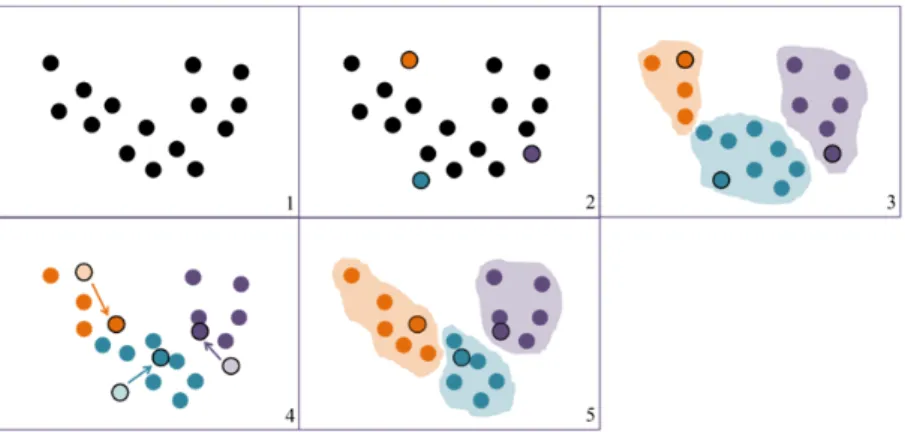
Figure 4.4: The k-mean algorithm process. ... 49
Figure 4.5: Pseudo code for inorder tree traversal. ... 50
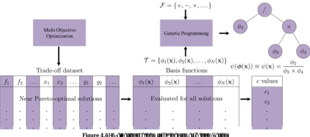
Figure 4.6: Evaluation of binary trees in automated innovization. ... 51
Figure 4.7: Grid-based clustering. ... 51
Figure 4.8: Higher Level Innovization with a parameter P. ... 54
Figure 5.1: Decision maker and optimization interaction combinations. ... 58
Figure 5.2: Methodology for SD-MOO. ... 60
Figure 6.1: A generic SD BG entity model. ... 64
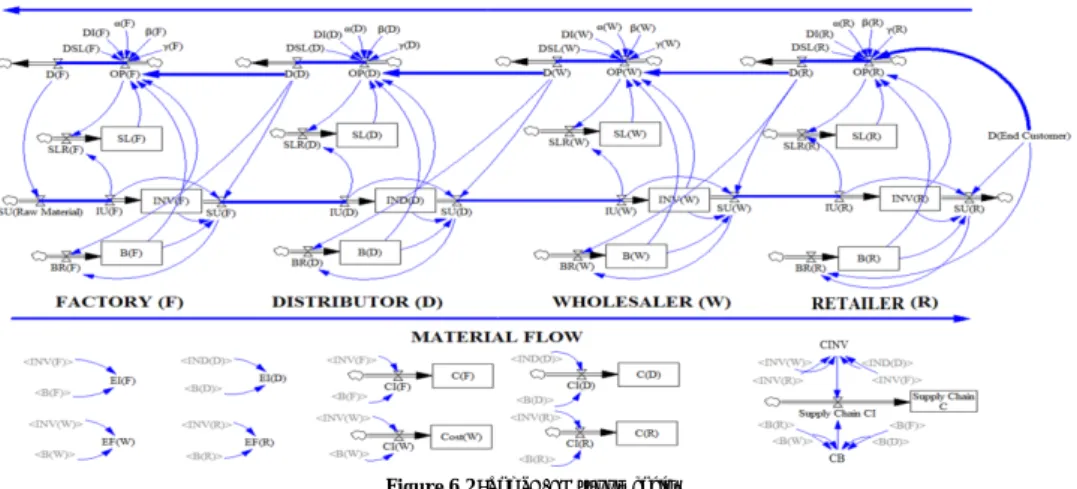
Figure 6.2: The SD-BG supply chain. ... 68
Figure 6.3: The bullwhip effect. ... 69
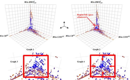
Figure 6.4: Pareto-optimal solutions for S2 obtained from global objective search. ... 72
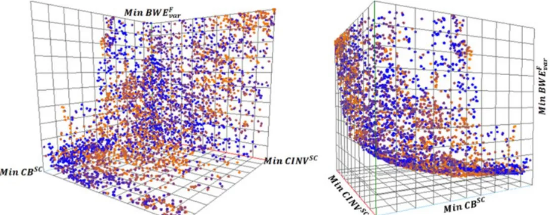
Figure 6.5: Final Pareto-optimal solutions for S2 obtained from local objective search... 73
Figure 6.6: Final Pareto-optimal solutions for S1 obtained from local objective search. .. 73
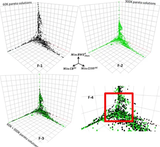
Figure 6.7: Comparison of 60K and 300K Pareto-optimal solutions. ... 74
Figure 6.8: Parallel Coordinate of S1 Pareto Solutions. ... 75
Figure 6.9: Parallel Coordinate of S2 Pareto Solutions. ... 77
Figure 6.10: S1 and S2 average values sorted on total supply chain cost. ... 79
Figure 6.13: PC plot of S2 clustered Pareto solutions. ... 82
Figure 6.12: PC plot of S1 clustered Pareto solutions. ... 82
Figure 6.14: Comparison of S1 and S2 clustered Pareto solutions. ... 85
Figure 6.15: Cost comparison of S1 and S2 clustered Pareto solutions. ... 86
Figure 6.17: Best solution in terms of CSC. ... 87
Figure 6.16: All Pareto-Optimal solutions in cluster S2-C2. ... 87
Figure 6.18: Comparing BG default run with the chosen Pareto solution (EV. 101209). .. 89
Figure 7.1: Generic stock management structure (Sterman, 2000). ... 93
Figure 7.2: The inventory management model, adopted from (Sterman, 2000). ... 96
Figure 7.3: Pareto-optimal solutions with a customer demand of 10000 products/week. ... 100
Figure 7.4: Pareto-optimal solutions with a customer demand of 15000 products/week. ... 100
Figure 7.5: Pareto-optimal solutions of both optimization scenarios. ... 100
Figure 7.6: Correlation between and . ... 100
Figure 7.8: PC heat map of design variable and objective functions for Pareto-optimal solutions with 50% higher demand. ... 101
Figure 7.7: PC heat map for of all design variable and objective functions for Pareto-optimal solutions with original demand. ... 101
Figure 7.9: Pareto-optimal trade-off between and . ... 102
Figure 7.10: Higher level innovization cluster plot of rule 2 and 3. ... 105
Figure 7.11: Higher level innovization cluster plot of rule 10... 105
Figure 8.1: System overview. ... 108
Figure 8.2: Product flow through the entire system under study. ... 109
Figure 8.3: Customer Demand. ... 110
Figure 8.4: Policy Structure Diagram of the investigated industrial system. ... 110
Figure 8.5: Excel Demand data access and the generic Customer Order Rate structure. 111
Figure 8.6: Customer Order Rate for PA. ... 112
Figure 8.7: Generic structure of Demand Forecasting. ... 113
Figure 8.8: Estimated Customer Order Rate and Customer Order Rate. ... 114
Figure 8.9: Generic structure of Master Production Schedule. ... 114
Figure 8.10: Master Production Schedule. ... 115
Figure 8.11: Generic structure of Production Scheduling. ... 116
Figure 8.12: Generic structure of Production. ... 118
Figure 8.13: Generic structure of Replenishment & Dispatching. ... 119
Figure 8.14: Pseudo-code for eq.( 8.21) and eq.( 8.22). ... 123
Figure 8.15: Generic structure of Order Fulfillment. ... 123
Figure 8.16: Generic structure of Backlog. ... 125
Figure 8.17: Time Step and approximation of solution. ... 127
Figure 8.18: Simulation model depicting scenario 1 (and 2), a pure push system. ... 130
Figure 8.19: Simulation model depicting scenario 3. ... 131
Figure 8.20: Simulation model depicting scenario 4. ... 132
Figure 8.21: Simulation model depicting scenario 5. ... 132
Figure 8.22: Simulation model depicting scenario 6. ... 134
Figure 8.23: Simulation model depicting scenario 7. ... 135
Figure 8.24: Simulation model depicting scenario 8. ... 135
Figure 8.25: Simulation model depicting scenario 9. ... 136
Figure 8.26: 2D scatter plot all scenarios. ... 143
Figure 8.27: Parallel Coordinates of all scenarios and Scenario 9 vs Scenario 1 and Scenario 8. ... 146
Figure 8.28: Individual Parallel Coordinates of all scenarios. ...147
XIII
Figure 8.32: Parallel Coordinate Heat Map of for scenario 9. ... 153
Figure 8.31: Parallel Coordinate Heat Map of for scenario 9. ... 153
Figure 8.34: Parallel Coordinate of Pareto optimal solutions with an order fill rate of 95-98% and 99-99.9985% ... 155
Figure 8.33: Parallel Coordinate of best , and trade-off solution for 14.6. ... 155
Figure 8.35: WIP regions, adopted from (Pound and Spearman, 2007). ... 157
Figure 8.37: Scatter Plot over the different WIP zones. ... 159
XV
LIST O F TABLES
Table 1.1: Comparison of differences between SD and DES, adopted from (Brito et al.,
2011; Tako and Robinson, 2010). ... 10
Table 2.1: List of papers and their contents. ... 32
Table 6.1: Design and Objective parameter boundaries for S2-C2. ... 84
Table 7.1: Various of stock management structure application domains (Sterman, 2000). ... 92
Table 7.2: Range of variation of design variables for both scenarios. ... 99
Table 7.3: Higher Level Innovization (HLI) rules and their significance values. ... 103
Table 8.1: Summary of simulation scenarios. ... 137
1
C H A P T E R 1
INTRODUCTION
1.1 INTRODUCTION TO CHAPTER 1
This chapter presents the industrial and academic motivations behind this research, fol-lowed by its aim and objectives. The utilized research methodology and the key enabling technologies, including supply-chain modeling, system dynamics simulation, simulation-based optimization and multi-objective optimization, are briefly introduced. Finally, an overview of the organization of the thesis is provided.
1.2 RESEA RCH MOTIVATIONS
In today’s highly competitive global marketplace, companies and organizations need to find new ways to avoid waste through the effective design and efficient operations of their sys-tems. In other words, using new methods and tools to optimize their systems is the key fac-tor to leverage their effectiveness and to retain competitiveness. Computer simulation has been described as the most effective tool for designing and analyzing systems (De Vin et al., 2004). However, it is very often misunderstood in industry that simulation, if used stand-alone, is not a real optimization tool. Research efforts have been focused on integrating generative tools with simulation software so that “optimal” or close to optimal solutions can be found automatically. An optimal solution here means the setting of a set of control-lable design variables (also known as decision variables) that can minimize or maximize some measures of system performance.
The complex networks of supply chains are composed of several actors that strive toward different purposes and have multiple performance measures at different levels, which in most cases are in conflict with each other, which have to be taken into account in their op-erations. Due to the multiple performance measures, supply chain decision making is much more complex than treating it as a single objective optimization problem. When a supply chain is examined more closely, it is clear to see that it is a complex system that consists of multiple entities, e.g., suppliers, manufacturers, distributors, and retailers, as mentioned earlier, which individually have their own performance measures and objectives to opti-mize. While the retailer might aim to minimize the product price and lead time, the
dis-tributor might be measured upon its ability to fully utilize the warehouse and the stock-keeping-units (SKUs), as well as the responsiveness in consolidating the customer order by having short picking times or efficient picking routes. The manufacturer and supplier, on the other hand, have another set of key performance measures – while the manufacturer focuses on maximizing the throughput, minimizing the work-in-process together with imizing its production batch sizes and set-up times, the supplier might mainly seek to min-imize the work-in-process (WIP) and delivery time, as well as maxmin-imize quality and service levels. However, optimizing these individual entities is not adequate when optimizing a supply chain, as it is a dynamic network, consisting of multiple transaction points with complex transportations, information and financial transactions between entities. Hence, optimizing the supply chain as a whole is as crucial as optimizing the individual entities. Moreover, the aim of supply chain management (SCM) is to align and combine all these objectives, individual as well as the entire supply chain, so that they work towards a com-mon goal – increasing the efficiency and profitability of the overall supply chain. SCM is thus multi-objective in nature and involves several conflicting objectives, both at the indi-vidual entity level and at the supply chain level.
In general, optimization modeling approaches using, e.g., mathematical programming, re-quire equation-based models of the system under study. The models also rere-quire a com-prehensive knowledge of optimization from the developers and most real-world problems are too complex to be formulated as manageable mathematical equations (Hong, 2005). As a matter of fact, pure optimization models, when used on their own, are incapable of incor-porating the dynamic behavior and complexities of systems or processes such as supply chains (Better et al., 2008). Hence, in a supply chain optimization problem, the supply chain needs to be depicted through simulation modeling, in order to capture its dynamic behavior, and to be combined with optimization methods to attain optimal solution sets. Such a combined use of the two approaches is called simulation-based optimization (SBO). The simulation methodology used for the SBO framework is based on system dynamics, which is an approach built on information feedbacks and delays in the model, in order to understand the dynamical behavior a system (Angerhofer and Angelides, 2000). A system dynamics model facilitates the representation, both graphically and mathematically, of the interactions governing the dynamic behavior of the studied system or process, as well as the analysis of the interactions and their emergent effects. Modeling with system dynamics enables users to take a causal view of reality and implement quantitative means to investi-gate the behavior of the system and its response to various policies (Sterman, 2000). Hedenstierna (2010) points out that system dynamics has been instrumental in under-standing supply chain behavior which started with Forrester (1961), who proved the exist-ence of the bullwhip effect and, in relation to this, the detrimental effect of promotions on supply chain performance. Hedenstierna (2010) also explains that due to the system dy-namics’ tendency to consider several different types of flow networks, there is often a need for multi-objective approaches. Actually, such an idea can be found in much earlier publi-cations by researchers such as Gottschalk (1986) and Towill and Del Vecchio (1994). They discussed the use of multi-criteria utility functions. It is only recently that the research community has initiated experimentation with multi-objective optimization in combination with system dynamics models, such as Duggan (2008), Aslam et al. (2011) and Dudas et al. (2011). A comprehensive literature survey, presented in Chapter 2, shows that most of the research conducted on multi-objective optimization for SCM is based on mathematical ap-proaches, e.g., linear programming, mixed integer programming, mixed integer linear pro-gramming, etc. In comparison with the large amount of publications on applying simula-tion approaches to SCM problems, it seems that the explorasimula-tion of using simulasimula-tion-based optimization, especially within the context of multi-objective optimization, is far from ade-quate.
3 Generally speaking, a multi-objective optimization procedure generates a solution set in the objective space in which some of the solutions are optimal trade-off solutions among the optimization objectives. These optimal solutions are generally known as Pareto-optimal solutions which together constitute the so-called Pareto front. Thus, the generation of mul-tiple Pareto-optimal solutions through the multi-objective optimization procedure is better able to support a decision maker than a single-objective optimization, as the decision mak-er is provided with sevmak-eral optimal solutions to choose from when making a decision (Ng et al., 2012). However, as suggested by Ng et al. (2012), a subsequent question that can be more crucial to the decision maker is, ‘What makes these solutions optimal?’. According to Deb (2003), there should be some similar characteristics among the Pareto-optimal solu-tions which constitute their optimality. Bandaru and Deb (2013) also point out that acquir-ing the correlation between the design and optimization objectives in a sacquir-ingle problem can provide hidden knowledge for solving similar problems. For example, retrieving hidden knowledge from a specific problem might reveal that the Pareto-optimal solutions require a
design variable x to take a fixed or almost fixed value, whereas design variable y and
varia-ble z are required to be changed linearly or exponentially for an expected change in the
op-timization objectives. Hence, the insight acquired from such complex relationships not only provides useful knowledge about how to solve the problem at hand optimally, but also pro-vides can act as a rule of thumb for similar problems in the future. Such an idea of
knowledge extraction or discovery, through post-optimality analysis on the Pareto-optimal
solutions generated from multi-objective optimization, was first introduced by Deb and
Srinivasan (2006) in which they coined the term innovization, which means the act of
re-vealing innovation through optimization.
While the original innovization concept targeted engineering design problems, through a number of industrial application case studies, it has been shown to be an equally powerful method for systems analysis and decision support for production systems (Dudas et al., 2013, 2011; Ng et al., 2013, 2011). In particular, Dudas et al. (2013) introduce a distance-based simulation-distance-based innovization (SBI) method that specifically aims to tackle the sto-chastic simulation output data. In comparison to the original innovization procedures re-ported in Deb and Srinivasan (2006), as well as the recently developed automated inno-vization algorithms revealed in Bandaru and Deb (2013b, 2011), which perform post-optimality analysis only on the Pareto-optimal solution sets, the uniqueness of the dis-tance-based SBI methodology is that it uses the entire dataset generated from multi-objective optimization, so that it is possible to distinguish what characteristics the ‘bad’ (non-optimal) solutions possess. On the other hand, while the successful applications of innovization have been illustrated in these recent studies for production systems analysis, applying the innovization concept to any supply-chain systems has, to our best knowledge, never been reported. Additionally, while discrete-event simulation (DES), commonly used for production systems simulation, can be effectively used for supply-chain system simula-tion to a certain scale, when the number of entities involved are many and the simulasimula-tion time horizon is long (not uncommon to simulate the behavior of a supply chain for more than 1 year), DES can be an ineffective approach for studying SCM under a SBO frame-work. Consequently, there is a need to develop a new SCM analysis method that links SBO, in particular multi-objective optimization, to system dynamics models, which also covers the post-optimality analysis step. It is strongly believed that such a novel SD-SBO-innovization methodology can be used to gain new insights for general SCM analysis, as well as to provide useful knowledge to support specific but practical decision making in in-dustry. Such knowledge cannot be obtained by any other existing approaches and therefore represents the prime impetus of this research study. A comprehensive discussion regarding DES and SD can also be found in Section 1.6.
However, a SD-SBO-innovization methodology will require addressing the issue of manag-ing the so-called curse of dimensionality, which refers to the issue of a significant increase in combinatorial difficulty as the number of variables, such as input and output parame-ters, or dimensions, that is, optimization objectives, increases (Kuo and Sloan, 2005). Ob-taining optimal solutions for a MOO problem is generally far more time-consuming than finding optimal solutions for a single-objective optimization problem. The latter requires less computation time due to the fact that the optimization only needs to search in one di-mension (Chen et al., 2002). Deb and Saxena (2005) point out that increasing the dimen-sionality of the objective space, i.e., implementing multiple objectives, will also increase the dimensionality of the Pareto front, resulting in an exponential increase in the number of points required to represent the Pareto front. In addition, high dimensionality of input and output variables, i.e., large amount of input and output parameters, will generate an expo-nential growth in difficulty regarding the modeling of the problem and optimization (Shan and Wang0, 2010). Also, due to the combinatorial explosion of the problem, both the effi-ciency and accuracy of the optimization are also sacrificed (Koch et al., 1997).
The SD-SBO-innovization methodology is evaluated through three case studies, in which case study 1 and 2 are based on well-known academic supply chain problems, whereas case study 3 presents a MOO of a real-world internal supply chain. All three case studies incor-porate the so-called stock management problem, as shown in Figure 1.1, which refers to the issue of optimally regulating a stock or system to meet some system objectives, such as managers seeking to attain low inventory levels whilst providing 100% service levels in terms of fulfilled orders.
Figure 1.1: Case studies incorporating the stock management problem.
Case study 1 is based on the Beer Game, originally developed at the MIT Sloan School of Management in the 1960´s (Sterman, 1989), which replicates a four echelon supply chain mimicking beer production and distribution with the overall objective of fulfilling customer demand whilst minimizing the inventory and backlog levels. The game also demonstrates the existence of the so-called bullwhip effect. In case study 2, MOO and post-optimal analy-sis is performed on the inventory management model that represents a structure of a single supply chain entity which seeks to find the optimal trade-offs between the sufficient supply line, inventory coverage and customer demand. Sterman, (2006) points out that in order to understand the behavior of a supply chain as well as the cause of its instability, it is neces-sary to study and understand the structure and dynamics of a single entity by exploring how the single entity balances its production and inventory levels in order to fulfill custom-er demand. On the othcustom-er hand, case study 3 is based on a real-world application depicting an internal supply chain of a manufacturing company that seeks to balance system WIP levels whilst decreasing the delivery delay to customer as well as evaluating different de-grees of push and pull production strategies.
5
1.3 RESEA RCH AI M AND OBJECTIVES
The aim of this thesis is to address the supply chain optimization problem within a truly Pareto-based multi-objective context and utilize knowledge extraction techniques to extract valuable and useful information from the Pareto-optimal solutions. Knowledge extraction means detecting hidden interrelationships between the Pareto solutions, identifying com-mon properties and characteristics of the Pareto solutions, as well as discovering concealed structures in the Pareto-optimal dataset, in order to support managers in their decision making. This research aim can be further refined into the following objectives:
1. Develop and implement an application interface for integrating SD and MOO
software, in order to realize the SD-SBO-innovization methodology and apply it to subsequent application studies.
2. Explore and apply data analysis methods and knowledge extraction techniques on
the Pareto-optimal datasets to assist decision makers to obtain knowledge about the problems before they make their choices.
3. To introduce a method for supply chain multi-objective optimization using System
Dynamics that can be able to specifically cope with the problem of high dimen-sionality or so-called curse of dimendimen-sionality, so that optimization data can be generated within a reasonable time.
4. Evaluate the proposed integrated applications and methodology against two
aca-demic test cases as well as a real industrial application study.
1.4 RESEA RCH ME THODO LOGY
In addressing the research questions, a multi-method approach is adopted that combines
quantitative and qualitative research. Robson (2011) explains that quantitative research
makes use of numerical data and seeks to identify findings that can be generalized to the
world at large. In contrast, qualitative research is typically non-numerical and concerned
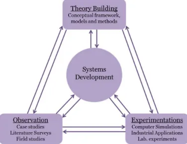
with an in-depth understanding of phenomena within specific contexts. According to John-son et al. ( 2007), combining quantitative and qualitative research into multi-method strat-egies often provides a greater understanding of the phenomena being studied and increases confidence in the generated results. The overall methodical framework of this thesis is based on the multi-methodical approach proposed by Nunamaker et al. (1990) which
con-sists of four main building blocks, namely observation, theory building, experimentation
and system development. Following the research approach as shown in Figure 1.2, a
com-prehensive study (observation) regarding the existing supply chain MOO approaches is conducted in the early phases of this work. The outcome of this study subsequently gener-ated new ideas and concepts (theory building). Nunamaker et al. (1990) point out that the theory building activity is the seedbed from which research objectives and hypothesis may emerge as well as assist in guiding the design of experiments and conduct systematic
ob-servations. Hence, the theory building activity has revealed the necessity of developing the SD-MOO interface and SD-MOO supply chain methodology as well as guided the selection of suitable case studies. The experimentation activity bridges the gap between theory build-ing and observations as it concerns itself with validatbuild-ing the underlybuild-ing theories through the cases studies (Nunamaker et al., 1990). On the other hand, system development im-plements new and/or utilizes existing technological tools and applications in order to test, measure and validate the underlying theories and concepts to demonstrate their feasibility and applicability, which for the current research has been executed through the develop-ment and impledevelop-mentation of the SD-MOO interface.
Figure 1.2: A multi-methodological research approach .
An overview of the specific methods adopted in this study is presented below for the re-spective research objective.
Objective 1: Develop and implement an application interface for integrating SD and MOO software in order to realize the SD-SBO-innovization methodology and apply it to subse-quent application studies.
This objective is addressed using two research methods: literature review and software
development. A literature review of existing, related research is first conducted to establish a deep understanding of the research area and explore requirements for integrating Sys-tems Dynamics and Multi-Objective Optimization. Through software development, a sys-tem that connects Syssys-tems Dynamics and Multi-Objective Optimization within an SBO framework is then designed and implemented. The use of software development as a re-search method is described, amongst others, in (Nunamaker et al., 1990) and (Hasan, 2003).
O2: Explore and apply data analysis methods and knowledge extraction techniques to the Pareto-optimal dataset to assist decision makers to obtain knowledge about the problem before they make their choices.
The methods applied to address this objective are experiments and statistical analysis.
7 quantitative data. The collected datasets are then processed and analyzed using statistical
methods to draw conclusions.
O3: To introduce a method for supply chain multi-objective optimization using System Dynamics that can be able to specifically cope with the problem of high dimensionality or so-called curse of dimensionality, so that optimization data can be generated within a reasonable time.
This objective is addressed using two methods: literature review and constructive
re-search. A literature review of existing strategies for tackling the curse of dimensionality in a multi-objective context is first conducted, in order to identify the strengths and weakness of existing solutions. The findings from the analysis are then used to construct a new meth-odology for supply chain multi-objective optimization. The method of constructive research is discussed, for example, by Shaw (2001) and Koskinen et al. (2012).
O4: Evaluate the proposed integrated applications and methodology against two aca-demic test cases as well as a real industrial application study.
To address this objective, application case studies are conducted. The use of case studies as a research method allows for contextual conditions to be covered and for contemporary events to be examined (Yin, 2003). First, two application case studies are performed on well-known academic problems to enable the results to be benchmarked and replicated. A third application case study is then performed on a real-world problem to evaluate the in-dustrial relevance of the proposed methods and techniques.
1.5 SUPPLY CHAIN MODELI NG
Modeling is an effective way of designing, understanding, or analyzing real-world processes and systems. A model enables a decision maker to gain a better understanding of the com-plexity of a process/system and evaluate/predict its performance under various circum-stances. A supply chain incorporates the integrated processes where products are trans-formed from raw material, e.g., from the suppliers, to finished products delivered to end customers. Typically, these processes include different business functions in a company, e.g., procurement, production, logistics, etc., the need to collaborate, coordinate and inter-act with each other, in order to produce the commodity of the supply chain (Kim et al., 2004). Hence, supply chains can be seen as good examples of such complex systems which require the modeling of processes in the presence of multiple autonomous entities (i.e. suppliers, manufacturers, distributors, retailers, etc.), multiple performance measures and multiple objectives, both local and global, which together constitute very complex interac-tion effects (Keramati, 2010). Li et al. (2002) describe that supply chain modeling is more or less a prerequisite for supply chain integration and present four incentives for supply chain modeling: (1) capturing supply chain complexities, e.g., interaction effects between supply chain members, by better understanding and uniform representation of the supply chain; (2) designing the supply chain management process in order to manage supply chain interdependencies; (3) establishing the visions to be shared by supply chain members and provide the basis for supply chain coordination and integration; and (4) facilitating the re-duction of supply chain dynamics at supply chain design phases. Over the years, supply chains have been depicted with many different modeling approaches, ranging from process models, statistical models, optimization models, analytical models as well as simulation
models. Simulation models in turn can be developed using various simulation techniques, such as agent-based modeling, discrete event modeling, and system dynamics modeling. A comprehensive taxonomy of various modeling approaches used over the years is presented in Keramati (2010). A more comprehensive review regarding the different modeling ap-proaches for supply chains can be found in Beamon (1998); Hung et al., (2006); Vidal and Goetschalckx (1997).
1.6 SYSTEM DYNAMICS
The modeling method for supply chains proposed in this work is based on system dynamics (SD), which is an approach built on information feedbacks and delays in the model, in or-der to unor-derstand the dynamical behavior of a system (Angerhofer and Angelides, 2000). A SD model facilitates the representation, both graphically and mathematically, of the inter-actions governing the dynamic behavior of the studied system or process, as well as the analysis of the interactions and their emergent effects. Modeling with SD enables users to take a causal view of reality and implements quantitative means to investigate the behavior of the system and its response to various policies. According to Campuzano and Mula (2011), SD is a rigorous approach to qualitatively describe and explore supply chain pro-cesses, information, strategies, and organizational limits. It also facilitates modeling, exper-imentation and the analysis of both qualitative and quantitative aspects of supply chain de-sign and the management of the supply chain and its network, without requiring compre-hensive information or precise data, because it emphasizes the dynamic performance of the investigated system through the combination of feedback loops. A SD model is derived from the internal nonlinear structure of the system and is able to create new kinds of be-haviors that might not have been observed in the present time but may occur in the future (Bhushi and Javalagi, 2004). Sterman (2000) describes a supply chain as a system contain-ing multiple autonomous entitles, which is characterized by a stock and flow structure for acquisition, storage, converting inputs into outputs, as well as the decision rules governing these flows. The existing flows in the supply chains, such as information, material, orders, money, etc., create important feedbacks among the members of the supply chain, thus making SD a well-suited approach for modeling and analyzing supply chains (Georgiadis et al., 2005). SD is based on three central building blocks, namely; stocks, flows, and feed-backs, where stocks are accumulations which depict the state of the system and the content of the stock is only changed through its in-and outflow. The flows, on the other hand, are controlled through the ratio of various model variables that change the flows and thus the stocks. The feedback loops represent the corrective measures taken by the system or a deci-sion maker, in order to adjust the value of a variable towards its actual value or a desired value (Campuzano and Mula, 2011).
Figure 1.3: A simple SD stock and flow model with feedback loop.
Inventory
Production Rate
Shipment Rate
Production Start
Rate
Inventory Gap
Desired Inventory
+
+
-+
B
Feedback loop9 Figure 1.3 depicts a SD stock and flow model representing a simple manufacturing process, utilizing the three building blocks of system dynamics modeling. In the manufacturing pro-cess depicted in Figure 1.3, it can be seen that the stock in this propro-cess is represented by the system’s inventory where the inflow of production and the outflow of shipment rates in-crease and dein-crease the accumulated inventory levels. The production rate and inventory gap variable constitutes the flow of products into the inventory, by defining the ratio pro-duction rate variable. The inventory gap variable is part of the feedback loop which takes corrective measures to keep the inventory at a desired inventory level, by increasing or de-creasing the inventory gap. As explained, the stocks accumulate or integrate their flows where the net flow or rate, i.e., the inflow less the outflow, into the stock is the rate by which the stock is changed, and where the stock, in this case the inventory, corresponds to
the following integral equation, where production rate(s) represents the inflow to the
in-ventory at a time s between the initial time and current time :
(1.1) However, in this work the process of accumulation of a stock is represented as:
(1.2)
Where represents the inventory in the previous time period, and ,
, represent the variable values at current time . For a
more comprehensive introduction to system dynamics modeling, implementation, and analysis, the reader is referred to Forrester (1961), Sterman, (2000) and Morecroft (2007).
1 . 6 . 1 S Y S TE M D Y N A M I CS A N D D I S C R E T E E V E NT S I M U L A
-T I O N
Another frequently utilized modeling, experimentation, and analysis tool for decision sup-port of logistics and supply chain problems is discrete-event simulation (DES). The two modeling methods, i.e., SD and DES, are quite different in their approaches. DES models a system as a network of queues and activities, and where the system state is changed at a discrete point of time, whereas SD models, as explained, are based on stocks and flows in which the system state is continuously changing (Brailsford and Hilton, 2001). Tako and Robinson (2009) explain that in DES each entity, i.e., products, is individually represented where specific attributes are attached to these entities in order to follow and determine what happens to them during the simulation. On the other hand, in SD, entities are repre-sented in a continuous quantity, like a fluid passing through a tank, making it impossible to follow individual entities. A comparison of various differences between SD and DES is pre-sented in Table 1.1.
Aspects DES SD Modeling
perspective
Analytical, emphasis on detail complexity
Holistic, emphasis on dynamic complexity
Problem Scope Operation/Tactical Strategic
Randomness Utilizes random variables through
statistical distributions Stochastic features are less often utilized, averages of
vari-ables are used instead
Building Blocks Network of queues and activities Series of stocks and flows
Resolution Individual entities, attributes,
decision and events Homogenized entities, continu-ous policy pressure
State Change At discrete point of time, where the model state is updated at en event-step
Continuous, where the model state is updated at very small time step
Data Quantitative Quantitative and Qualitative
Feedback
effects Models open loop structures, less interested in feedbacks Models casual relationships and feedback effects
Model Results Provides statistically valid
esti-mates of system performance. Provides a full picture, both quantitatively and qualitatively,
of the system performance
Table 1.1: Comparison of differences between SD and DES, adopted from (Brito et al., 2011; Tako and Robinson, 2010).
Morecroft (2007) argues that the differences do not only lie within the technical character-istics of the two approaches, i.e., queues versus stocks, discrete versus continuous, stochas-tic versus determinisstochas-tic, but also in their worldview. In accordance with this aspect, SD
deals with a deterministic complexity and DES with a stochastic complexity. While the
dy-namic behavior in SD is based on the feedback structure in the model, in a DES model the dynamic behavior arises from the interactions between the random processes. According to Morecroft (2007), this suggests that the unfolded future in a SD model is partly and cantly predetermined, whereas in a DES model the unfolded future is partly and signifi-cantly a matter of chance. While a problem from a SD worldview is investigated by first identifying the feedback loops as well as the essential stocks, policies and information flows of the system and then redesigning these policies in order to change the feedback struc-tures and improve system performance, in the DES worldview the problem is addressed by first identifying connecting random processes, together with their underlying probabilities, queues, and activities, and then identifying more appropriate ways of handling the stochas-tic nature of the system, in order to improve system performance (Morecroft, 2007). More-croft (2007), together with several other researchers such as (Brailsford and Hilton, 2001; Brito et al., 2011; Lane, 2000), point out that DES is more suitable for operational and tac-tical level problems, since DES is able to handle operational detail as well as stochastic pro-cesses which are suitable for portraying details within operations, such as a process of products moving through a set of interacting stochastic machines in a production line. In addition, as random processes release individual entities, such as a product into a succes-sive machine, DES is able to represent the details of the movements and queues of these individual products in the production line. In other words, the attention to details is an es-sential characteristic 0f DES modeling. SD models, on the other hand, according to the above-mentioned authors, are more suitable for handling strategic level issues with their aggregated stock accumulation, flows, and coordinating network of feedback loops. More-croft (2007) explains that in contrast to DES, a SD model would provide a distance view of the operations in a production line where, instead of portraying machines, conveyers, buff-ers etc., the SD model would portray inventory, workforce, pressure-driven policies for in-ventory management and control, as well as workforce hiring. Furthermore, due to the ho-listic view of the production line operations, a SD model is able to depict feedback loops that embrace the different functions and departments of the depicted system. However,
11 despite the differences between the two approaches, Sweetser (1999) points out that the main objective of both simulation approaches is to understand the behaviors of a modeled system over time, as well as to compare the system’s performance when subjected to vari-ous conditions. According to Morecroft (2007), the selection between these approaches de-pends on the scope of the problem, the scale and level of detail required, as well as the modeler’s preference. For a comprehensive discussion regarding the differences and simi-larities between DES and SD, as well as their suitability regarding problem scope, i.e., stra-tegic, tactical or operational, the reader is referred to Brailsford and Hilton (2001); Brito et al., (2011); Lane (2000); Tako and Robinson (2012, 2010). As previously explained, SD is the modeling approach utilized in this work because all the case studies conducted are more suitable to be depicted through SD than DES. Case 1 and 2 are well-known studies within the SD domain which deals with dynamic decision making and complexity. Howev-er, these studies have so far, to our knowledge, never been studied from a SD-SBO perspec-tive. On the other hand, application case study 3 requires a more holistic perspective of the studied system in order to provide a complete picture, both qualitatively and quantitatively, of the system performance. Additionally, as explained before, the computation time for an evaluation is significantly lower for a SD model then for a DES model of equivalent level of abstraction, making SD a more preferable choice from a SBO point of view.
1.7 SIMULATION-BASED OPTIMIZATION
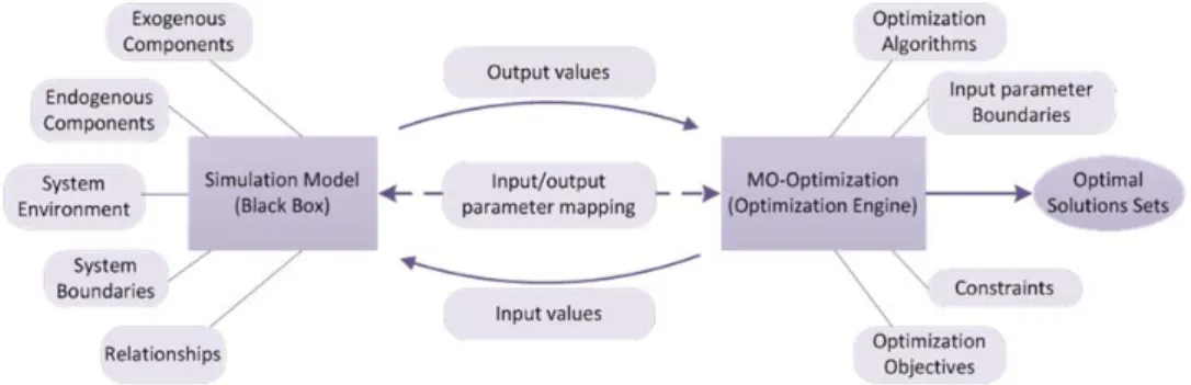
SBO is the process of obtaining optimal system settings from sets of decision variables, i.e., input parameters, where the objective functions and performance of the system are evalu-ated through the output results of the simulation model over the system (Ólafsson and Kim, 2002). Figure 1.4 presents a generic SBO process in which the optimization problem and the simulation model are defined separately. The optimization engine incorporates the optimization algorithms, input parameter boundaries, constraints, and the optimization objectives, while the simulation model includes the depiction of the system environment, its boundaries, as well as the endogenous and exogenous components and their relation-ship within the system. The two modules are connected through the defined input and out-put parameters, where the parameters are mapped into respective module. SBO is an itera-tive process which is initiated through the optimization algorithm by generating a set of values for the decision variables within the parameter boundaries. These values then act as input values for the simulation model. After receiving the input values from the optimiza-tion engine, the simulaoptimiza-tion run is executed, thus computing the performance measures of the system. The performance measures, which include the optimization objectives and oth-er output parametoth-ers of intoth-erest, are then fed back to the optimization engine. Based on this feedback of current and past evaluations, the optimization algorithm then generates a new set of decision variables for evaluation. This process is iterated until a stopping criteri-on is fulfilled, which might be that a certain amount of time has passed, objective values have been reached, a defined number of evaluations have been performed, etc., (Syberfeldt, 2009). Hence, the SBO process treats the simulation module as a black box into which the optimization engine feeds input values and from which it receives the response generated by the simulation. Syberfeldt (2009) identifies several advantages of separating simulation and optimization into individual modules. One of the main advantages is the possibility to alter or develop the simulation model, without having to alter the optimization algorithm and the opportunity to exploit the optimization algorithm in other problem areas or do-mains.
Figure 1.4: A general Simulation Based Optimization process.
1.8 MULTI- OBJECTIVE OPTIMIZATION
Multi-objective optimization (MOO) is a discipline that has been studied since the 1970s. Its application areas range widely from resource allocation, transportation, and investment decisions to mechanical engineering, chemical engineering, and automation applications, to name a few. In contrast to single-objective optimization, in which only one objective function is considered, MOO considers multiple objective functions simultaneously and
seeks to identify a set of optimal solutions which are defined as Pareto-optimal solutions.
A
solution is considered to belong to the Pareto-optimal set when there is no other solution that can improve at least one of the optimization objectives without deteriorating any other objective. This set of solutions is also known as the Pareto front when plotted on the objec-tive space. Figure 1.5 illustrates the concept of decision and objecobjec-tive space, as well as the domination and non-domination of solutions in MOO. The search space of a multi-objective optimization problem is represented by the decision space where the design vari-ables, i.e., the input parameters, constitute a set of solutions that are evaluated through a solver, which in this work is mainly a simulation model, and mapped to the objective space.
Thus, a certain solution A with its inherent values of the design parameters x and x is
evaluated through the solver which subsequently results in A′ in the objective space
repre-senting the fitness or performance of solution A in terms of the objective functions f and f .
13 The main concept of MOO is to evaluate two or more conflicting objectives against each other and obtain the Pareto-optimal solutions and the Pareto front (Basseur et al., 2006). This comparison of the solutions is executed on the basis of the domination concept in
which a solution is said to dominate a solution if is no worse then , with respect to
all optimization objectives, and where is strictly better than in at least one optimiza-tion objective (Deb, 2001). A simple method of handling a MOO problem is to form a com-posite objective function as the weighted sum of the conflicting objectives. Since the weight for an objective is proportional to the preference factor assigned to that specific objective,
this method is also called the preference-based strategy (Deb, 2001). Apparently,
prefer-ence-based MOO is simple to apply, because by scalarizing an objective vector into a single composite objective function (e.g., combining all performance measures into a weighted average objective function to represent the overall system cost), a MOO problem can be converted into a single-objective optimization problem and, thus, a single trade-off optimal solution can be sought effectively. However, the major drawback is that the trade-off solu-tion obtained by using this procedure is very sensitive to the relative preference vector. Therefore, the choice of the preference weights and thus the obtained trade-off solution is highly subjective to the particular decision maker. At the same time, it is also argued that using preference-based MOO to obtain a single ‘‘global’’ optimal solution for multi-tier sys-tems, like supply chains, is not desirable if the ‘‘global’’ optimum suggests a set of decision variable values that may sacrifice the performance of the sub-system level. For example, the optimal solution found by the simulation optimization may be optimal when the overall supply chain is considered, but totally unacceptable to the company that plays the role of the manufacturer. Therefore, for a decision maker, it would be useful if the posterior Pareto front can be generated quickly by using a MOO algorithm, as shown in Figure 1.6, so that he/she can choose the most suitable configuration among the trade-off solutions generated.
Figure 1.6: General Pareto-based MOO procedure.
1 . 8 . 1 M U L T I - O B J E C T I V E M E T A - H E U R I S T I CS
As in the case of single-objective optimization, MOO approaches can be classified into
ex-act algorithms and approximate algorithms which are also known as heuristic approach-es. Basseur et al. (2006) point out that exact search algorithms are more suitable and effec-tive for small size problems and problems with up to two optimization objeceffec-tives, as not
many exact approaches can cope with the issues of the problem’s NP-hardness complexity and the multi-objective nature of the problem at once.
Figure 1.7: A synoptic taxonomy of MOO approaches.
Heuristic approaches, on the other hand, are essential for solving large-size problems, such as NP-hard problems and problems with two or more optimization objectives. However, heuristic methods cannot be guaranteed to find the exact optimal sets, instead, these ap-proaches obtain an approximation of the optimal set as they seek to obtain feasible/near-optimal solutions at a reasonable computational cost (Basseur et al., 2006). Heuristic
ap-proaches are further divided into specific heuristics and meta-heuristics, as shown in
Fig-ure 1.7. Specific heuristic algorithms are specifically designed and developed for a certain problem. Meta-heuristics, on the other hand, are general purpose algorithms which are considered to be high-level strategies guiding underlying heuristic algorithms to explore the search space and solve the optimization problem (Blum and Roli, 2003). Jones et al.
(2002)argue that the greatest advantage of meta-heuristic algorithms, besides the fact that
they are well-suited to optimizing NP-hard problems, as in the case of heuristic algorithms in general, is their flexibility regarding their applicability to a diverse set of problem do-mains and optimization problems. This is mainly due to the fact that the optimization func-tion is considered as a black-box, and their connectivity to a range of modeling approaches. Over the years, researchers have also demonstrated the applicability of meta-heuristics to supply chain problems. For example, in their state-of-the-art review regarding SBO
ap-proaches in the context of SCM, Abo-Hamad and Arisha (2011) disclose that
meta-heuristics has been the most popular and implemented optimization technique during the last decade, within the application areas of SCM, such as inventory management, produc-tion planning & scheduling, transportaproduc-tion & logistics, as well as supply chain design, and integration & collaboration. A compressive review regarding the implementation of meta-heuristic algorithms in the supply chain domain can be found in Abo-Hamad and Arisha (2011) and Griffis et al., (2012). Ramalhinho-Lourenco (2001) points out that features of the meta-heuristic algorithms are well-suited to solving SCM problems. Besides the ability to solve very complex and hard combinatorial optimization problems, their modular nature and problem independence results in shorter development and updating time of the opti-mization problem, which is crucial for coping with the rapid changes in a supply chain and the resulting short decision window for a decision maker. The features of meta-heuristics and their proven applicability in supply chain problems have motivated using them for the
optimization procedure implemented in this thesis. Meta-heuristics can utilize either a
sin-gle solution based search or a population-based search. A population-based search, in
contrast to a single solution based search,generates a whole population of solutions for
evaluation, whereas the single solution based search approach only has the possibility to
manipulate and evaluate one solution at a time. Talbi (2009) also explains that population-based algorithms are explorative in nature, i.e., they permit a diverse exploration of the search space, whereas single solution-based algorithms are better suited to finding
solu-15 tions within a specific region of the search space. When optimizing multiple objectives, the population-based approach is often chosen, since multiple Pareto solutions can be captured in a single optimization run with this approach. As the optimization procedure in this the-sis aims at multi-objective Pareto optimizations, the population-based approach has also been chosen in this work.
Although meta-heuristic algorithms can offer many advantages, their application is, how-ever, not completely straightforward. Talbi (2009) denotes that when meta-heuristics are applied to a multi-objective problem, the designer of the meta-heuristic algorithm has to
consider the dynamic balance of intensification and diversification, where intensification
refers to the exploitation of the best solutions found by the algorithm and convergence to the optimal solution sets, while diversification refers to the exploration of the search space and distribution of the obtained solutions around the optimal set. Hence, intensification ensures the generation of the approximated or near-optimal solutions and diversification ensures a wider spread of the optimal solutions covering different areas of the objective space, in order to limit the loss of valuable information regarding the trade-offs of the con-flicting objectives. Another aspect to consider with meta-heuristics is that many real-world problems are NP-complete, and NP-complete problems are known to be associated with a high computational cost, since finding an optimal solution requires an extensive search (Syberfeldt, 2009). A problem can also be computationally expensive even though it is not NP-complete; real-world optimization problems generally involve an immense number of possible solutions, and hundreds or thousands of simulation evaluations are needed before an acceptable solution is found (Boesel et al., 2001). This holds true especially for multi-objective problems, where a significantly larger portion of the search space needs to be ex-plored to obtain a set of Pareto-optimal solutions (Streichert et al., 2005). Even with im-provements in computer processing speed, one single simulation may take a couple of minutes or hours of computing time. This potentially renders enormous amounts of opti-mization time and is an issue that must be considered when applying meta-heuristics in real-world scenarios.
1.9 POST-OPTIMALITY
As earlier discussed, the MOO procedure generates a set of Pareto-optimal solutions, which are superior to all dominated solutions in the objective space and inferior to other Pareto-optimal solutions in at least one objective, thus providing a decision maker with a whole set of optimal alternatives to choose from, for the investigated problem. However, selecting a solution for implementation can be a difficult task, because the Pareto-optimal solution set can be very large (Taboada and Coit, 2006; Ulrich, 2012), in terms of volume, and difficult to visualize, in terms of dimensionality. Post-optimal analysis, which Venkat et al. (2004)
define as “the study of a set of solutions obtained from an optimization problem”, is thus
essential in multi-objective decision making, since the decision maker is required to identi-fy a Pareto-optimal solution or a subset of preferred Pareto solutions from a very large Pa-reto set. Here, it could be argued that by limiting the generation of such a huge PaPa-reto set, this issue could be resolved. However, Venkat et al. (2004) emphasize that the reason for acquiring a high-volume Pareto-optimal set is to provide the decision maker with a diverse set of unbiased solutions. Thus, managing and visualizing volume and high-dimensional datasets are crucial for decision making. Figure 1.8 illustrates the post-optimal analysis process and the post-optimal analysis tools utilized in this work. As the figure de-picts, the post-optimality analysis is performed on a Pareto-optimal solution set obtained
from the MOO and the supply chain-MOO methodology. The main concept of post-optimal analysis is not only to plot the Pareto-front, but also to visualize and analyze the relations between design variables, output variables, and the optimization objectives, in order to find and discover both evident and hidden properties of the solution set and thus the system and its behavior. The post-optimal analysis can be executed utilizing several different tools. This thesis work utilizes three post-optimal analysis tools for the post-optimal analysis
pro-cess and to manage the large Pareto set generated for the case studies, namely, Parallel
Co-ordinates, Clustering and Innovization. These three post-optimal analysis tools also assist in retrieving hidden insight and knowledge from the inherent properties and characteris-tics of the Pareto-optimal solutions. The post-optimal analysis itself is an iterative process in which the analyst or the decision maker continuously shifts between the post-optimal analysis tools, in order to better visualize, analyze, and discover the properties of the solu-tion set. In the same manner, the interacsolu-tion between the post-optimal analysis process and the analyst or decision maker is also iterative, because a first insight or new knowledge discovery about the system, for example, by obtaining decision rules and mathematical de-sign principles or discovering solution characteristics and hidden structures, could gener-ate further analysis and visualization of the dataset using the same or another post-optimal analysis tool. Each post-optimal analysis tool utilized in this thesis has its own characteris-tics and advantages which will be presented and discussed in Chapter 4.
Figure 1.8: Post-optimal analysis process.
1.10 THESIS
ORGANI ZATION
After this introduction chapter, the rest of the thesis is organized as follows: Chapter 2 pro-vides a comprehensive literature review over MOO for SCM which propro-vides the incentive of conducting the research presented in this thesis. Chapter 3 presents the new interface ap-plication developed in this research which facilitates interaction between SD and MOO software’s within a SBO-framework in order to generate Pareto-optimal solutions. Chapter 4 furthers the details of the concept of post-optimality and the post-optimal analysis tools utilized in this thesis, which are parallel coordinates, clustering and automated innoviza-tion, in order to understand and gain insight to evident any hidden properties of Pareto-optimal solution sets. Chapter 5 presents the novel SD-MOO methodology for supply chain MOO which supports the MOO to obtain the Pareto-optimal set in a computationally effi-cient manner by managing the curse-of-dimensionality issue in high-dimensional MOO problems. Chapter 6, 7 and 8 present three different application case studies which apply the techniques and methods introduced in the previous chapters. Two academic case stud-ies are presented in Chapter 6 and 7. While chapter 6 explores the MOO of the well-known
17 Beer Game, Chapter 7 conducts a MOO for the stock management problem. Chapter 8, on the other hand, provides a MOO analysis of a real-world industrial application case study of an internal supply chain, where different strategies are compared for a real-world automo-tive manufacturer in Sweden. Figure 1.9 illustrates the relationship between all these major chapters in this thesis and how they relate to the research aim and objectives described in Section 1.3. Finally, overall conclusions, contributions to knowledge, and future work that can be extended from this thesis work can be found in Chapter 9.