COMMUNICATION CONSTRAINTS
Commande d’une flottille de robots sous-marines avec des
contraintes de communication
Lara Bri˜n´on Arranz
CNRS, Control Systems Department, GIPSA-lab,
NeCS INRIA-CNRS team-project, Responsable: Carlos Canudas de Wit
February-Jun 2008
ENSIEG - INPG
INRIA Rhˆone-Alpes
1 Abstract 4
2 Introduction 5
2.1 Project Context . . . 5
2.2 Review of State of the Art . . . 6
2.2.1 Models . . . 6
2.2.2 Formation Control . . . 7
2.2.3 Formation control with collision avoidance . . . 10
2.3 Source Seeking control . . . 10
3 General Control Scheme 11 4 Formation Control 13 4.1 Circle Formation . . . 13
4.1.1 Circle with centre in (0,0) . . . 13
4.1.2 Circle with random coordinates of the centre . . . 16
4.1.3 Circle with centre in (c1, c2) . . . 16
4.2 Uniform Distribution . . . 17
5 Variable Formation Control 19 5.1 Main Transformations . . . 19
5.2 Limitation of the previous schemes . . . 20
5.2.1 Transitory response . . . 20
5.2.2 Slow variations . . . 21
5.3 Control Redesign based on previous schemes . . . 23
5.3.1 Contraction Algorithm . . . 24
6 Gradient Search Method 26 7 Conclusions 29 7.1 Review of results . . . 29 7.2 Perspectives . . . 30 8 Review in French 31 8.1 Introduction . . . 31 8.1.1 Contexte de stage . . . 31
8.1.2 Etude de l’´etat de l’art . . . 31
8.2 M´ethodologie . . . 33
8.3 Contrˆole de la formation . . . 33
8.3.1 Formation du cercle . . . 33
8.3.2 Distribution uniforme . . . 34
8.4 Contrˆole des variations de la formation . . . 34
8.5 Recherche du gradient . . . 35 8.6 Conclusions . . . 36 9 Attached Document A 37 9.1 Operators . . . 37 9.2 Calculations developed . . . 37 9.2.1 Formation Control . . . 37
9.2.2 Uniform Distribution Control . . . 39
9.3 Contraction circle control . . . 40
9.4 Gradient Search Control law . . . 42
9.5 Program code . . . 44
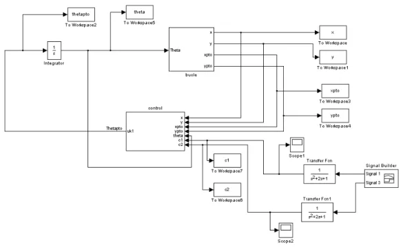
9.6 Simulink Diagrams . . . 55
10 Attached Document B: Review of the state of art 56 10.1 Introduction . . . 57
10.2 Models . . . 57
10.3 Formation Control . . . 59
10.3.1 Lyapunov-based control design . . . 59
10.3.2 Laplacian-based consensus algorithms . . . 62
10.3.3 Formation control with collision avoidance . . . 66
10.4 Source Seeking control . . . 68
10.4.1 Single agent with a single sensor . . . 68
1
Abstract
In this report we present the project Multi-agent control under communication constraints. The main objective is that a multi-agent system, composed of underwater vehicles which have to work in a cooperative way, find the position of a source (fresh water, chemical source,methane’s source). We show the simulation results and the mathematical development of the Lyapunov theorem for each problem.
Ce rapport pr´esente le stageCommande d’une flottille de robots sous-marines avec des con-traintes de communication. L’objectif trait´e est qu’une flottille d’agents sous-marins travaillent en collaboration, pour r´ealiser la recherche (par gradient) et la localisation d’une source (eaux douce, source chimique, source de m´ethane, etc.) On montre les r´esultats obtenus dans les sim-ulations et les calculs th´eoriques r´ealis´es en appliquant le th´eor`eme de Lyapunov.
2
Introduction
Control community had formerly focused mainly on control of vehicle formations. However, distributed motion and cooperation systems have emerged as topics of significant interest and matters of concern to the control theory and robotics specialists over the past few years.
This projectCommande d’une flottille de robots sous-marines avec des constraintes de com-munication tackles the problem of multi-agents control with communications constraints. The multi-agents system is composed of AUVs (Autonomous Underwater Vehicles). The aim of AUVs is to find the position of a source (fresh water, chemical source,methane’s source). In order to achieve this objective, the agents have to work in a cooperative way carrying out a gradient search through the concentration measurements of each agent.
2.1 Project Context
This work is included in the project CONNECT. It has been developed in five months but due to the complexity of this subject the thesis Control Design for Multi-Agent systems under communication constraints will continue with this research project.
Project CONNECT This project is funded by the ANR (National Research Agency). The project deals with the problem of controlling multi-agent systems, i.e. systems composed of several sub-systems interconnected between them by an heterogeneous communication network. The main challenge is to learn how to design controllers accounting for constraints on the net-work topology, but also on the possibility to share computational resources during the system operation, while preserving closed-loop system stability. The control of an agents cluster com-posed of autonomous underwater vehicles, marine surface vessels, and possibly aerial drones will be used as a support example all along the proposal.
This project belongs to the NeCS (Networked Controlled System Team) which is a INRIA-GIPSA-lab joint team-projet supported by the CNRS, INRIA, INPG and UJF. The team goal is to develop a new control framework for assessing problems raised by the consideration of new technological low-cost and wireless components, the increase of systems complexity and the distributed and dynamic location of sensors (sensor networks) and actuators.
GIPSA laboratory The GIPSA laboratory devotes to the fundamental research about the speech, the perception, the knowledge, the brain, the diagnosis and the control of systems. This laboratory develops the applications in several areas, as multimode interaction, telecommuni-cations, the energy, the environment, on-board systems, robotic mechatronics, the healthy, the transports, etc.
GIPSA-lab comprises severals laboratorys and a rechearch team: Laboratoire d’automatique de Grenoble (LAG, UMR CNRS-INPG-Universit´e Joseph Fourier) Institut de la communication
parl´ee (ICP, UMR CNRS-INPG-Universit´e Stendhal) Laboratoire des images et des signaux (LIS, UMR CNRS-INPG-UJF) Equipe de biom´ecanique (UJF).
It is composed for three department: Automatique, Images et signal, Parole et cognition.
2.2 Review of State of the Art
This section review various methods and control approaches dealing with multi-agents systems and formation control. It is completed also with a short review on some of the most commonly used models for control design and analysis in this context. At the end we also review gradient search methods that will be of use when using the fleet formation for source searching.
2.2.1 Models
Simple linear state space models are in some cases used to represent the agent’s dynamics [1]. Nevertheless, nonlinear massless models based on the velocity kinematics are better adapted to describe the motions of AUV’s. They can be formulated in three-dimensional space, but for seek of simplicity some works are carried out in the plane (two-dimensional models) [1, 2].
Kinematic models Many of the studies carried out in the field of control of multi-agent control are based on simplified models. Some studies deal with simple point masses in the plane, ˙xi = ui where each xi describes the agent coordinate vector, and ui, the associated
control input. In many cases, the studies limited to motion in the plane with (xi, ui) ∈R2. A more general models formulate linear models, of the standard form ˙xi =Aixi+Biui.
In the applications concerning mobile robots and also underwater robots, it seems to be customary to model each vehicle from its kinematic equations, that in certain cases, see [3], can be simplified to point mass motion subject to planar steering control, i.e.
˙
rk = veiθk (1)
˙
θk = uk (2)
where r = xk+iyk,∈ ≡ R2 and θk ∈ S1 are the position and heading of each vehicle, v is the vehicle velocity that often is normalized to one, v = 1. The particular reason to make this assumption, in the context of underwater vehicles is due to the fact that underwater vehicles with a single propel, like the one considered in the CONNECT project, are energy-efficiently operated under constant velocity motion.
Equation (33) is not fundamental, it only asses the fact that the control input is related to the velocity steering rather than to the steering angle directly. It is however possible to simply further the model by assuming that heading time-scale, is at least of an order of magnitude faster than the position time scale. Therefore, it makes sense to consider the steering angle θk
directly the control input, with v= 1 ˙
|uk| 6 uM =θmax (4)
where uM =θmax describes the maximum possible turning angle for the considered vehicle.
Dynamics models An example of dynamic model in the plane is [1], ˙
x1k=x2k y˙1k =y2k
˙
x2k=fkcos(uk)−2x2k y˙2k=fksin(uk)−2y2k
where fk represents the input force given by the vehicle’s thruster, uk is the angle of the
vehicle or heading, and the states xk and yk represent the position of the vehicle in the plane.
The model can be completed with the linear damping -2xkand -2ykassociated to each direction
of motion.
Group models As the agents are controlled in a coordinated fashion, rather than independent each other, it become interesting to introduce other variables of interest that better describe the group motion. For instance, in [3] they introduce the center of mass, R,
R= 1 N N X j=1 rk
and the velocity of the center of mass of the group: p= 1 N N X k=1 eiuk = 1 N N X k=1 ˙ rk= ˙R
However, these appellations may be not exact as motion of the body in water are not subject to pure gravity forces, but also influenced by buoyancy, and by fluid nonlinear damping. It may be of interest to consider also other possible points of interest better adapted to motion in fluid environments.
Other quantities of interest are the potential function U, defined as
U(u) = N 2|p|
2
which reflect a kind of ”kinetic energy”. The gradient of this function ∂u∂U
k = hie
iuk,pi = Re{−ie−iukp} is often used for control design. (See attached document for the inner product
definition)
2.2.2 Formation Control
In this section we review some control strategies assuming all-to-all communications assump-tions.
Lyapunov-based control design The paper [3] resumes several control options based on potential and Lyapunov functions. We summarize some of these results here below.
Circular motions & relative headings To stabilize circular motions of the group about its center of mass, and also to stabilize a particular arrangement(phase-locked patterns) of the vehicles in their circular formation, the following control law has been proposed in [3],
˙ uk=ω0(1 +κh˜rk,r˙ki) | {z } cicular−control − ∂U ∂uk |{z} relative−headings (5)
where, ˜rk=rk−R describes the distance between each vehiclekto the center of mass, i.e.
˜ rk=rk−R= 1 N N X j=1 rkj
rkj being the relative position rkj =rk−rj.
The control law allows the stabilization to a circle with a radiusρ0 =|ω0|−1 with the rotation direction of ω0. By the second term, this control law allows the stabilization of symmetric (M −N)-patterns characterized by 2 6 M 6 N heading clusters separated by a multiple of
2π
M. To this to happen, an addition requirement is that the potentialU(u) be invariant to rigid
rotations, i.e. h∇U, ~1i=hip,pi= 0.
Stability and convergence to the circular motions, are show by means of the Lyapunov function V, V(r, u) =κ1 2 N X k=1 |eiuk −iω 0˜rk|2+U(u)
composed of a function which has a minimum zero for circular motions around the center of mass with radius ρ0= 1/ω0, and the potential functionU.
The control law (40) does not necessarily allows of a evenly spaced location of the vehicles. For instance, it is possible to reach equilibrium so that the vehicles superimposes. To avoid this, authors [3], and [4], proposed a new form of potential including ”high-order harmonics”, i.e.
Um(u) = N 2 |pm| 2, p m = 1 mN N X k=1 eimuk
Coordinated subgroups The extension to the coordination of sub-groups allows to design control laws to coordinate vehicles in sub-groups usingblock all-to-allinterconnections. The idea can be of interests, if we decide that we should split the vehicle fleet motion into a subsets of smaller subgroups. Or if it is interesting to split the gradient source search in 3D, into cuts of subgroups at different deeps.
Shape control: Elliptical Beacon control laws Other possible extension is to modify the circular motions and to stabilize a single vehicle on an elliptical trajectory about a fixed beacon. In addition, it was also shown by the same authors that it is possible to couple several vehicles via their relative heading in order to synchronize the vehicle phase of each ellipse.
Laplacian-based consensus algorithms
Gossip protocols A gossip protocol is a protocol designed to mimic the way that infor-mation spreads when people gossip about some fact, and it satisfies some particular conditions. The core of the protocol involves periodic, pairwise, inter-process interaction and the informa-tion exchanged during these interacinforma-tions is of bounded size. When agents interact in a gossip protocol, the state of one or both changes in a way that reflects the state of the other and reliable communication is not assumed.
Inspired by these ideas Laplacian-based consensus control algorithms has been derived to deal with the control of multi-agent systems with limited information and they are based in the review recently provided in the paper [5], which is based on the five-key papers [6, 7, 8, 9, 10].
Consensus in Networks The interaction topology of a network of agents is represented using a directed graphG= (V, E) with the set of nodesV ={1,2, . . . , n}and edgesE ⊆V×V. The neighbors of agent iare denoted by Ni ={j∈V : (i, j)∈E}.
This set describes the information that is accessible to the agent i, either all the time (fixe network topology), or at particular time instant (variable network topology). Assum-ing now that the control law for each agent is designed on the basis of limited information,
ui =Pj∈Ni(xj(t)−xi(t)), a simple consensus algorithm to reach an agreement regarding the
state of nintegrator agents with dynamics ˙xi=ui can be then expressed as annth-order linear
system on a graph. Hence, the collective dynamics of the group of agents can be compactly written as ˙x = Lx where L is graph Laplacian of the network and its elements are defined as follows:
lij =
(
−1 j ∈Ni
|Ni| j =i
where |Ni| denotes the number of neighbors of node i (or out-degree of node i). With this
control law, the authors in [5] had shown that the states converge to the same equilibrium,
x → x∗ = n1P
ixi(0)1n which shows that all states (nodes) agrees (consent). It is also shown
that x∗ is an unique equilibrium as long as thegraph is connected.
Distributed Formation Control The above controller is not able to impose a particular formation. This can be reached by using vectors of relative positions of neighboring vehicles, and then using consensus based-controllers with input bias [7]. For this, the authors considered the problem of minimizing locally the cost function
U(x) = X
j∈Ni
||xj −xi−rij||2
via a distributed algorithm, where rij is the desired inter-vehicle relative position vector.
If the agents use the gradient decent algorithm to minimize the costU(x), this leads to ˙ xi = X j∈Ni (xj(t)−xi(t)−rij) = X j∈Ni (xj(t)−xi(t)) +bi (6)
with input biasbi=−Pj∈Nirij. This is equivalent to the consensus problem mentioned before,
with the bias term added. Although this bias does not play any role in the stability of the system, it helps to modify the equilibrium of the state. In that way a particular formation can be obtained by modifying each of the components of rij.
2.2.3 Formation control with collision avoidance
Flocking is a form of collective behavior of large number of interacting agents with a common group objective, inspired in the clouding animal behavior. The three rules of Reynolds generate the main principles for the flocking method control. This rules, known as cohesion,separation and alignment rules, are gathered in [11]. Following theses rules, the gradient-based algorithm equipped with velocity consensus protocol and flocking with obstacle avoidance [12] achieve methods for formation control.
A graph model is used to tackle the flocking problem. Thus each node represents one agent, called α-agent, and the set of neighbors for each α-agent is defined as an open ball with radius
r [12]:
Ni ={j ∈V :kqj−qi k< r}
wherek · kis the Euclidean norm inRm, andqidescribes the Euclidean generalized coordinated
of agent i.
Distributed algorithms for flocking in free-space, or free-flocking, use α-agents to represent each agent in the network system. We introduce virtual agents called β-agents and γ-agents which model the effect of obstacles and collective objective of a group, respectively [12]. We use agent-based representation of all nearby obstacles; therefore, we defined the set of β-neighbors of an α-agent as follows:
Niβ ={k∈Vβ :kqi,k−qi k< r0}
where r0>0 isinteraction range of an α-agent with neighboringβ-agents.
To achieve flocking in presence of obstacles, in [12] the authors use a multi-speciescollective potential function for the particle system, composed for three termsVα(q),Vβ(q) andVγ(q), each
of them describes a problem (neighbors, obstacles, collective objective). They attempt to relate the control functions with atractive/repulsive pairwise potential [13].
2.3 Source Seeking control
There are several works dealing with the problem of source seeking in different scenarios. They rate from the source seeking for signal fields which are static (light sources, magnetic fields) with respect to the target emitting them [14], to the cases where signals are diffusive [15]. In this latter case the source signal is governed by a diffusion equation. Application concerning plume tracking and source seeking using multiple sensors on a single agent, or multiple agents communicating between each other are reporting in works [16, 17, 18, 19].
Works in [14], and [15] concern a single agent modeled as a pointless mass similar to the model (34) −(35). In particular [15] treat the case of diffusive sources and show how this source tracking problem can be tacked with a simple control law which has two terms. The first term in the control law is used to produce an excitation such as to always collect sufficient rich concentration information, while the second term is used to direct the vehicle heading towards the minimum (or maximum) source concentration. Stability and convergence toward the source focus are shown in [14].
Contour-shape formations In [19] general curve evolutionary theory has been used to the decentralized control of contour-shape formations of underwater vehicles commissioned to adapt to a certain level set of the source concentration. Several interesting ideas are here proposed. In particular the concept of flexible (or deformable) shape formations, where the shape of the formation is dictated by the environment. The forces used for that purpose need to be in adequation to those needed to preserve the formation.
Adaptive gradient climbing The authors in [17] present a stable control strategy for groups of vehicles to move and reconfigure cooperatively in response to a sensed, distributed environ-ment. The underlying coordination framework uses virtual bodies and artificial potentials. This work address the problem of a gradient climbing missions in which the mobile sensor network seeks out local maxima or minima in the environmental field.
3
General Control Scheme
After developing the review of the state of the art on the control design of multi-agents systems that has been condensed previously, we tackle the project purpose of generating a general scheme. This scheme will steer the search of the problem solution.
Henceforth, in order to simplify the approach, the followings assumptions are considered: A1 First, assuming that all the states are measured, and that a ”centralized” controller is to
be considered
A2 It is also assumed that only kinematic models are to be considered A3 Communication bandwidth is unlimited
Control problems ordered as a function of its complexity.
1. Track simple forms. Learn how to design feedbacks (uk, vk) such as to produce a circular
• Which is the best kinematic representation between the Euler angle representa-tion given before, and eventually the modified Rodriguez Parameters (MRP) σk =
Gk(σk)ωk withσk∈R3, being the orientation of the rigid body
Gk(σk) = 1 2( 1−σkTσk 2 I3−S(σk) +σ T kσk)
• Make some simulations using different initial conditions
2. Track complex forms. Learn how to design controllers for any particular form, i.e. ellipses with arbitrarily center, shape and orientation. Try to use also a generalized oper-ations for translation, rotation, and eventually contraction/expansion (scaling).
3. Avoid collisions. Introduce a mechanisms that allows to avoid collisions between agents. 4. Track gradients of concentration. Learn how to modify the previous law in order to track gradient variations of the concentration contours, using the previously 3 mentioned generalized operations.
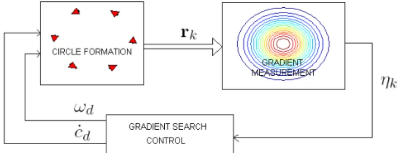
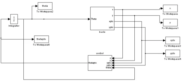
The following diagram of the general system points out the mainly objective, the gradient search. Even then we must build the formation control in order to achieve the control motion of the multi-agent system depending on the concentration measurements.
Figure 1: General system diagram
It is going to be attempted generalize the proposed problem. It would be useful to be able to construct control law with additive properties as the ones in the potential function approaches, where the various control capabilities are obtained by adding, or changing the potential functions. However, we have taken into account the time limitations for the development of all previous items and that this work Commande d’une flottille de robots sous-marines avec des constraints de communication, included in the CONNECT project, constitutes the background work for the thesis Control Design for Multi-Agent systems under communication constraints, we have followed a methodology more specific that highlights the main aspects of the project.
1. Formation Model 2. Control Formation
3. Transformations of the circle Formation (a) Translation
(b) Contraction (c) Rotation 4. Gradient Search
4
Formation Control
After the first mouth of the project, carrying out the review of the state of the art, we concluded that a kinematic model, as the model explained in [3], is appropriate for this system:
˙
rk = veiθk (7)
˙
θk = uk (8)
Henceforth, this model is used to represent the multi-agents system and all mathematical calculations take into account these equations. Although these equations can be simplified if we consider v= 1.
4.1 Circle Formation
According to the paper [3], the circle formation is possible through the application of only control law that depends on each agent. Thus, when the system becomes stable, all agents follows a circular trajectory the radius ρ= 1/ω0.
This control law is obtained applying the Lyapunov second theorem on stability to the following Lyapunov function candidate:
S(r, θ) = 1 2 N X k=1 |veiθk−iω 0˜rk|2
where ˜rk =rk−R defines the relative distance between the position of each agent rk and
the centre of mass of the formation R. If the aim is building a fixed circle, the equation ˙R= 0 is verified.
4.1.1 Circle with centre in (0,0)
In order to simplify the first implementation of the model, it is consider R= (0,0), hence the centre of circle formation will be in the origin of coordinate system.
Developing the Lyapunov theorem: ˙ S(r, θ) = N X k=1 [< veiθk −iω
0˜rk,−iω0r˙k>+< veiθk −iω0˜rk, iveiθkθ˙k>]
˙ S(r, θ) = N X k=1 <r˙k−iω0˜rk, ir˙k>(uk−ω0) Choosing the control law as follows
uk =ω0(1 +κh˜rk,r˙ki)
the system is stable because ˙ S(r, θ) =−κ N X k=1 hω0˜rk,r˙ki260
therefore Lyapunov stability theorem is proved.
The program Matlab and its application Simulink give us a suitable simulation environment. The simulations deal with understand the theoretical equations and permit an appropriate anal-ysis of the stability.
• Simulation Parameters
There are many parameters in the system equations and in the control law that have influence on simulation results. The time of convergence, system stability and the shape of the formation depend on the parameters values.
r0: The initial conditions determines the duration of transitory response until achieve a stable formation. Besides, the final relative heading value of each agent is generated according to the initial conditions. We have carried out several simulations with random initial conditions. All of them were stables.
n: The value of n represents the number of agents in the simulation. This is the main parameter to analyze the convergence time of the system. The convergence is faster with small values of n. An usual number of agents used in the simulations is four.
v: This is the speed of each agent. The circle radius is defined as ωv
0 thus v determines the formation size.
ω0: This is a parameter of the control law. Due to the previous equation, the radius of the circle depends on ω0. On the other hand, the system stability is conditioned too but this influence depends mainly on the relation with κ. We have chosen ω0 = 1 in almost all simulations.
κ: This parameter appears on the control law hence it has influence on the system stability. After several simulations it is concluded that the better values for this parameter is
κ=ω0 = 1 thus the convergence time is reduced. For higher values likeκ= 10 each agent carries out a circular motion with bigger radius therefore convergence time is increased. Whereas the values asκ= 0.1 produces independent circular motion with smaller radius for each agent. The convergence time is increased this time because the independent motion predominates over the part of the control law that search the final stable circle.
• Stability
Before, the stability of the system has been proved using the Lyapunov second theorem. Nevertheless it is worth mentioning that only control law is used and the speed of each agent is considered constant. Thus the agents must penetrate in the final stable trajectory through the several exterior circumferences.
In order to observe the system stability in the simulation, we have programmed a MATLAB file that generate an animation in real-time. The measurement of relative headings and relative angular velocity enhances the system stability.
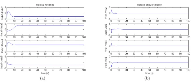
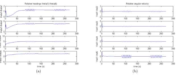
The following figures show the procedure of control law convergence, through the relative measurements of θk and ˙θk:
Each termθk−θj converges to a constant value because all agents have a fixed distribution
in the final stable circle. Moreover, for each agent the relative angular velocity ˙θk−θ˙j
converges to zero due to all agents track the same circular trajectory and turn with the same angular velocity. Thus all previous subtractions will be zero when the system becomes stable.
(a) (b)
Figure 2: (a) Relative headings (b) Relative angular velocity
4.1.2 Circle with random coordinates of the centre
Following with the work developed in [3], the centre of mass is defined as R= 1 N N X j=1 rj
hence the relative position of each agent can be expressed as follows: ˜ rk=rk−R= 1 N N X j=1 rkj where rkj =rk−rj.
The control law obtained is the same that in the case of the centre in (0,0). The main difference in the simulation results is the convergence time and obviously, the coordinates of the formation centre. The centre of the final stable circle depends on the initial conditions. The agents attempt to build a circle based in the centre of mass in each instant. Therefore the centre of stable circle will be positioned near the first system’s centre of mass that initial conditions establish. This is the reason for the faster stability in this second case.
4.1.3 Circle with centre in (c1, c2)
In order to make progress in the methodology proposed, we contribute in the project development applying a variation in the model definition. The centre of mass is defined as a complex number R =c1+ic2. This change permits controlling the position of the circle because c1 and c2 are the coordinates of the centre. Henceforth, the centre of mass is called centre of the circle and its nomenclature is C, thus the definition of relative position changes: ˜rk=rk−C
The simulation results are the same than in the case of circle with centre in (0,0). All simulation parameters have identical influence for the two cases.
The main different in this model is that we can choose the centre of the final circle. This is an advantage for the later approach than we want to move the formation.
4.2 Uniform Distribution
The control formation has been developed in several ways. The simulations show the applica-bility and staapplica-bility of each control law. After that, the following step is to achieve the uniforme distribution of all agents in the formation. According to the paper [3], a potential function can be added to the formation control law for control the relative-headings.
The stability analysis begins modifying the Lyapunov function candidate. An other objective function is defined as follows:
V(r, θ) =κS(r, θ) +U(θ) Differentiating ˙ V(r, θ) =κS˙(r, θ) +∂U ∂θθ˙ ˙ V(r, θ) = N X k=1 κ < ω0˜rk, ir˙k>(ω0−uk) + ∂U ∂θ ˙ θ ˙ V(r, θ) = N X k=1 [κ < ω0˜rk, ir˙k>(ω0−uk) + ∂U ∂θk ˙ θk]
The function U(θ) has an important quality:
<∇U,1>= 0 that is equivalent to N X k=1 ∂U ∂θk = 0
If this property is applied the previous equation can be expressed as: ˙ V(r, θ) = N X k=1 [κ < ω0˜rk, ir˙k>− ∂U ∂θk ˙ θk](ω0−uk)
Thus the control law changes as follows:
uk =ω0(1 +κh˜rk,r˙ki)−∂θ∂Uk where ∂θ∂U k is defined as: ∂U ∂θk =−K N N X j=1 [N/2] X m=1 sinmθkj m and θkj =θk−θj.
• Simulation Parameters
previous parameters: In this case, each previous parameter has the same influence in the convergence time, stability or radius value that in the formation control law.
K: This constant determines the weight of the relative heading control opposite the for-mation control. Theκ/K relation will decide what part has preference. Usually it is chosen a slow value for the relative heading control asκ= 10K because it is the equi-librated relation to improve the convergence. If K is ten times bigger, the uniform distribution is faster than circle formation. The system takes a longtime to form the final stable circle. In other hand, ifK is too small, the final circle will be formed quick but achieving the correct relative headings is more difficult due to the constant speed of all agents. The agents are forced to track several circular trajectories external to the final circle until the uniform distribution is completed.
• Stability
We are going to use a Matlab animation and the measurement of relative headings and relative angular velocity in order to analyze the system stability.
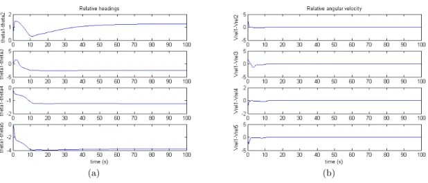
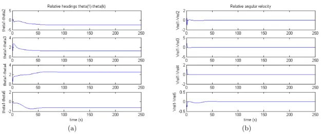
Again, for each agent the relative angular velocity ˙θk−θ˙j converges to zero due to all
agents track the same circular trajectory and turn with the same angular velocity. Each term θk−θj converges to a constant value because all agents have a fixed distribution
in the final stable circle. Nevertheless, the relative-heading control determines the value of each term. The value of relative heading must represent a uniform distribution in the circle, thus for each agent θk−θj = 2Nπ(k−j) where N is the number of agents in the
system.
The following figures show the procedure of control law convergence, through the relative measurements of θk and ˙θk:
(a) (b)
Figure 3: (a) Relative headings. (b) Relative angular velocity.
r0 n v ω0 κ K
random 2 to 12 1 0.5 to 2 1 0.1
5
Variable Formation Control
The control of variations in the circle formation is a previous step before the gradient search. The development of this new approach begins gathering all the information of the review of state of the art.
5.1 Main Transformations
The final objective is to steer the formation until it finds the source searched depending on the concentration measures. This task only can be achieved if the formation carries out the basic motions in the plane (due to it is considered two-dimensional problem). The formation motion is composed to three main transformations:
1. Translation
2. Contraction and Expansion 3. Rotation
Translation A translation is moving every point a constante distance in a specific direction. The translation motion can also be interpreted as the movement that change the position of an object.
A circle undergos a translation when the coordinates of its centre changes the value and the radius remain constante. Thus, the translation can be carried out controlling the value of (c1, c2)
Contraction and Expansion A contraction or expansion is changing the size of the formation without changing its shape. In a circle this transformation depends on its radius. When the radius is reduced, it is called contraction and the expansion is an increase of its radius. Then, this transformation can be controlled changing ω0 = 1/ρ.
Rotation A rotation is a movement which keeps a point fixed. This definition applies to an ellipse can be interpreted as the change of the orientation of every point keeping a focus fixed. Nevertheless, in a circle, any change keeping the centre fixed results the same circle. Then, we are not going to consider this transformation.
5.2 Limitation of the previous schemes
The first idea for check the ability of the system achieving transformations and variations, is to deal with change the simulation parameters directly. The constant parameters which have influence in the circle transformations areω0, it determines the radius of the circle, andCthan represents the coordinates of its centre. We must to simulate each transformation separately thus the influence of each variation in the system stability can be analyzed.
With the simulation results and the analysis of the control law and model equation, we can conclude that there is a transitory response when we impose an abrupt variation in the circle parameters ω0 and C. We show these conclusions here below.
5.2.1 Transitory response
The control law described previously for the circle formation can’t keep the system stability while a sudden variation is applied to the variables ω0 andC. This is, if the parameters change quickly, the formation is destroyed during the contraction or translation respectively.
Nevertheless the control law is able to achieve the objective. if the aim is the formation of a circle with bigger or smaller radius or if it is the formation of the circle with others coordinates of the centre, finally the system is stable.
With these results, we think that this system can reach the stability despite the perturba-tions. Our objective is to verify if the system is stable subject to soft variaperturba-tions.
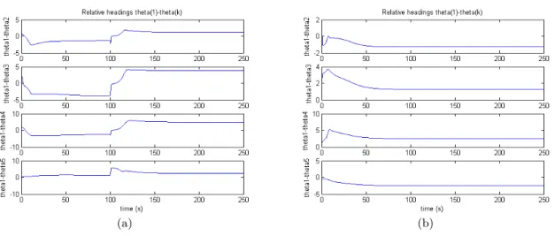
The measurement of the relative headings determines the stability of the system. We have made several simulations to show the transitory response. After attaining the stable formation, we introduce a variation step in the parameters for t= 100seconds. In the circle contraction, the variation is produced from ω0 = 0.3 toω0 = 1.5. The simulation for change the coordinates of the centre the variation is from (−1,−1) to (2,2). We can observe that the relative headings change suddenly. Although after the transitory response the system becomes stable.
Surprisingly, the expansion of the circle is more stable than the contraction.
The duration of the transitory response depends mainly on the number of agents. All these results are shown in the followings figures:
(a) (b)
Figure 4: (a) Relative headings for sudden variation in(c1, c2). (b) Relative heading for sudden variation inω0.
5.2.2 Slow variations
After the previous results, we are going to apply softer variations. Each variation is simulated individually and then, both transformations will be analyzed together.
Translation The coordinates of centre are new input variables for the system. The transfor-mation is carried out introducing a soft ramp instead of a value constant for c1 and c2.
Figure 5: Circle translation. The figure shows the formation during its translation motion between the two stable positions initial and final.
This ramp is attenuated by means of a second order filter which avoids the sudden changes that can affect the formation stability. The simulation results are satisfactory. The translation of the circle is produced without lost of the stability. That is, the formation is conserved during the motion.
(a) (b)
Figure 6: (a) Relative headings during translation motion. (b) Relative angular velocity during translation motion.
Depending on the slope of the ramp the system keeps the stable value for the relative headings. If the ramp is too hard the formation is conserved but the agents stop having an uniform distribution.
Contraction and Expansion In this other variation analysis, the aim is change the radius of the circle ρ= 1/ω0. Then,ω0 is a new input variable for the system. Again the transformation is carried out introducing a soft ramp asω0value. This ramp is attenuated by means of a second order filter which avoids the sudden changes that can affect the formation stability.
Figure 7: Contraction and Expansion of the circle. The figure shows the formation during the contraction motion between the two stable position initial and final.
The simulation shows that the circle is stable during the contraction and expansion motion. The formation and relative headings are conserved.
As the previous transformation (translation), depending on the slope of the ramp the system keeps the stable value for the relative headings. If the ramp is too hard the formation is conserved
but the agents stop having an uniform distribution.
(a) (b)
Figure 8: (a) Relative headings during contraction motion. (b) Relative angular velocity during contraction motion.
This figures shows that the circle keeps the relative headings during the contraction transfor-mation. The system is really stable although the perturbations in the value ofω0 are introduced. Combined Motions To conclude this section, we present the simulation results for the com-bined motions. Both transformations separately have resulted feasible and the system is stable for the two cases. If the translation and contraction are produced in the same simulation the system is still stable. The formation conserves the uniform distribution of the agents in the circle during all combined motion. Whit this conclusions we have come to the end of the slow variations section. From here on we can develop the gradient search using ω0 and (c1, c2) as system perturbations which permits the control of circle motion.
5.3 Control Redesign based on previous schemes
The stability and performances of the system have been analyzed introducing externals pertur-bations. The conclusion is that the control law is efficient for carry out the transformations of the circle but we want to control the transformation parameters directly. The following step is redesign a control law that permits including the variation of the parameters ω0 and (c1, c2) in the control closed-loop.
We search to achieve a contribution in the multi-agents and formation control fields. This is a mainly objective, as the formation control, analyzed previously, in this project.
At the beginning we are going to develop the control law for the contraction and expan-sion due to the previous results which shows that the system is more stable with this kind of transformation.
5.3.1 Contraction Algorithm
According to the section Formation Control, we search a Lyapunov function candidate which represents the stability objective. In this case, the parameter ω0 is variable then, henceforth, it is called ωd. We choose the previous Lyapunov function but now it depends onωd:
˙ V(r, θ, ωd) =κS˙(r, θ, ωd) + ∂U ∂θk ˙ θk where S(r, θ, ωd) = 1 2 N X k=1 |eiuk−iω d˜rk|2
Using the following notation: f(rk, θk, ωd) =eiuk−iω0˜rkthe derivative of previous function
is defined as: ˙ S(r, θ, ωd) = N X k=1 < f(rk, θk, ωd), ∂f(rk, θk, ωd) ∂rk ˙ rk >+ N X k=1 < f(rk, θk, ωd), ∂f(rk, θk, ωd) ∂θk ˙ θk>+ N X k=1 < f(rk, θk, ωd), ∂f(rk, θk, ωd) ∂ωd ˙ ωd>
Calculating all partial derivatives, the development of the Lyapunov theorem continues: ˙ S(r, θ, ωd) = N X k=1 <r˙k−iω0r˜k, iωgr˙k>+ N X k=1 < f( ˙rk−iω0˜rk, ir˙kθ˙k>+ N X k=1 < f( ˙rk−iω0˜rk,−i˜rkω˙d>
The two first terms can be merged as the formation control obtaining: ˙ S(r, θ, ωd) = N X k=1 < ωd˜rk,r˙k >(ωd−uk)+ ˙ ωd N X k=1 (<r˙k,−i˜rk>+<−iωd˜rk,−i˜rk >)
Therefore the derivative of Lyapunov function can be expressed as: ˙ V(r, θ, ωd) =κ N X k=1 < ωd˜rk,r˙k>(ωd−uk) + ∂U ∂θk ˙ θk+κω˙d N X k=1 (<r˙k,−i˜rk>+<−iωd˜rk,−i˜rk >)
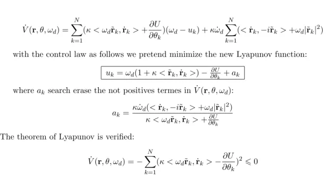
˙ V(r, θ, ωd) = N X k=1 (κ < ωd˜rk,r˙k>+ ∂U ∂θk )(ωd−uk) +κω˙d N X k=1 (<r˙k,−i˜rk>+ωd|˜rk|2)
with the control law as follows we pretend minimize the new Lyapunov function:
uk=ωd(1 +κ <˜rk,r˙k>)−∂θ∂Uk +ak
whereak search erase the not positives termes in ˙V(r, θ, ωd):
ak=
κω˙d(<r˙k,−ir˜k>+ωd|˜rk|2)
κ < ωd˜rk,r˙k >+∂θ∂Uk
The theorem of Lyapunov is verified: ˙ V(r, θ, ωd) =− N X k=1 (κ < ωd˜rk,r˙k>− ∂U ∂θk )260
We are going to make several simulations in the order to verify the control law obtained for the contraction of the circle. The simulink model (see attached document), consists of the formation control model and we add the new control term ak.
Again the transformation is carried out introducing a soft ramp as ω0 value. This ramp is attenuated by means of a second order filter which avoids the sudden changes that can affect the formation stability. It is necessary to include an other filter to obtain ˙ωd since it is an input
variable in the new term of the control law.
Figure 9: Contraction control. This figure shows the formation during the contraction motion between the two stable position initial and final. The circle don’t keep the uniform distribution.
The simulation results show that the system is finally stable because it is able to achieve the aim (change the radius of the formation) but during the motion, the circle loses the uniform distribution. The relative headings are kept only if the ramp is too soft.
Analyzing several times the equations which composes the Lyapunov method, we have not found calculation mistakes. Thus the simulations results are unsatisfactory due to two possible causes:
1. Implementation mistakes in the program code. The Matlab file and the simulink model have been debugged for one week. Even so, it has not been found obvious mistakes to conclude that it is the reason.
2. Concept error. It is possible that some hypothesis used in the calculation of the formation control is not true any more considering ωd variable.
6
Gradient Search Method
The gradient research is the main challenge of this project. We have develop the control laws previous for the circle formation and the analysis of the variation formation with the idea of moving the circle according to the measurement of each agent.
In order to develop the control for the gradient research we make a change of coordinates as follows:
Figure 10: Change of coordinates
Equation for each agent: ˙ rk = veiθk ˙ θk = ωd(1 +κ <r˜k,r˙k>)− ∂U ∂θk
Stable circle formation system: ˙ rk = veiψeiθ ∗ k (9) ˙ ψ = ωd (10) whereθ∗k= 2πkN−1
This new system can be considered because two reasons: When the circle formation is stable, all relative headings converges to zero, therefore ∂θ∂U
k converges to zero too. The second
reason is that the formation control law can be separated in two parts: ωd is the slow term and
We choose a change of coordinate system turning with the same angular speed ωd of each
agent and its origin is in the coordinates of the centre of the circle formation (c1, c2).
b
rk = ˜rke−iψ (11)
˙
b
rk = r˙˜ke−iψ−iψ˙˜rke−iψ (12)
And finally if we define ˙cde−iψ=bc˙d the new equation model is:
˙ brk =ve iθ∗ k−bc˙d−iωd b rk
The Lyapunov function, that we want to maximize this time, depends on the measurements of each agent, called ηk. The objective is to approach the values of measurements to the highest
source value. Hence, it is attempted to achieve the purpose using this function:
V(η) = 1 2 N X k=1 η2k Differentiating ˙ V(η) = N X k=1 ηkη˙k
Due to that, each measurement is a real number but the gradient of the concentration function is a vector, we have to introduce the definition as follows for the derivative of measurements:
˙ ηk(brk) =< ∂ηk ∂brk ,br˙k>=< ∂ηk ∂brk , veiθ∗k−bc˙d−iωd brk>
in such a way that it is possible to tackle the Lyapunov derivative: ˙ V(η) = N X k=1 ηk< ∂ηk ∂brk , veiθ∗k >+ N X k=1 ηk< ∂ηk ∂brk ,−bc˙d>+ωd N X k=1 ηk < ∂ηk ∂brk ,−brk> If we define ωd= N X k=1 ηk< ∂ηk ∂brk ,−brk>
a quadratic term is obtained in the Lyapunov function ˙V(ηk).
Moreover we can separate the others terms in their real components for search a control equation forbc˙d as follows:
N X k=1 ηk < ∂ηk ∂brk ,−bc˙d>=− N X k=1 ηk[ ∂ηk ∂brk |xbc˙dx+ ∂ηk ∂brk |ybc˙dy]
Thus it seems logical to define the two real components that they forms an other quadratic term:
bc˙dx = − N X k=1 ηk ∂ηk ∂brk |x (13) bc˙dy = − N X k=1 ηk ∂ηk ∂brk |y (14)
Although, the real components equations are going to be used for simulate, it is possible to find a complex expression: bc˙d=− N X k=1 ηk ∂ηk ∂brk
The complex equation permits achieving the change of coordinate system readily:
bc˙d= ˙cke−iψ ⇒c˙d=bc˙deiψ
However it is necessary to define the concentration gradient for obtaining it in the coordinates of original system: ∂ηk ∂brk = ∂ηk ∂rk ∂rk ∂brk = ∂ηk ∂rk eiψ
with this definition the expression for the control of the centre:
˙ cd=−eiψ N X k=1 ηk ∂ηk ∂rk eiψ = N X k=1 ηk ∂ηk ∂rk ei2ψ ˙ cdx = − N X k=1 ηk[ ∂ηk ∂rk |xcos 2ψ− ∂ηk ∂rk |ysin 2ψ] (15) ˙ cdy = − N X k=1 ηk[ ∂ηk ∂rk |ycos 2ψ+ ∂ηk ∂rk |xsin 2ψ] (16)
Nevertheless there is a not quadratic term in the Lyapunov function. The influence of this third term is unknown.
˙ V(η) = [− N X k=1 ηk ∂ηk ∂brk |x]2+ [− N X k=1 ηk ∂ηk ∂brk |y]2+ [ N X k=1 ηk< ∂ηk ∂brk ,−brk >]2+ N X k=1 ηk< ∂ηk ∂brk , veiθ∗k >
7
Conclusions
This project consist of two main objectives, the gradient search and the formation control that permits to carry out this search. We have explained previously the different steps to achieve each aim. Despite that the review of the state of the art developed supplies the necessary information to tackle each approach, we have reduced the items according to the durations of the project.
As it has been explained in the introduction, this project represents a thesis blackout. The thesis will tackle the approaches and challenges that this project has not been able to achieve.
7.1 Review of results
We summarize the simulation results and the mathematical conclusions presented in the previous sections, here below.
Formation control Choosing the system model and its representation mathematical, the development of formation control begins. We have followed the paper [3] obtaining a control law for a circle formation. The main challenge has been to understand every aspects of the Lyapunov stability theorem and its development. The understanding of these questions has permitted to attempt new control laws.
The control law used determines a stable formation for the four cases analyzed and simulated with satisfactory results:
1. Circle with centre in (0,0)
2. Circle with random coordinates of centre 3. Circle with centre in (c1, c2)
4. Uniform distribution, that is applicable to the three previous cases and the system con-tinues stable.
Variation control Introducing slow variations of the parametersω0and (c1, c2) the simulation results show that the stability of the system is conserved. Thus it is possible to use these parameters as input variables to control the gradient search.
We have developed a new contraction law. This control law is obtained applying the Lya-punov method, but the simulation results show lost of stability during the transformation. Gradient search The main difficulty is to achieve a suitable approach to develop the control law which carries out the gradient search. Working on the mathematical equations we have found a possible control law. This law is obtained with verify the Lyapunov stability theorem. The simulation results don’t show a stable system and the gradient search is only carried out with fixed parameters. This control law is not very robust.
7.2 Perspectives
Applying the satisfactory results obtained the following step is to complete the project by means of the thesis Control Design for Multi-Agent systems under communication constraints. This project supplies the mathematical base and the appropriated simulation environment for the development of several items:
• Improvement of the variation control laws (contraction and translation).
• To achieve a robust control law for the gradient search.
• Development of new models assuming communication constraints. According to the paper [5] the better solution is a graph model.
• To include a term in the formation control for the collision avoidance. The flocking algo-rithm seems more appropriate for the AUVs.
8
Review in French
8.1 Introduction
8.1.1 Contexte de stage
La communaut´e scientifique dans le domaine du contrˆole s’est focalis´ee principalement dans la commande de la formation des v´ehicules. Cependant, les syst`emes de coop´eration sont apparus comme sujets d’int´erˆet importants les derni`eres ann´ees.
Le stage est inclus dans le projet CONNECT, lequel a ´et´e fond´e par the ARN (National Research Agency. Le projet traite le probl`eme de la commande de syst`emes compos´es des plusieurs sous-syst`emes connect´es entre eux grˆace `a une reseau de communication h´et´erog`ene. Le principal objectif est d’apprendre comment on peut dessiner des lois de contrˆole en train de pr´eserver la stabilit´e du syst`eme en boucle ferm´e. Le project CONNECT appartient `a l’´equipe NeCS (Networked Controlled System Team) lequel est un ensemble des laboratoires INRIA et GIPSA-lab soutenus par CNRS, INRIA, INPG et UJF.
Dans le cas pr´ecis de ce stage, on cherche `a aborder le probl`eme du contrˆole des multi-agents syst`emes avec des contraintes de communication. On veut r´eussir `a ce qu’une flottille d’agents sous-marins travaillent en collaboration, pour r´ealiser la recherche (par gradient) et la localisation d’une source (eaux douce, source chimique, source de m´ethane, etc.). Chaque AUV est ´equip´e d’un capteur qui mesure la concentration de la source, et d’un syst`eme de communication (sonar) pour ´echanger des donn´ees relatives `a leur position absolue. L’objectif de la commande est de commander la flottille `a fin de r´ealiser la tˆache d’inspection d´ecrite pr´ec´edemment sous des contraintes de communication.
8.1.2 Etude de l’´etat de l’art
On commence avec la r´ealisation d’une ´etude de l’´etat de l’art. Nous allons r´esumer les travaux les plus caract´eristiques sur le domaine du contrˆole de syst`emes distribu´es, contrˆole d’une for-mation et d’algorithmes pour rechercher le gradient, ci-dessous.
Mod`eles On a trouv´e plusieurs mod`eles pour repr´esenter le mouvement des agents. Ils peu-vent ˆetre formul´es en trois dimensions, mais pour simplifier, on va utiliser les mod`eles en deux dimensions trait´es dans [1, 2, 3].
Mod`eles cin´ematiques: Beaucoup d’´etudes r´ealis´ees dans le domaine du contrˆole des syst`emes multi-agent proposent des mod`eles simples . On trouve principalement des mod`eles avec une masse ponctuelle du type: ˙xi =ui ou mod`eles lin´eaires. Cependant, pour les
appli-cations concernant les robots sous-marins, il semble qu’un mod`ele non lin´eaire est plus appropri´e [3]:
˙
rk = veiθk (17)
˙
Mod`eles dynamiques: Ces mod`eles sont moins utilis´es dˆus `a leur complicit´e. Ils tiennent compte de la force appliqu´ee `a l’agent, [1].
Mod`eles pour un groupe: On introduit nouvelles variables pour d´ecrire le mouvement du groupe. Le centre de masse est d´efini en [3]: R= N1 PN
j=1rk
Contrˆole de la formation On montre quelques strat´egies pour la commande de la formation. On consid`ere que tous les agents peuvent communiquer avec tous les autres.
1. Contrˆole bas´e sur Lyapunov
Mouvement circulaire et distribution uniforme: L’article [3] propose la loi du contrˆole suivant pour accomplir les deux objectives:
˙ uk =ω0(1 +κh˜rk,r˙ki) | {z } cicular−control − ∂U ∂uk |{z} relative−headings (19)
Cette loi est obtenue en appliquant le th´eor`eme de stabilit´e de Lyapunov. Groupes coordonn´ees.
Commande pour une forme d´etermin´ee. 2. Algorithmes bas´es sur Laplacien
Gossip: C’est un protocole qui est dessin´e pour imiter la perte d’information quand les agents font des comm´erages pour les mettre en relation avec les contraintes de com-munication.
Consensus: On d´efinit les concepts graphe et voisins pour un ensemble d’agents. Le graphe permet de connaˆıtre les relations de communication de chaque agent avec ses voisins.
Contrˆole d’une formation distribu´ee.
3. Contrˆole qui ´evite les obstacles Flocking, mot d´efini en [12], c’est une forme qui repr´esente un groupe d’agents connect´es entre eux avec un objectif commun. Cet algorithme utilise le contrˆole de consensus pour d´efinir les obstacles de fa¸con `a ce qu’ils soient consid´er´es comme de nouveaux voisins dans le graphe.
Contrˆole pour chercher une source Il y a plusieurs travaux qui traitent de la recherche d’une source. On trouve principalement les mod`eles de la source qui suivent une ´equation diffusive.
Formations avec une forme d´eformable: On essaie d’ajuster cette forme aux courbes de niveau de la source.
Adaptation `a la croissance du gradient: On d´etermine une fonction objective pour la recherche du gradient qui sera maximis´ee.
8.2 M´ethodologie
Apr`es avoir r´euni les diff´erents approches sur le contrˆole des syst`emes multi-agents on confec-tionne la m´ethodologie n´ecessaire pour d´evelopper ce stage. Les objectifs propos´es sont d´etaill´es ensuite:
1. Mod`ele de la formation 2. Contrˆole de la formation 3. Transformations du cercle
(a) Translation (b) Contraction
(c) Rotation
4. Recherche du gradient
8.3 Contrˆole de la formation
On se fonde sur les ´etudes r´ealis´ees en [3] pour accomplir le premi`ere objectif propos´e dans la m´ethodologie pr´ec´edente.
Pour d´evelopper chaque section, on va effectuer une analyse th´eorique et une application pratique. On fera les simulations pour v´erifier les r´esultats obtenus, avec le program Matlab et Simulink.
8.3.1 Formation du cercle
Le mod`ele non lin´eaire suivant est consid´er´e pour repr´esenter notre syst`eme: ˙
rk = veiθk (20)
˙
θk = uk (21)
Apr`es ce choix on simule le syst`eme en boucle ferm´ee avec la loi de commande exprim´ee en [3] pour la formation du cercle:
uk =ω0(1 +κh˜rk,r˙ki)
ou ˜rk=rk−R.
Cette formule a ´et´e d´evelopp´ee grˆace au th´eor`eme de stabilit´e de Lyapunov, appliqu´e `a la fonction S(r, θ) = 1 2 N X k=1 |veiθk−iω 0˜rk|2
Les r´esultats des simulations montrent que la loi de commande utilis´ee est capable de former le cercle de radius ρ= 1/ω0 et stabiliser le syst`eme pour les trois cas suivants:
Cercle avec centre en (0,0): Pour obtenir le cercle en l’origine de coordonn´ees, il faut annuler le centre de masse du syst`eme R=0. Les valeurs des angles relatifs sont constantes par cons´equent la formation est stable.
Cercle avec coordonn´ees al´eatoires du centre: On d´efinit le centre de masseR= N1 PN
j=1rk.
Le centre du cercle d´epend des conditions initiales. Dˆu `a cette definition, le syst`eme r´eussit `
a ˆetre stable plus rapidement.
Cercle avec centre en (c1, c2): Les r´esultats des simulations sont ´egaux que dans le premier cas. Portant, affiner la definition du centre de masse comme cela R = C permettra d’accomplir la translation du cercle.
8.3.2 Distribution uniforme
Une fois qu’on a r´eussi `a contrˆoler la formation, le but suivant est distribuer les agents de fa¸con uniforme dans le cercle. On peut r´ealiser cette tˆache rien qu’en ajouter un terme `a la loi de commande:
uk=ω0(1 +κhr˜k,r˙ki)−
∂U ∂θk
o`u ce terme est d´efini comme suit:
∂U ∂θk =−K N N X j=1 [N/2] X m=1 sinmθkj m et θkj =θk−θj.
On d´eduit cette expression parce qu’on a introduit une nouvelle fonction potentielle dans la fonction de Lyapunov:
V(r, θ) =κS(r, θ) +U(θ)
Les simulations r´ealis´ees pour ce cas montrent que le syst`eme est stable et encore les angles relatifs v´erifient θk−θj = 2Nπ(k−j) o`u N est le nombre d’agents. Par cons´equent, les agents
ont une distribution uniforme dans le cercle.
8.4 Contrˆole des variations de la formation
Les principaux transformations qu’on peut r´ealiser dans une formation sont: 1. Translation
2. Contraction 3. Rotation
Pourtant, pour un cercle la rotation n’a aucun sens, donc on va considerer seulement les deux premi`eres transformations.
R´eponse transitoire: On commence en analysant les r´eponses du syst`eme par rapport les variations des param`etresω0 et les coordonn´ees du centre. On conclut que si les variations de ces param`etres sont brusques, le syst`eme arrˆete d’ˆetre stable pendant le transformation. Variations lentes: Par cons´equent, l’objectif suivant est d’´evaluer la stabilit´e en introduisant des variations doucement. Apr`es avoir r´ealis´e plusieurs simulations on peut affirmer que chaque transformation est accomplie sans perdre la stabilit´e avec une ´etendue marge de variation des param`etres. De plus la distribution uniforme est conserv´ee autant pour la translation que pour la contraction.
Contrˆole de la contraction: Bien qu’on a r´eussi `a d´eplacer la formation et `a changer sa forme, on veut inclure le contrˆole des transformations dans la boucle ferm´ee du syst`eme global. On a contribu´e en d´eveloppant une loi de commande qui essaie de faire stable le syst`eme pendant la contraction si on consid`ereω0=ωdvariable. La fonction de Lyapunov
pour analyser la stabilit´e est ´egale `a l’ant´erieure mais quand on derive, il faut deriver sur
ωd. Finalement on obtiens:
uk=ωd(1 +κ <r˜k,r˙k >)−
∂U ∂θk
+ak
o`u ak cherche `a ´eliminer les terms n´egatifs dans la d´eriv´ee de la fonction de Lyapunov
˙ V(r, θ, ωd): ak = κω˙d(<r˙k,−ir˜k>+ωd|˜rk|2) κ < ωd˜rk,r˙k>+∂θ∂U k
Cependant les simulations montrent que le syst`eme devient instable pendant la transfor-mation.
8.5 Recherche du gradient
Une fois qu’on a r´ealis´e la commande de la formation d’une mani`ere satisfaisante, l’objectif essentiel est de chercher une m´ethode pour accomplir la recherche du gradient.
Les param`etres ωd et (c1, c2) peuvent ˆetre consid´er´es variables d’entr´ee au syst`eme. On va d´evelopper une loi de commande pour chaque param`etre en d´ependant des measures de la concentration pris pour les agents. Pour ce faire, on propose une changement des coordonn´ees du syst`eme qui tourne avec une vitesse angulaire ´egale `a la rotation de chaque agent dans le cercle: b rk = ˜rke−iψ (22) ˙ b rk = r˙˜ke−iψ−iψ˙˜rke−iψ (23)
On d´efinit une nouvelle mod`ele pour le cercle stable: ˙ rk = veiψeiθ ∗ k (24) ˙ ψ = ωd (25)
o`uθ∗k= 2πkN−1.
Avec ces ´equations on cherche `a maximiser la fonction de Lyapunov:
V(η) = 1 2 N X k=1 η2k
puisque vers la source, les valeurs des mesures ηk seront plus grandes. Donc, si la fonction de
Lyapunov grandit, ¸ca veut dire qu’on s’approche `a la source.
Apr`es plusieurs calculs on trouve les suivants lois de commande pour chaque param`etre:
ωd = N X k=1 ηk< ∂ηk ∂brk ,−brk > (26) ˙ cd = − N X k=1 ηk ∂ηk ∂rk eiψ (27)
il faut tenir compte de changement des coordonn´ees:
∂ηk ∂brk = ∂ηk ∂rk ∂rk ∂brk = ∂ηk ∂rk eiψ
Mais ces formules ne r´eussissent pas rendre positifs tous les termes de la fonction de Lya-punov, c’est-`a-dire, on ne peut pas assurer la stabilit´e du syst`eme.
Effectivement, les simulations ne sont pas satisfaisantes. On a trouv´e une combinaison de param`etres qui accomplit la recherche du gradient. C’est la raison pour laquelle on consid`ere que la loi de commande obtenu est pr`es d’ˆetre la solution mais il faut analyser attentivement les calculs et am´eliorer l’impl´ementation des simulations.
8.6 Conclusions
Ce projet permet d’analyser plusieurs facettes diff´erentes dans le domaine du syst`emes multi-agents. On a appris `a d´evelopper la m´ethode de Lyapunov pour chercher la lois de commande qui fait stable le system. Les formules th´eoriques ont ´et´e appliqu´ees d’une mani`ere satisfaisante pour le contrˆole de la formation du cercle. Les lois de commande utilis´ees gardent la formation stable et la distribution uniforme mˆeme si les param`etres, ω0 et les coordonn´ees du centre, varient doucement.
On a trouv´e difficult´es pour accomplir la recherche du gradient dˆu `a la complexit´e des ´equations qui repr´esentent le syst`eme comme un cercle stable et aussi dˆu au probl`eme de d´efinir la valeur du gradient grˆace `a les mesures pris pour chaque agent.
Ce stage constitue l’ensemble des connaissances pour d´evelopper la th`ese dans le mˆeme domaine qui nous occupera les trois prochaines ann´eesControl Design for Multi-Agent systems under communication constraints. Par cons´equent, toutes les simulations non satisfaisantes seront analys´ees au mˆeme temps qu’on aborde les diverses approches pour le probl`eme des contraintes de communication.
9
Attached Document A
9.1 Operators
Operator <, > inner product:
a,b∈CN therefore the operator is defined as:
<a,b>=Re{aTb}
This definition can be used for developer the derivate of the same kind functions witch we use as Lyapunov functions.
If V = |f(ϕ)| 2 2 = 1 2(f(ϕ)f(ϕ)) where f :RN →CN then ˙ V = ∂ ∂t[ 1 2(f(ϕ)f(ϕ))] = 1 2[ ˙f(ϕ)f(ϕ) +f(ϕ) ˙ f(ϕ)] 9.2 Calculations developed 9.2.1 Formation Control
In order to obtain the formation control law, we apply the Lyapunov second theorem on stability to the following Lyapunov function candidate:
S(r, θ) = 1 2 N X k=1 |veiθk−iω 0˜rk|2
where ˜rk =rk−R defines the relative distance between the position of each agent rk and the
centre of mass of the formation R.
Using the following notation f(rk, θk) =veiθk −iω0˜rk then
S(r, θ) = 1 2 N X k=1 |f(rk, θk)|2
and the derivative of the previous function is defined as: ˙ S(r, θ) = N X k=1 < f(rk, θk), ∂f(rk, θk) ∂rk ˙ rk>+ N X k=1 < f(rk, θk), ∂f(rk, θk) ∂θk ˙ θk> Partial derivatives: ∂f(rk, θk) ∂rk = −iω0 ∂f(rk, θk) ∂θk = iveiθk =ir˙ k
and we have defined previously ˙θk=uk, therefore ˙ S(r, θ) = N X k=1 < f(rk, θk),−iω0r˙k>+ N X k=1 < f(rk, θk), ir˙kuk> < f(rk, θk),−iω0r˙k> = −ω0 < f(rk, θk),−iω0r˙k > < f(rk, θk), ir˙kuk> = < f(rk, θk), ir˙k> uk then ˙ S(r, θ) = N X k=1 < f(rk, θk), ir˙k >(uk−ω0) = N X k=1 < veiθk −iω 0˜rk, ir˙k>(uk−ω0) = N X k=1 <r˙k−iω0˜rk, ir˙k>(uk−ω0) = N X k=1 [<r˙k, ir˙k>−ω0 < i˜rk, ir˙k>](uk−ω0) = Operating: <r˙k, ir˙k>=Re{r˙k T ir˙k}= Re{( ˙xk−iy˙k)i( ˙xk+iy˙k)}= Re{ix˙2k−x˙ky˙k) + ˙xky˙k) +iy˙k)2}= 0 < i˜rk, ir˙k>=Re{i˜rk T ir˙k}= Re{(−x˜k−y˜k)i( ˙xk+iy˙k)}= Re{x˜kx˙k+ix˜ky˙k)−iy˜kx˙k) + ˜yky˙k)}=<˜rk,r˙k> Finally ˙ S(r, θ) = N X k=1 [<r˙k, ir˙k >−ω0< i˜rk, ir˙k >](uk−ω0) = N X k=1 [0−ω0 <˜rk,r˙k>](uk−ω0) = N X k=1 [ω0 <˜rk,r˙k>](ω0−uk)
9.2.2 Uniform Distribution Control
In order to obtain the uniform distribution formation control law, we combine the previous circular control law with a potential control term:
uk=ω0(1 +κhr˜k,r˙ki)−
∂U ∂θk
The new Lyapunov function candidate is composed by two terms:
V(r, θ) =κS(r, θ) +U(θ) Differentiating ˙ V(r, θ) =κS˙(r, θ) +∂U ∂θ ˙ θ= N X k=1 κ < ω0˜rk, ir˙k>(ω0−uk) + ∂U ∂θk ˙ θ= N X k=1 (κ < ω0˜rk, ir˙k>(ω0−uk) + ∂U ∂θk uk)
Due to the property
<∇U,1>= 0 N X k=1 ∂U ∂θk = 0 ω0 N X k=1 ∂U ∂θk = 0 we obtained ˙ V(r, θ) = N X k=1 [κ < ω0˜rk, ir˙k>(ω0−uk) + ∂U ∂θk uk]−ω0 N X k=1 ∂U ∂θk = N X k=1 [κ < ω0˜rk, ir˙k>(ω0−uk) + ∂U ∂θk (uk−ω0)] = N X k=1 [κ < ω0˜rk, ir˙k>− ∂U ∂θk ](ω0−uk)
If we defined the uniform distribution control law as
uk=ω0(1 +κhr˜k,r˙ki)− ∂U ∂θk Operating ˙ V(r, θ) = N X k=1 [κ < ω0˜rk, ir˙k >− ∂U ∂θk ](ω0−(ω0(1 +κh˜rk,r˙ki)− ∂U ∂θk )) =
N X k=1 [κ < ω0˜rk, ir˙k>− ∂U ∂θk ](ω0−ω0−κ < ω0˜rk,r˙k >+ ∂U ∂θk ) = N X k=1 [κ < ω0˜rk, ir˙k>− ∂U ∂θk ](−κ < ω0˜rk,r˙k>+ ∂U ∂θk ) = − N X k=1 [κ < ω0˜rk, ir˙k>− ∂U ∂θk ]2 Finally ˙ V(r, θ) =− N X k=1 [κ < ω0˜rk, ir˙k>− ∂U ∂θk ]2 60
9.3 Contraction circle control
We need to control ω0, therefore we define ω0 = ωd. Then §depends on ωd now. The new
Lyapunov function is:
V(r, θ, ωd) =κS(r, θ, ωd) +U(θ)
and its derivative is expressed as follows: ˙ V(r, θ, ωd) =κS˙(r, θ, ωd) + ∂U ∂θk ˙ θk
Differentiating the first term: ˙ S(r, θ, ωd) = N X k=1 < f(rk, θk, ωd), ∂f(rk, θk, ωd) ∂rk ˙ rk >+ N X k=1 < f(rk, θk, ωd), ∂f(rk, θk, ωd) ∂θk ˙ θk>+ N X k=1 < f(rk, θk, ωd), ∂f(rk, θk, ωd) ∂ωd ˙ ωd> Partial derivatives: ∂f(rk, θk, ωd) ∂rk = −iωd ∂f(rk, θk, ωd) ∂θk = iveiθk =ir˙ k ∂f(rk, θk, ωd) ∂ωd = −i˜rk Operating ˙ S(r, θ, ωd) = N X k=1 <r˙k−iω0r˜k, iωgr˙k>+
N X k=1 < f( ˙rk−iω0˜rk, ir˙kθ˙k>+ N X k=1 < f( ˙rk−iω0˜rk,−i˜rkω˙d>= N X k=1 < ωd˜rk,r˙k>(ωd−uk)+ ˙ ωd N X k=1 (<r˙k,−i˜rk>+<−iωd˜rk,−i˜rk>) = N X k=1 < ωd˜rk,r˙k>(ωd−uk)+ ˙ ωd N X k=1 (<r˙k,−i˜rk>+ωd|˜rk|2)
Therefore the derivative of Lyapunov function can be expressed as: ˙ V(r, θ, ωd) = N X k=1 [κ < ωd˜rk,r˙k >(ωd−uk) + ∂U ∂θk uk] +κω˙d N X k=1 (<r˙k,−i˜rk>+ωd|˜rk|2) = N X k=1 [κ < ω0˜rk, ir˙k>− ∂U ∂θk ](ω0−uk) +κω˙d N X k=1 (<r˙k,−i˜rk>+ωd|˜rk|2)
with a control law as follows
uk=ωd(1 +κ <r˜k,r˙k>)− ∂U ∂θk +ak we simplifies ˙ V(r, θ, ωd) = N X k=1 [κ < ωd˜rk, ir˙k>− ∂U ∂θk ](ωd−(ωd(1 +κ <˜rk,r˙k>)− ∂U ∂θk +ak))+ κω˙d N X k=1 (<r˙k,−i˜rk>+ωd|˜rk|2) = N X k=1 [κ < ωd˜rk, ir˙k >− ∂U ∂θk ](ωd−ωd−κ < ωd˜rk,r˙k>+ ∂U ∂θk −ak)+κω˙d N X k=1 (<r˙k,−i˜rk >+ωd|˜rk|2) = N X k=1 [κ < ωd˜rk, ir˙k >− ∂U ∂θk ](−κ < ωd˜rk,r˙k>+ ∂U ∂θk −ak) +κω˙d N X k=1 (<r˙k,−i˜rk>+ωd|˜rk|2) = − N X k=1 [κ < ωd˜rk, ir˙k >− ∂U ∂θk ]2+ N X k=1 (κ < ωd˜rk, ir˙k>− ∂U ∂θk )(−ak)+
κω˙d N
X
k=1
(<r˙k,−i˜rk>+ωd|˜rk|2)
We search erase the two last terms:
N X k=1 (κ < ωd˜rk, ir˙k>− ∂U ∂θk )(−ak) +κω˙d N X k=1 (<r˙k,−i˜rk>+ωd|˜rk|2) = 0 Hence ak= κω˙d(<r˙k,−ir˜k>+ωd|˜rk|2) κ < ωd˜rk,r˙k >+∂θ∂Uk
and the Lyapunov second theorem on stability is verified: ˙ V(r, θ) =− N X k=1 [κ < ω0˜rk, ir˙k>− ∂U ∂θk ]2 60
9.4 Gradient Search Control law
Equation for each agent: ˙ rk = veiθk ˙ θk = ωd(1 +κ <r˜k,r˙k>)− ∂U ∂θk
when the circle formation is stable uk →u∗k then formation system can be defined by:
˙
r∗k = veiψeiθ∗k (28)
˙
ψ = ωd (29)
where θk∗ = 2πkN−1
We define the new relative position variablebrk for each agent
brk= (rk+cd)e
−iψ =r
ke−iψ+cde−iψ
and for simplicity we consider bcd=cde−iψ, then
b rk=rke−iψ+bcd its derivative is ˙ b rk= ˙rke−iψ−iψ˙rke−iψ+ ˙bcd=ve
iθke−iψ−iω
drke−iψ+ ˙bcd=ve
−iθ∗k−iω
d(ˆrk−cd) + ˙bcd
and the measurements of the agent kis expressed in function of the position of each vehicle