Composite Differential Evolution for Constrained Evolutionary Optimization

(1)

Composite Differential Evolution for Constrained

Evolutionary Optimization

Bing-Chuan Wang, Han-Xiong Li

, Fellow, IEEE

, Jia-Peng Li, and Yong Wang

, Senior Member, IEEE

Abstract—When solving constrained optimization problems by

evolutionary algorithms, the search algorithm plays a crucial role. In general, we expect that the search algorithm has the capability to balance not only diversity and convergence but also constraints and objective function during the evolution. For this purpose, this paper proposes a composite differential evolution for constrained optimization, which includes three different trial vector generation strategies with distinct advantages. In order to strike a balance between diversity and convergence, one of these three trial vector generation strategies is able to increase diversity, and the other two exhibit the property of convergence. In addition, to accomplish the tradeoff between constraints and objective function, one of the two trial vector generation strategies for convergence is guided by the individual with the least degree of constraint violation in the population, and the other is guided by the individual with the best objective function value in the population. After producing offspring by the proposed composite differential evolution, the feasibility rule and the ε constrained method are combined elaborately for selection in this paper. Moreover, a restart scheme is proposed to help the population jump out of a local optimum in the infeasible region for some extremely complicated constrained optimization problems. By assembling the above techniques together, a constrained composite differential evolution is proposed. The experiments on two sets of benchmark test functions with various features, i.e., 24 test functions from IEEE CEC2006 and 18 test functions with 10 dimensions and 30 dimensions from IEEE CEC2010, have demonstrated that the proposed method shows better or at least competitive performance against other state-of-the-art methods.

Index Terms—constrained optimization, evolutionary

algorith-m, composite differential evolution, constraint-handling tech-nique

I. INTRODUCTION

This work was supported in part by a General Research Fund (GRF) project from Research Grant Council (RGC) of Hong Kong SAR (CityU: 11205615), in part by the Project from the City University of Hong Kong under Grant 7004666, in part by the Innovation-Driven Plan in Central South University under Grant 2018CX010, in part by the National Natural Science Foundation of China under Grant 61673397, and in part by the Hunan Provincial Natural Science Fund for Distinguished Young Scholars (Grant No. 2016JJ1018). (Corresponding author: Yong Wang).

B.-C. Wang is with the Department of Systems Engineering and Engineering Management, City University of Hong Kong, Hong Kong. (e-mail: [email protected]).

H.-X. Li is with the Department of Systems Engineering and Engineering Management, City University of Hong Kong, Hong Kong, and also with the State Key Laboratory of High Performance Complex Manufacturing, Central South University, Changsha 410083, China. (e-mail: [email protected]).

J.-P. Li is with the School of Information Science and Engineering, Central South University, Changsha 410083, China. (e-mail: [email protected]).

Y. Wang is with the School of Information Science and Engineering, Central South University, Changsha 410083, China, and also with the School of Computer Science and Electronic Engineering, University of Essex, Colchester CO4 3SQ, UK. (Email: [email protected]).

C

ONSTRAINTS are everywhere. Many practical opti-mization problems, such as vehicle configuration de-sign [1], scheduling [2], [3], digital circuit structure dede-sign [4], mixed-model two-sided assembly line [5], and antenna de-sign [6], can be formulated as constrained optimization prob-lems (COPs). Hence, how to solve COPs is of great practical significance.

As a kind of population-based heuristic optimization al-gorithms, evolutionary algorithms (EAs) [7] have attracted increasing interest in solving COPs. As a result, a variety of constrained EAs has been proposed [8], [9], [10]. A constrained EA includes two main components: 1) search algorithm and 2) constraint-handling technique. Search algo-rithm plays the role of generating new candidate solutions, and thus has a significant impact on the performance of constrained EAs. During the past two decades, differential evolution (DE) [11] has become one of the most popular EA paradigms. DE has numerous attractive advantages. First of all, its structure is simple and it can be implemented easily in any programming language. In addition, it includes few control parameters. Moreover, it has already achieved top ranks in a lot of competitions at IEEE Congress on Evolutionary Computation (IEEE CEC). Note that no other single algorithm can accomplish this [12]. More importantly, its search ability has been demonstrated in many real-world applications [13], [14], [15].

Due to the above advantages, DE has been frequently applied to solve COPs. Two primary ways of utilizing DE for constrained optimization can be summarized as: 1) designing a new DE, or 2) extending an existing DE originally designed for global optimization to deal with constrained optimization. In terms of case 2), many DE variants for global optimization have been tailored to tackle COPs [16], [17], [18], [19]. As an outstanding global optimizer, composite differential evolution (CoDE) [20] exhibits a few strengths, including ease of implementation, powerful search ability, integrating the strengths of different trial vector generation strategies, etc. However, few current studies investigate CoDE for constrained optimization.

Motivated by the above consideration, this paper seeks to make use of the idea of CoDE to solve COPs. The underlying idea behind CoDE is the utilization of three different trial vector generation strategies of DE with a variety of character-istics to address the key issue of global optimization, i.e., the tradeoff between diversity and convergence. In order to extend CoDE to tackle COPs, the tradeoff between constraints and objective function should also be taken into account. To this end, this paper proposes a constrained composite differential

(2)

evolution, called C2oDE, to address these two issues. Similar to CoDE, C2_{oDE also contains three different trial} vector generation strategies with distinct advantages. Specifi-cally, one trial vector generation strategy for diversity and two trial vector generation strategies for convergence are employed to balance diversity and convergence. In addition, one of the two trial vector generation strategies for convergence is guided by the individual with the least degree of constraint violation while the other is guided by the individual with the best objective function value, with the aim of balancing constraints and objective function. During the evolution, these three trial vector generation strategies are used to generate three offspring for each target vector. Afterward, a new comparison rule, which combines the feasibility rule with the ε constrained method, is proposed. Herein, the feasibility rule is applied to preselect the best one from the three offspring as the trial vector. Due to the fact that the feasibility rule prefers constraints, the εconstrained method, which can incorporate the information of objective function to a certain degree, is used to compare each target vector with its trial vector. Therefore, the new comparison rule can further promote the balance between constraints and objective function. Moreover, a restart scheme is designed to help the population jump out of a local optimum in the infeasible region for some extremely complex COPs.

By combining the strengthes of the above-mentioned tech-niques, C2oDE achieves a reasonable tradeoff between diver-sity and convergence as well as between constraints and objec-tive function. The contributions of this paper are summarized as follows:

• The principle of CoDE is successfully applied to design a search algorithm for constrained optimization.

• The feasibility rule and theεconstrained method are inte-grated in an effective way to select promising individuals for the next population.

• A restart scheme is proposed to cope with COPs with extremely complicated constraints.

• Systematic experiments have demonstrated that C2_oDE provides state-of-the-art performance on two benchmark test suites.

The rest of this paper is organized as follows. Section II introduces the preliminary knowledge. The related work on constrained DE is reviewed in Section III. Section IV illus-trates the proposed method in detail. Extensive experiments and discussions are carried out in Section V. Section VI concludes this paper.

II. PRELIMINARYKNOWLEDGE

A. Constrained Optimization Problems (COPs)

Without loss of generality, a COP [21], [22] can be de-scribed as follows:

minimize f(~x), ~x= (x1, ..., xD)∈S, Li≤xi ≤Ui subject to : gj(~x)≤0, j= 1, ..., l

hj(~x) = 0, j=l+ 1, ..., m

wheref(~x)is the objective function,~xis the decision vector, xiis theith dimension of~x,LiandUiare the upper and lower bounds of xi, respectively, D is the number of dimensions,

S = QD

i=1[Li, Ui] represents the decision space, gj(~x) is the jth inequality constraint, l is the number of inequality constraints, hj(~x) is the (j −l)th equality constraint, and

(m−l)is the number of equality constraints.

For COPs, the degree of constraint violation of the decision vector~xcan be expressed as follows:

G(~x) =

m

X

j=1

Gj(~x) (1)

whereGj(~x)is the degree of constraint violation on the jth constraint and calculated as follows:

Gj(~x) =

max(0, gj(~x)), 1≤j≤l

max(0,|hj(~x)| −δ), l+ 1≤j≤m (2) In Equation (2),δis a positive tolerance value to relax equality constraints to a certain extent.~xis called a feasible solution if G(~x) = 0. The aim of solving COPs is to locate the optimum in the feasible region.

B. Differential Evolution (DE)

The unique feature of DE is to make use of differential vectors to generate offspring [12], [23]. In general, DE consists of four stages, i.e., initialization, mutation, crossover, and selection.

Firstly, an initial population including N P target vectors (also calledN P individuals) is randomly generated from the decision space. In the mutation stage, a mutation operator is implemented to generate a mutant vector for each target vector~xt

i(i∈ {1, . . . , N P})at generationt. Several mutation operators have been proposed. As a representative, DE/rand/1 is described as follows:

~

vt_i =~xt_r₁+F·(~xt_r₂−~xt_r₃) (3) where ~vt

i is the mutant vector of the ith target vector ~xti, ~ xt r1, ~x t r2, and ~x t

r3 are three mutually distinct target vectors

randomly selected from the population, and F is the scaling factor. Some other popular mutation operators are enumerated as follows: • DE/rand/2 ~vit=~x t r1+F·(~x t r2−~x t r3) +F·(~x t r4−~x t r5) (4) • DE/rand-to-best/1 ~v_it=~xt_r 1+F·(~x t best−~x t r1) +F·(~x t r2−~x t r3) (5) • DE/current-to-best/1 ~vt_i =~xt_i+F·(~xt_best−~xt_i) +F·(~xt_r 1−~x t r2) (6) • DE/current-to-rand/1 ~vt_i =~x_it+rand·(~xt_r 1−~x t i) +F·(~x t r2−~x t r3) (7) where ~xtr1, ~x t r2, ~x t r3, ~x t r4, and~x t

r5 are five mutually distinct

target vectors randomly selected from the population,~xt_best is the best target vector in the current population, andrandis a uniformly distributed random number between 0 and 1.

Different mutation operators have distinct characteristics. DE/rand/1 is the most commonly used mutation operator in the

(3)

t i x 1 t i u 2 t i u t i u t i x 1 t i x preselection trial vector generation strategy II 3 t i u selection

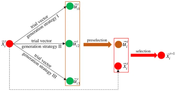
Fig. 1. Framework of CoDE.

DE community [20], in which all individuals are selected in a random manner for mutation. Due to the fact that an additional differential vector is utilized, DE/rand/2/ can provide a better perturbation than DE/rand/1. By making use of the information of the best individual, both DE/rand-to-best/1 and best/1 can speed up the convergence. In DE/current-to-rand/1, each target vector learns from a randomly selected individual, thus promoting the diversity.

In the crossover stage, a crossover operator is conducted on each pair of ~xt

i and~vti to produce a trial vector ~uti. The frequently used binomial crossover is introduced below:

uti,j =

vt

i,j, ifrandj < CRorj =jrand xt

i,j, otherwise

(8) where ut

i,j, xti,j, and vi,jt are the jth dimension of ~uti, ~xti, and ~vt

i, respectively, randj is a random number uniformly generated between 0 and 1, CR is the crossover control parameter, andjrandis a random integer uniformly generated between 1 and D.

Finally, a selection operator is performed on~xt

i and~uti, and the better one is selected as the target vector of the (t+ 1)th generation. ~ xt_i+1= ~ ut_i, iff(~u_it)≤f(~xt_i) ~ xt_i, otherwise (9)

In DE, a combination of a mutation operator and a crossover operator is called a trial vector generation strategy.

Currently, DE has been successfully applied to solve opti-mization problems in a considerable number of fields, such as electrical and power systems [24], [25], manufacturing science and operational research [26], [27], automotive design [28], and controller design [13], [14], [15].

C. CoDE

CoDE is one of the top DE variants proposed by Wang et al. [20] for global optimization. The main idea of CoDE is to combine several effective trial vector generation strategies with several appropriate DE parameter settings, which show complementary characteristics, to improve DE’s performance. In CoDE, a strategy pool comprised of three well-studied trial vector generation strategies, i.e., DE/rand/1/bin, DE/rand/2/bin, and DE/current-to-rand/1, is constructed in advance. On the other hand, a parameter pool involving three pairs of F andCR is constructed beforehand: [F=0.8;

CR=0.2], [F=1.0;CR=0.1], and [F=1.0;CR=0.9]. As depicted in Fig. 1, three offspring, i.e.,~ut

i1,~u

t i2, and~u

t

i3, are generated

for each target vector ~xt

i via implementing the three trial vector generation strategies in the strategy pool one by one. Moreover, each trial vector generation strategy is associated with a pair ofF andCRrandomly chosen from the parameter pool. Subsequently, the best one among the three offspring is preselected as the trial vector ~ut_i. Finally, the better one between~xt_i and ~ut_i is selected as the potential individual for the next generation.

By utilizing distinct advantages of different trial vector gen-eration strategies and parameter settings, CoDE accomplishes outstanding performance. Owing to its simple structure, ease of implementation, and effectiveness, CoDE is fully investi-gated for constrained optimization in this paper.

D. Feasibility Rule

The feasibility rule proposed by Deb [29] is a well-known constraint-handling technique. It compares pairwise individuals as follows:

1) Between two infeasible individuals, the one with less degree of constraint violation is preferred.

2) If one individual is feasible and the other is infeasible, the feasible one is preferred.

3) Between two feasible individuals, the one with a smaller objective function value is preferred.

E. εConstrained Method

The ε constrained method proposed by Takahama and Sakai [30], [31] is another representative constraint-handling technique. When comparing two individuals, say ~xt

i and ~xtj, ~

xt

iis better than~xtj if and only if the following conditions are satisfied:    f(~xi)< f(~xj), ifG(~xi)≤ε∧G(~xj)≤ε f(~xi)< f(~xj), ifG(~xi) =G(~xj) G(~xi)< G(~xj), otherwise (10)

In Equation (10),εdeclines as the generation increases: ε= ε0(1−_Tt)cp, if _Tt ≤p 0, otherwise (11) cp=−logε0+λ log(1−p) (12)

whereε0 is the initial threshold and set to be the maximum degree of constraint violation of the initial population,T is the maximum generation number,λis set to 6 in this paper, andp

controls the degree that the information of objective function is exploited.

III. RELATEDWORK

DE has become a very popular search engine for constrained optimization and this paper focuses mainly on constrained DE (CDE). In this section, we survey the development of CDE primarily during the last five years and classify CDE into three classes: 1) single-strategy CDE, 2) multi-strategy CDE, and 3) CDE coupled with other operators. For a more comprehensive review, the interested reader can refer to [32].

(4)

A. Single-Strategy CDE

As suggested by the name, single-strategy CDE signifies that CDE just includes one trial vector generation strategy.

For example, De Melo and Carosio [33] conducted an empirical analysis on five classical trial vector generation strategies which are separatively integrated with a simple penalty function. According to the experimental results, they claimed that classical DE with a simple penalty function is still very competitive.

In [19], the famous global optimizer JADE [34] is combined with an archiving-based adaptive tradeoff model [35] for constrained optimization.

Gaoet al.[36] suggested a dual population scheme in which one population is responsible for tackling constraints and the other for optimizing objective function. Moreover, a modified DE/rand/1/bin is designed to share the information between two populations.

Takahama and Sakaia [37] presented an efficient CDE. Through utilizing kernel regression, this method has the capability to find approximately optimal solutions with a very small number of function evaluations. In addition, the ε constrained method serves as the constraint-handling technique and DE/rand/1 with exponential crossover operator serves as the search algorithm. Yiet al.[38] presented anεconstrained DE with pre-estimated comparison based on gradient-based approximation for solving COPs.

Wang and Cai [39] proposed a dynamic hybrid framework referred as DyHF for constrained optimization. In DyHF, the global and local search models are dynamically imple-mented according to the feasibility proportion of the current population. In the same year, Wang and Cai [40] combined multiobjective optimization with DE and proposed CMODE. In CMODE, an infeasible solution replacement mechanism based on multiobjective optimization is devised to guide the population toward promising solutions and the feasible region simultaneously. Note that both DyHF and CMODE exploit Pareto dominance [41] to compare individuals.

Hamza et al. [42] integrated a DE with multi-constraint consensus. In this method, the constraint consensus [43] aims at moving the infeasible solutions along the parallel direction to the violated constraint, thus making them feasible quickly. The constraint consensus has also been used in [44].

In the self-adaptive interior penalty based DE [45], the scaling factor F and crossover control parameter CR of DE/rand/1/bin are adjusted according to the success rate. Fan and Yan [46] also developed a self-adaptive penalty based DE. However, the two DE control parameters, i.e., F and CR, together with the penalty factor, are adapted in the manner of coevolution by the alopex algorithm [47]. In [48], a fuzzy rule based penalty function approach is designed. Li and Zhang [49] showed that a modified penalty method, called minimum penalty method, is effective to handle constraints.

It is necessary to emphasize that for [38], [39], [40], [42], [45], [46], [48], and [49], DE/rand/1/bin is directly employed as the search algorithm.

B. Multi-Strategy CDE

In contrast to the first class, a number of CDE involves multiple trial vector generation strategies as pinpointed by the name.

For instance, Dong et al. [17] combined CoDE [20] with oracle penalty function to solve COPs. Herein, CoDE is treated as the search algorithm in a straightforward way.

Long et al. [50] integrated three trial vector generation strategies, i.e., DE/rand/1/bin, DE/best/1/bin, and DE/current-to-rand/1 to evolve the population. In this method, the initial population is divided into three sub-populations with equal size, and then each sub-population is assigned with a trial vector generation strategy to update the individuals.

De Melo and Carosio [51] provided a systematic way to ensemble five trial vector generation strategies, in which each trial vector generation strategy is applied to generate a corresponding solution and winner-take-all paradigm is utilized to select the best one as the trial vector.

By taking advantage of the concept of multi-population evolution, a cultural DE is developed in [52], in which each population is managed by its private cultural DE.

In [53], DE/rand/1/bin is employed in the early stage for exploration while DE/rand/1 with exponential crossover operator is adopted in the later stage for exploitation.

Jia et al. [35] divided the evolutionary process into three situations, i.e., the infeasible situation, the semi-feasible situa-tion, and the feasible situation. In different situations, different constraint-handling techniques are developed: multiobjective optimization for the infeasible situation and adaptive penalty function for the semi-feasible situation.

In [8], Wanget al.made use of DE/rand-to-best/1/bin to in-troduce information of objective function into the population. Meanwhile, DE/current-to-rand/1 is used to cope with rotated optimization problems.

Ghasemishabankareh et al. [54] exploited a popular DE variant (i.e., SaDE [55]) in a coevolution fashion and an improved augmented Lagrangian to deal with constraints.

Adaptive mechanisms are also used in multi-strategy CDE [56], where each trial vector generation strategy is adaptively selected according to its performance.

C. CDE Coupled with Other Operators

Recently, CDE coupled with other operators has also at-tracted much attention.

Dong and Wang [57] proposed a memetic DE for con-strained optimization, in which DE/rand/1/bin serves as the global search operator while the simplex crossover [58] plays the role of local search. To handle constraints, a weight sum method which somehow likes penalty method is designed.

In [59], the mixed-integer hybridizing DE is combined with the Nelder-Mead simplex method [60] to solve mixed-integer constrained optimization. Additionally, the Lagrange method and self-adaptive penalty function are incorporated to deal with constraints.

Zhao et al. [61] integrated three algorithms, in which DE is responsible for accelerating the convergence at the later iteration process of the backtracking search algorithm [62],

(5)

Diversity Tradeoff Convergence

Constraints Tradeoff Objective Function

DE/current-to-rand/1 modified DE/rand-to-best/1/bin DE/current-to-best/1/bin

Fig. 2. Principle of the designed search algorithm.

the mutation operator of the breeder genetic algorithm [63] is employed to improve the population diversity, and the parameter-free penalty method is used to handle constraints.

Parouha and Das [64] hybridized DE with particle swarm optimization for constrained optimization. In this method, the optimized population is divided into three parts. Afterward, DE is used to evolve two of them and particle swarm optimization is used for the remaining one.

In [65], DE is combined with an improved teaching-learning-based optimization algorithm to solve constrained engineering design problems.

Tranet al.[66] hybridized DE with artificial bee colony for solving resource-constrained project scheduling problems.

Our work in this paper falls in the second class, i.e., attempting to design a search algorithm with multiple trial vector generation strategies to solve COPs.

IV. PROPOSEDMETHOD

A. Motivation

When applying EAs to solve COPs, two issues deserve much attention in order to obtain outstanding performance: 1) the tradeoff between diversity and convergence, and 2) the tradeoff between constraints and objective function. At present, more and more DE variants originally proposed for global optimization have been extended to search for the optimal solutions of COPs, due to their excellent search ability. Note, however, that in global optimization the essential purpose of the search algorithm is to balance diversity and convergence. As a consequence, the performance of most current CDE is limited due to the fact that the tradeoff between constraints and objective function has been neglected unreasonably in the search algorithm.

In view of the above drawback, this paper aims to make use of the idea of CoDE [20], a state-of-the-art DE variant, to design a search algorithm for constrained optimization. As pointed out previously, the search algorithm and constraint-handling technique are two important aspects of a constrained EA. Therefore, we also present a constraint-handling technique to suit the characteristics of CoDE. Additionally, a restart scheme is designed to tackle COPs with extremely complicat-ed constraints. By assembling the above techniques together, an alternative CDE, i.e., C2oDE, is proposed in this paper.

Next, the search algorithm, constraint-handling technique, restart scheme, and framework of C2oDE are introduced one by one.

Algorithm 1: Search Algorithm

1 /*DE/current-to-rand/1*/ 2 Select~xt_r 1,~x t r2, and~x t

r3from the population;

3 Randomly choose aFvalue fromFpool; 4 ~vt i1=~xti+rand·(~xtr1−~x t i) +F·(~xtr2−~x t r3); 5 ~ut_i₁=~vt_i₁; 6 /*Modified DE/rand-to-best/1/bin*/ 7 Select~xt

Gbest(i.e., the individual with the least degree of constraint violation), ~ xt_r 1,~x t r2,~x t r3, and~x t

r4 from the population;

8 Randomly choose aFvalue fromFpooland aCRvalue fromCRpool; 9 ~vt i2=~xtr1+F·(~x t Gbest−~xtr2) +F·(~x t r3−~x t r4); 10 Generate~ut

i2by applying the binomial crossover on~v

t i2and~x t i; 11 /*DE/current-to-best/1/bin*/ 12 Select~xt

f best(i.e., the individual with the best objective function value),~xtr1,

and~xt

r2 from the population ;

13 Randomly choose aFvalue fromFpooland aCRvalue fromCRpool; 14 ~vt_i₃=~xt_i+F·(x~t_{f best}−~xt_i) +F·(~xt_r

1−~x

t r2);

15 Generate~ut

i3by applying the binomial crossover on~vti3and~xti;

B. Search Algorithm

An ideal search algorithm for constrained optimization should not only reach a balance between diversity and con-vergence, but also between constraints and objective function. For this purpose, similar to CoDE, the designed search algorithm depicted in Fig. 2 involves three different trial vector generation strategies with distinct advantages. They are DE/current-to-rand/1, modified DE/rand-to-best/1/bin, and DE/current-to-best/1/bin.

As mentioned before, with respect to DE/current-to-rand/1 shown in Equation (7), each target vector~xt

i learns the infor-mation from a randomly selected individual ~xt_r₁; therefore, this trial vector generation strategy is able to promote the diversity of the population. In principle, DE/current-to-rand/1 can be decomposed into two steps: 1) implementing DE/rand/1 to generate the mutant vector~vt_i for ~xt_i, and 2) applying the arithmetic crossover on~xt

i and~vitas follows:

~ut_i =~xt_i+rand·(~v_it−~xt_i) (13) where rand is a uniformly distributed random number on the interval [0,1]. As introduced in [20], [55], and [67], both DE/rand/1 and the arithmetic crossover are independent on the coordinate system and thus are rotation-invariant processes. As a result, DE/current-to-rand/1 is also beneficial to solve rotated optimization problems.

In terms of both the modified DE/rand-to-best/1/bin and DE/current-to-best/1/bin, the information of the “best” indi-vidual in the population is utilized to guide the search, thus accelerating the convergence. As shown in Equation (14), the modified DE/rand-to-best/1/bin is derived by replacing the second~xt

r1in Equation (5) with a randomly selected individual

~ xt

r2 from the population:

~

v_it=~xt_r₁+F·(~xt_best−~xt_r₂) +F·(~x_rt₃−~xt_r₄) (14) The reason for this modification is explained as follows. There are two trial vector generation strategies for conver-gence and one trial vector generation strategy for diversity in the search algorithm, which might result in more biases toward convergence than diversity. By this modification, the modified DE/rand-to-best/1/bin has the potential to produce more disturbances than the original one. Thus, the tradeoff

(6)

between diversity and convergence can be achieved in the search algorithm.

In addition, the “best” individual in the modified DE/rand-to-best/1/bin is chosen as the individual with the least de-gree of constraint violation while the “best” individual in DE/current-to-best/1/bin is selected as the individual with the best objective function value, with the aim of balancing constraints and objective function. Needless to say, the above balance is very important. It is because if the search is biased only toward constraints, the population might enter the feasible region with a very fast speed but subsequently converge to a local optimum in the feasible region due to the lack of diversity. On the other hand, the search biased only toward objective function would be very likely to get stuck in the infeasible region and could not find any feasible solution in the end. It should be noted that if multiple solutions have the same least degree of constraint violation or the same best objective function value, a random one is selected from them. Overall, the proposed search algorithm provides an effective way to achieve the two desired tradeoffs in constrained optimization, the details of which are given in Algorithm 1. As shown in Algorithm 1, three offspring will be generated for each target vector. Moreover, similar to [8], we establish two parameter pools Fpool andCRpool for the scaling factor F and the crossover control parameterCR, respectively.

C. Constraint-Handling Technique

In constrained evolutionary optimization, the constraint-handling technique is in charge of how to compare individuals. According to the characteristics of CoDE, the constraint-handling technique should include two phases as shown in Fig. 1: 1) how to preselect the best one from the three offspring as the trial vector, and 2) how to compare the target vector with its trial vector. According to the no free lunch theorem [68], [69] and [70], it is better to employ two different constraint-handling techniques rather than just one in the above two phases.

The feasibility rule is selected as one candidate owing to its attractive advantages, i.e., no additional parameters and the ability to rapidly motivate the population toward the feasible region. However, it is necessary to note that the feasibility rule prefers constraints to objective function and is a relatively greedy constrain-handling technique. Thus, we introduce the ε constrained method as the other candidate. From Equation (10), it can be seen that the ε constrained method also considers the information of objective function when comparing two individuals.

Obviously, there are two options to arrange these two constraint-handling techniques: 1) the ε constrained method in the first phase and the feasibility rule in the second phase, or 2) the feasibility rule in the first phase and theεconstrained method in the second phase. As shown in Fig. 1, the constraint-handling technique in the second phase determines which solution will survive into the next generation. In the case of option 1), the feasibility rule in the second phase might discard an individual with promising objective function value selected by theεconstrained method in the first phase. That is,

t i x 1 t i u 2 t i u t i u t i x 1 t i x modified DE/ rand-to-best/1/bin 3 t i u feasibility rule constrained method 

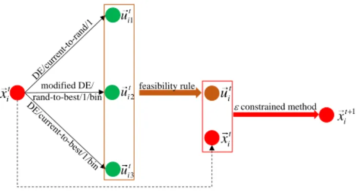
Fig. 3. Framework of C2oDE.

option 1) would make the population bias toward constraints ultimately. In the case of option 2), although some biases are introduced by the feasibility rule in the first phase due to its preference to constraints, the εconstrained method in the second phase attempts to balance such biases by exploiting the information of objective function. Moreover, the degree that the information of objective function is exploited can be controlled by the parameter pin Equation (12). In summary, option 2) is adopted in this paper.

D. Restart Scheme

For some COPs with extremely complicated constraints, the infeasible region is highly nonlinear and always exhibits multimodal property. Under this condition, the population is very easy to stagnate in the infeasible region. To address this issue, a restart scheme is proposed in this paper.

Prior to applying the restart scheme, we need to judge whether the population has already been trapped into a local optimum in the infeasible region. It is intuitive that if the population clusters in a very small search range of the infeasible region, which means the difference/similarity among infeasible individuals is very tiny/high, then we can claim that premature convergence occurs in the infeasible region. However, how to measure the similarity among infeasible individuals should be studied in depth.

A possible way is to compute the average Euclidean distance among all the individuals or the average standard deviation of all the dimensions of the population. If such indicator is less than a specified threshold, then one can conclude that the similarity among all the individuals is very high. Nevertheless, it is not trivial to set an appropriate threshold since different problems possess different dimensions and search spaces. Considering this, we use a unitary indicator, i.e., the degree of constraint violation or objective function value, to measure the similarity of the population. It is believed that this unitary indicator is less sensitive to different problems.

Consequently, if the standard deviation of the degree of constraint violation or the standard deviation of objective function values of the population is less than a predefined threshold µ and if the population is infeasible, the restart scheme is triggered – all the individuals in the population are regenerated from the decision space randomly without any special skills.

(7)

Algorithm 2: C2_oDE Input:N P: the population size

M axF Es: the maximum number of function evaluations Fpool: the pool of the scaling factorF

CRpool: the pool of the crossover control parameterCR 1 t=1; /*tdenotes the generation number*/

2 Randomly generate an initial populationPt={~xt1, ..., xtN P}from the decision spaceS;

3 Evaluate the objective function values and the degree of constraint violation of Pt;

4 F Es=N P; /*F Esdenotes the number of fitness evaluations*/ 5 Tune theεvalue of theεconstrained method according to Equation (11); 6 Pt+1=∅;

7 fori= 1 :N P do

8 Implement the search algorithm (Algorithm 1) to generate three offspring ~ ut i1,~u t i2, and~u t

i3for the target vector~x

t i;

9 Evaluate the objective function values and the degree of constraint violation of~ut

i1,~uti2, and~uti3;

10 Apply the feasibility rule to select the best one among~ut

i1,~uti2, and~uti3as

the trial vector~ut_ifor~xt_i;

11 Apply theεconstrained method to compare~xt

iand~uti, and store the better one intoPt+1;

12 F Es=F Es+ 3; 13 Implement the restart scheme; 14 t=t+ 1;

15 Stopping Criterion: IfF Es≥M axF Es, then stop and output the best individual inPt, otherwise go to Step 5.

E. C2oDE

By integrating three important components, i.e., the search algorithm, constraint-handling technique, and restart scheme, C2oDE is obtained. The framework of C2oDE is given in Fig. 3. C2oDE maintains a population consisting ofN P target vectors: Pt={~xt1, ~xt2, ..., ~xtN P}, their objective function val-ues: f(~xt

1), f(~xt2), ..., f(~xtN P), and their degree of constraint violation: G(~xt

1), G(~xt2), ..., G(~xtN P). As shown in Fig. 3, at generation t, three trial vector generation strategies are employed to generate three offspring (~ut

i1,~uti2, and ~uti3) for each target vector~xt

i. Afterward, the feasibility rule is used to preselect the best offspring as the trial vector ~ut

i. And then, the ε constrained method is utilized to compare ~xt_i and ~ut_i. Finally, the restart scheme is executed. The above procedure is repeated until the maximum number of fitness evaluations (M axF ES) is reached. The details of C2oDE are presented inAlgorithm 2. From Fig. 3 andAlgorithm 2, it can be seen that the implementation of C2oDE is simple.

Remark 1: Compared with other existing multi-strategy CDE, the advantages of C2oDE are summarized from the following three aspects:

• The search algorithm of C2oDE takes both the tradeoff between constraints and objective function and the trade-off between diversity and convergence into account. • Two well-known constraint-handling techniques with

complementary properties are combined in an effective way for selection.

• Its computational time complexity is the same with the classical DE without any additional computation burden.

V. EXPERIMENTALSTUDY

A. Benchmark Test Functions and Parameter Settings

Two sets of benchmark test functions were selected to assess the performance of C2oDE. The first set contains 24 test functions at IEEE CEC2006 [21], and the second set

TABLE I

MAXIMUMNUMBER OFFUNCTIONEVALUATIONSM axF EsAND

POPULATIONSIZEN P

Test Functions M axF Es N P

24 test functions from IEEE CEC2006 2.4E+05 50 18 test functions with 10D from IEEE CEC2010 2.0E+05 35 18 test functions with 30D from IEEE CEC2010 6.0E+05 60

contains 18 test functions with 10 dimensions (10D) and 30 dimensions (30D) at IEEE CEC2010 [22]. These 60 test functions can systematically investigate the performance of a constrained EA since they exhibit a variety of characteristics such as different dimensions of decision space, different types of objective function (i.e., linear, nonlinear, quadratic, polynomial, and cubic), and different kinds of constraints (i.e., linear/nonlinear and equality/inequality). All these test functions are minimization problems and their details can be found in [21] and [22].

For the experiments in this paper, the settings ofM axF Es and the population size N P are given in Table I. Note that a proper setting ofN P is related to the benchmark test suite as well as the dimension of a test function. In addition, 25 independent runs were performed for each test function and the tolerance valueδfor equality constraints was set to10−4_. As the same with [8], Fpool = [0.6, 0.8, 1.0] and CRpool = [0.1, 0.2, 1.0]. Meanwhile,pin theεconstrained method and µin the restart scheme were set to 0.5 and10−8_{, respectively.}

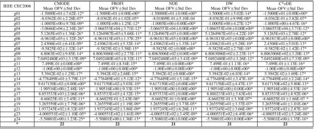
B. Experiments on IEEE CEC2006 Test Suite

Firstly, C2oDE was applied to solve 24 test functions from IEEE CEC2006. The performance of C2oDE was compared with that of four state-of-the-art CDE (i.e., CMODE [40], FROFI [8], NDE [71], and DW [72]). From [21], we know that it is extremely difficult to find a feasible solution for g22 and there are no feasible solutions for g20. Thus, we excluded these two functions and focused on the remaining 22 test functions. The experimental results are given in Table II, where “Mean OFV” and “Std Dev” denote the average and standard deviation of the objective function values obtained over 25 independent runs, respectively. For each test function, a run is successful if the following success condition is satisfied: f(~xbest)-f(~x∗)≤0.0001, where~x∗is the best-known solution and~xbest is the best feasible solution provided by a method. In Table II, “*” means that a method can satisfy the success condition in all 25 runs for a test function.

As shown in Table II, among the five compared CDE, CMODE, FROFI, and C2_{oDE successfully solve all the 22} test functions. NDE fails to consistently find the optimal solution of g02. DW cannot attain the optimal solution of g17 consistently. The experimental results demonstrate that, overall, C2_{oDE presents better or similar performance} compared with the four competitors on the 22 test functions from IEEE CEC2006.

C. Experiments on IEEE CEC2010 Test Suite

In this subsection, the performance of C2oDE was further tested by making use of other 36 test functions from IEEE

(8)

TABLE II

EXPERIMENTALRESULTS OFC2_O_DE_AND_O_THER_F_OUR_S_ELECTED_M_{ETHODS OVER}_{25 I}_NDEPENDENT_R_{UNS ON}_{22 T}_EST_F_{UNCTIONS FROM}_IEEE

CEC2006

IEEE CEC2006 _{Mean OFV}CMODE_±_{Std Dev} _{Mean OFV}FROFI_±_{Std Dev} _{Mean OFV}NDE_±_{Std Dev} _{Mean OFV}DW_±_{Std Dev} C 2_oDE Mean OFV±Std Dev g01 -1.5000E+01±7.62E-12* -1.5000E+01±0.00E+00* -1.50000E+01±0.00E+00* -1.5000E+01±5.02E-14* -1.5000E+01±0.00E+00* g02 -8.0362E-01±2.28E-07* -8.0362E-01±1.02E-05* -8.01809E-01±5.10E-04 -8.0362E-01±9.99E-08* -8.0362E-01±3.82E-07* g03 -1.0005E+00±9.78E-09* -1.0005E+00±1.25E-12* -1.0005E+00±0.00E+00* -1.0005E+00±4.27E-12* -1.0005E+00±4.67E-16* g04 -3.0666E+04±2.34E-26* -3.066553E+04±3.71E-12* -3.066553E+04±0.00E+00* -3.066553E+04±0.00E+00* -3.066553E+04±3.71E-12* g05 5.1265E+03±1.36E-26* 5.1264967E+03±5.68E-11* 5.1264967E+03±0.00E+00* 5.1264967E+03±4.22E-10* 5.1265E+03±2.78E-12* g06 -6.9618E+03±1.32E-26* -6.961813E+03±1.37E-25* -6.961813E+03±0.00E+00* -6.961813E+03±0.00E+00* -6.961813E+03±0.00E+00* g07 2.4306E+01±6.41E-09* 2.430621E+01±5.32E-14* 2.430621E+01±1.35E-14* 2.430621E+01±5.28E-10* 2.4306E+01±5.01E-13* g08 -9.5825E-02±1.32E-14* -9.5825E-02±3.58E-15* -9.5825E-02±0.00E+00* -9.5825E+02±2.78E-18* -9.5825E-02±1.42E-17* g09 6.8063E+02±9.85E-14* 6.8063006E+02±2.73E-11* 6.8063006E+02±0.00E+00* 6.8063006E+02±2.23E-11* 6.8063006E+02±3.20E-13* g10 7.0492480E+03±3.15E-09* 7.0492480E+03±8.32E-11* 7.0492480E+03±3.41E-09* 7.0492480E+03±3.26E-12* 7.0492480E+03±7.33E-09* g11 7.499E-01±0.00E+00* 7.499E-01±8.54E-15* 7.499E-01±0.00E+00* 7.499E-01±1.13E-16* 7.499E-01±1.13E-16* g12 -1.00E+00±0.00E+00* -1.00E+00±0.00E+00* -1.00E+00±0.00E+00* -1.00E+00±0.00E+00* -1.00E+00±0.00E+00* g13 5.3942E-02±1.25E-17* 5.3942E-02±2.68E-15* 5.3942E-02±0.00E+00* 5.3942E-02±6.03E-14* 5.3942E-02±1.69E-17* g14 -4.776489E+01±3.79E-11* -4.776489E+01±5.12E-12* -4.776489E+01±5.14E-15* -4.776489E+01±3.47E-10* -4.776489E+01±2.24E-14* g15 9.617150E+02±0.00E+00* 9.617150E+02±5.03E-10* 9.617150E+02±0.00E+00* 9.617150E+02±4.47E-13* 9.617150E+02±5.80E-13* g16 -1.90516E+00±2.48E-16* -1.90516E+00±9.33E-15* -1.90510E+00±0.00E+00* -1.90516E+00±0.00E+00* -1.90516E+00±4.53E-16* g17 8.853533E+03±2.06E-06* 8.853533E+03±4.32E-15* 8.853533E+03±0.00E+00* 8.880233E+03±3.63E+01 8.853533E+03±8.92E-06* g18 -8.66025E-01±3.45E-11* -8.66025E-01±2.43E-08* -8.66025E-01±0.00E+00* -8.66025E-01±3.30E-07* -8.66025E-01±1.66E-07 * g19 3.265559E+01±7.79E-06* 3.265559E+01±1.19E-09* 3.265559E+01±3.73E-05* 3.265559E+01±3.37E-07* 3.265559E+01±1.01E-06* g21 1.937245E+02±8.32E-05* 1.937245E+02±3.86E-09* 1.937245E+02±6.26E-11* 1.937245E+02±3.66E-09* 1.937245E+02±2.87E-10* g23 -4.000551E+02±1.10E-05* -4.000551E+02±1.61E-09* -4.000551E+02±3.45E-09* -4.000551E+02±6.49E-06* -4.000551E+02±5.24E-08* g24 -5.50801E+00±1.23E-25* -5.50801E+00±1.36E-13* -5.50801E+00±0.00E+00* -5.50801E+00±0.00E+00* -5.50801E+00±1.35E-16*

* 22 22 21 21 22

TABLE III

EXPERIMENTALRESULTS OFC2_O_DE_AND_O_THER_F_IVE_S_ELECTED_M_{ETHODS OVER}_{25 I}_NDEPENDENT_R_{UNS ON}_{18 T}_EST_F_{UNCTIONS WITH}_10D_FROM

IEEE CEC2010

IEEE CEC2010 with 10D CMODE

Mean OFV±Std Dev

FROFI

Mean OFV±Std Dev

ECHT-DE

Mean OFV±Std Dev

AIS-IRP

Mean OFV±Std Dev

Co-CLPSO

Mean OFV±Std Dev

C2oDE

Mean OFV±Std Dev

C01 -7.47E-01±2.35E-13+ -7.47E-01±1.35E-03+ -7.47E-01±1.40E-03+ -7.47E-01±1.30E-03+ -7.34E-01±1.78E-02− -7.44E-01±7.39E-03

C02 -1.48E+00±4.88E-01∇− -2.02E+00±1.41E-01− -2.27E+00±6.70E-03≈ -2.27E+00±2.00E-03≈ -2.27E+00±1.46E-02≈ -2.26E+00±4.64E-02

C03 2.84E+00±4.23E+00− 0.00E+00±0.00E+00≈ 0.00E+00±0.00E+00≈ 3.75E-09±4.81E-04− 3.55E-01±1.78E+00− 0.00E+00±0.00E+00

C04 -9.99E-04±2.90E-08− -1.00E-05±0.00E+00≈ -1.00E-05±0.00E+00≈ -9.97E-06±4.28E-03− 9.34E-06±1.07E-06− -1.00E-05±0.00E+00

C05 -4.50E+02±1.61E+02∇− -4.84E+02±8.09E-07≈ -4.11E+02±7.63E+01− -4.80E+02±6.30E+00− -4.84E+02±1.98E-02≈ -4.84E+02±3.48E-13

C06 -5.78E+02±1.60E-02− -5.79E+02±5.04E-04≈ -5.62E+02±4.51E+01− -5.80E+02±7.30E-08+ -5.79E+02±5.73E-04≈ -5.79E+02±6.17E-02

C07 6.69E-15±8.95E-15− 0.00E+00±0.00E+00≈ 1.33E-01±7.28E-01− 1.17E-08±2.70E+00− 7.97E-01±1.63E+00− 0.00E+00±0.00E+00

C08 8.94E+00±3.98E+00− 7.11E+00±4.79E+00≈ 6.16E+00±6.45E+00+ 4.09E+00±1.46E+00+ 6.09E-01±1.43E+00+ 7.30E+00±5.18E+00

C09 2.13E+06±1.04E+07∇− 2.50E+01±3.92E+01− 1.47E-01±8.05E-01+ 2.70E+01±7.50E+01− 1.99E+10±9.97E+10− 5.17E+00±5.19E+01

C10 1.35E+05±1.61E+06∇− 4.17E+01±8.69E-06− 1.71E+00±7.66E+00+ 1.62E+03±5.00E+02− 4.97E+10±2.49E+11− 3.67E+01±1.38E+01

C11 -7.7E-02±2.85E-02∇− -1.52E-03±5.63E-14≈ -4.40E-03±1.57E-02∇− -9.20E-04±8.23E-04− -1.61E-01±6.60E-01∇− -1.52E-03±4.89E-13

C12 -6.14E+02±2.74E+02∇− -3.84E+02±2.17E+02+ -1.72E+02±2.21E+02∇− -4.36E+02±6.02E+01+ -2.34E+00±2.43E+01− -7.63E+01±1.22E+02

C13 -5.79E+01±4.09E+00− -6.84E+01±2.52E-09≈ -6.51E+01±2.38E+00− -6.79E+01±3.11E-01− -6.53E+01±2.58E+00− -6.84E+01±2.77E-14

C14 8.18E-09±1.64E-08− 0.00E+00±0.00E+00≈ 7.02E+05±3.19E+06− 1.22E-04±2.90E-08− 3.19E-01±1.10E+00− 0.00E+00±0.00E+00

C15 1.20E+02±3.48E+02− 3.09E+00±1.37E+00+ 2.34E+13±5.30E+13− 5.19E-09±1.10E-08+ 2.99E+00±3.31E+00+ 3.71E+00±1.65E-01

C16 6.82E-05±1.49E-04− 1.19E-02±2.07E-02− 3.93E-02±4.28E-02− 9.96E-18±6.27E-15− 5.99E-03±1.33E-02− 0.00E+00±0.00E+00

C17 4.37E-02±1.12E-01− 7.83E-02±2.25E-01− 1.12E-01±3.32E-01− 2.93E+00±2.29E+00− 3.80E-01±4.53E-01− 1.61E-02±8.04E-02

C18 5.75E+00±2.64E+02− 5.23E-26±1.71E-25− 0.00E+00±0.00E+00≈ 1.66E+00±1.27E+00− 2.32E-01±9.96E-01− 0.00E+00±0.00E+00

− 17 6 10 12 13 /

+ 1 3 4 5 2 /

≈ 0 9 4 1 3 /

TABLE IV

RESULTS OF THEMULTIPLE-PROBLEMWILCOXON’S TEST FORC2_O_DE

ANDOTHERFIVESELECTEDMETHODS ON18 TESTFUNCTIONS WITH

10DFROMIEEE CEC2010

C2_{oDE VS} _R+ _R− _p_-value _α_=0.1 _α_=0.05

CMODE 158.5 12.5 3.3000E-05 Yes Yes FROFI 98.0 55.0 2.5616E-01 No No ECHT-DE 123.5 29.5 5.5410E-03 Yes Yes AIS-IRP 111.0 42.0 1.1649E-02 Yes Yes Co-CLPSO 139.0 14.0 3.6000E-04 Yes Yes

CEC2010 (18 test functions with 10D and 18 test functions with 30D), which are more complicated than the 24 test func-tions from IEEE CEC2006. For the purpose of comparison, five competitive methods were selected. Among them, three are CDE (i.e., CMODE [40], FROFI [8], and ECHT-DE [73]), and two are other constrained EAs (i.e., AIS-IRP [74] and Co-CLPSO [75]).

Due to the fact that the optimal solutions of this test suite cannot be knowna priori, the average and standard deviation of the objective function values derived from a method over

TABLE V

RANKING OFC2_O_DE_AND_O_THER_F_IVE_S_ELECTED_M_{ETHODS BY THE}

FRIEDMAN’STEST ON18 TESTFUNCTIONS WITH10DFROMIEEE CEC2010 Algorithm Ranking C2_oDE _2.2778 FROFI 2.7222 AIS-IRP 3.2222 ECHT-DE 3.8889 Co-CLPSO 4.25 CMODE 4.6389

25 independent runs were recorded. Afterward, statistical tests were implemented to compare C2_{oDE with each competitor.} Specifically, we applied the Wilcoxon’s rank sum test at a 0.05 significance level to compare C2oDE with each of CMODE and FROFI. It is because the objective function values of CMODE and FROFI in 25 runs can be available from our previous study. In addition, only the average and standard deviation of objective function values can be obtained from the original papers of ECHT-DE, AIS-IRP and Co-CLPSO.

(9)

TABLE VI

EXPERIMENTALRESULTS OFC2_O_DE_AND_O_THER_F_IVE_S_ELECTED_M_{ETHODS OVER}_{25 I}_NDEPENDENT_R_{UNS ON}_{18 T}_EST_F_{UNCTIONS WITH}_30D_FROM

IEEE CEC2010

IEEE CEC2010 with 30D CMODE

Mean OFV±Std Dev

FROFI

Mean OFV±Std Dev

ECHT-DE

Mean OFV±Std Dev

AIS-IRP

Mean OFV±Std Dev

Co-CLPSO

Mean OFV±Std Dev

C2oDE

Mean OFV±Std Dev

C01 -8.21E-01±3.3E-03≈ -8.21E-01±2.36E-03≈ -8.00E-01±1.79E-02− -8.20E-01±3.25E-04≈ -7.16E-01±5.03E-02− -8.20E-01±2.52E-03

C02 9.75E-01±6.25E+01− -2.00E+00±4.35E-02− -1.99E+00±2.10E-01− -2.21E+00±2.84E-03≈ -2.20E+00±1.93E-01≈ -2.22E+00±5.20E-02

C03 2.18E+01±1.25E+01≈ 2.87E+01±6.24E-08≈ 9.89E+01±6.26E+01− 6.68E+01±4.26E+02− 3.51E+01±3.31E+01∇− 3.06E+01±2.12E+01

C04 6.72E-04±4.24E-04− -3.33E-06±4.13E-10+ -1.03E-06±9.01E-03+ 1.98E-03±1.61E-03− 1.13E-01±5.63E-01∇− 5.46E-06±2.75E-05

C05 2.77E+02±2.03E+02∇− -4.81E+02±2.84E+00≈ -1.06E+02±1.67E+02− -4.36E+02±2.51E+01− -3.12E+02±8.83E+01− -4.82E+02±7.02E-01

C06 -4.96E+02±2.15E+02∇− -5.29E+02±5.71E-01− -1.38E+02±9.89E+01− -4.54E+02±4.79E+01− -2.45E+02±3.95E+01− -5.31E+02±8.97E-02

C07 5.24E-05±5.89E-05− 0.00E+00±0.00E+00≈ 1.33E-01±7.28E-01− 1.07E+00±1.61E+00− 1.12E+00±1.83E+00− 0.00E+00±0.00E+00

C08 3.68E-01±2.62E-01− 0.00E+00±0.00E+00≈ 3.36E+01±1.11E+02− 1.65E+00±6.41E-01− 4.75E+01±1.13E+02− 0.00E+00±0.00E+00

C09 1.72E+13±1.07E+13∇− 4.30E+01±3.27E+01− 4.24E+01±1.38E+02− 1.57E+00±1.96E+00≈ 1.48E+08±2.45E+08− 1.85E+00±4.90E+00

C10 1.60E+13±7.00E+12∇− 3.13E+01±8.22E-02≈ 5.34E+01±8.83E+01≈ 1.78E+01±1.88E+01+ 1.40E+09±5.84E+09− 3.13E+01±5.73E-06

C11 9.5E-03±9.7E-03∇− -3.92E-04±2.64E-06≈ 2.60E-03±6.00E-03∇− -1.58E-04±4.67E-05− 2.82E-02±3.21E-02∇− -3.92E-04±1.60E-06

C12 -3.46E+00±7.35E+02∇− -1.99E-01±1.42E-06≈ 2.51E+01±1.37E+02∇− 4.29E-06±4.52E-04− -1.99E-01±1.18E-04∇− -1.99E-01±3.09E-07

C13 -3.89E+01±2.17E+00− -6.83E+01±1.95E-01≈ -6.46E+01±1.67E+00− -6.62E+01±2.27E-01− -6.08E+01±1.12E+00− -6.81E+01±6.25E-01

C14 9.31E+00±2.46E+00− 9.80E-29±4.90E-28≈ 1.24E+05±6.77E+05− 8.68E-07±3.14E-07− 1.28E+00±1.90E+00− 0.00E+00±0.00E+00

C15 1.51E+13±8.26E+12− 2.16E+01±8.03E-05≈ 1.94E+11±4.35E+11− 3.41E+01±3.82E+01− 5.11E+01±9.18E+01− 2.16E+01±2.92E-07

C16 6.30E-02±2.72E-02− 0.00E+00±0.00E+00≈ 0.00E+00±0.00E+00≈ 8.21E-02±1.12E-01− 5.24E-16±4.67E-16− 0.00E+00±0.00E+00

C17 3.12E+02±2.75E+02∇− 1.59E-01±3.82E-01− 2.75E-01±3.78E-01− 3.61E+00±2.54E+00− 1.39E+00±4.26E+00− 6.58E-02±1.46E-01

C18 7.36E+03±3.12E+03− 4.87E-01±1.25E+00− 0.00E+00±0.00E+00+ 4.02E+01±1.80E+01− 1.09E+01±3.72E+01− 4.47E-20±2.24E-19

− 16 5 14 14 17 /

+ 0 1 2 1 0 /

≈ 2 12 2 3 1 /

TABLE VII

RESULTS OF THEMULTIPLE-PROBLEMWILCOXON’STEST FORC2_O_DE

ANDOTHERFIVESELECTEDMETHODS ON18 TESTFUNCTIONS WITH

30DFROMIEEE CEC2010

C2_{oDE VS} _R+ _R− _p_-value _α_=0.1 _α_=0.05

CMODE 169.5 1.5 1.91E-05 Yes Yes FROFI 111.5 41.5 7.77E-02 Yes No ECHT-DE 166.0 5.0 7.63E-05 Yes Yes AIS-IRP 148.5 4.5 1.30E-04 Yes Yes Co-CLPSO 153.0 0.0 1.53E-05 Yes Yes

As a result, the t-test at a 0.05 significance level was used to compare C2_{oDE with each of ECHT-DE, AIS-IRP and} Co-CLPSO. When a method obtains the smallest average objective function value on a test function, the corresponding experimental results are highlighted in gray. Furthermore, the multiple-problem Wilcoxon’s test and the Friedman’s test were implemented via KEEL software [76]. Note that the post-hoc test of the Friedman’s test is based on the Bonferroni-Dunn method.

In terms of the 18 test functions with 10D from IEEE CEC2010, Tables III, IV, and V summarize the average and standard deviation of objective function values, results of the multiple-problem Wilcoxon’s test, and results of the Friedman’s test, respectively. In Table III, “∇” means that feasible solutions cannot be found by the corresponding method at the end of some runs. Additionally, “−”, “+” and “≈” denote that the performance of the corresponding method is worse than, better than, and similar to that of C2_oDE, respectively, according to the Wilcoxon’s rank sum test/t -test. From Table III, it can be seen that C2_{oDE outperforms} CMODE, FROFI, ECHT-DE, AIS-IRP, and Co-CLPSO on 17, six, 10, 12, and 13 test functions, respectively. In contrast, CMODE, FROFI, ECHT-DE, AIS-IRP, and Co-CLPSO per-form better than C2oDE on one, three, four, five, and two test functions, respectively. According to the multiple-problem Wilcoxon’s test in Table IV, theR+values are bigger than the R− values in all cases. Moreover, the significant differences can be observed in four cases at α=0.05, i.e., C2oDE versus CMODE, C2oDE versus ECHT-DE, C2oDE versus AIS-IRP,

TABLE VIII

RANKING OFC2_O_DE_AND_O_THER_F_IVE_S_ELECTED_M_{ETHODS BY THE}

FRIEDMAN’STEST ON18 TESTFUNCTIONS WITH30DFROMIEEE CEC2010 Algorithm Ranking C2_oDE _1.6944 FROFI 2.1111 AIS-IRP 3.4444 ECHT-DE 4.1111 Co-CLPSO 4.7222 CMODE 4.9167

and C2oDE versus Co-CLPSO. As far as the Friedman’s test is concerned, C2oDE achieves the first rank followed by FROFI. Taking all these results into consideration, we can conclude that C2_{oDE has an edge over the five competitors on the 18} test functions with 10D from IEEE CEC2010.

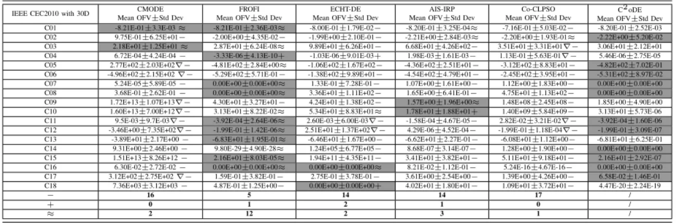
In terms of the 18 test functions with 30D from IEEE CEC2010, Tables VI, VII, and VIII record the average and standard deviation of objective function values, results of the multiple-problem Wilcoxon’s test, and results of the Friedman’s test, respectively. As shown in Table VI, C2oDE surpasses CMODE, FROFI, ECHT-DE, AIS-ISP, and Co-CLPSO on 16, five, 14, 14, and 17 test functions, respectively. However, the performance of FROFI, ECHT-DE, and AIS-ISP is better than that of C2oDE on only one, two, and one test function, respectively. In particular, CMODE and Co-CLPSO cannot beat C2oDE even on one test function. Regarding the multiple-problem Wilcoxon’s test, C2_{oDE provides higher}_R+ values thanR−values in all cases. Moreover, thep-values are less than 0.1 in all cases and less than 0.05 in four cases, i.e., C2_{oDE versus CMODE, C}2_{oDE versus ECHT-DE, C}2_oDE versus AIS-IRP, and C2_{oDE versus Co-CLPSO. With respect} to the Friedman’s test, C2_{oDE ranks the first followed by} FROFI. In conclusion, C2_{oDE provides superior results on the} 18 test functions with 30D from IEEE CEC2010. Moreover, it seems that the advantage of C2oDE over the five competitors increases as the number of dimension increases.

To visualize the experimental results, the convergence graphs of C2oDE, FROFI, and CMODE were plotted on six

(10)

(a) C02 with 10D (b) C14 with 10D (c) C18 with 10D

(d) C02 with 30D (e) C14 with 30D (f) C18 with 30D Fig. 4. Convergence graphs of C2_{oDE, FROFI, and CMODE on six representative test functions from IEEE CEC2010.}

TABLE IX

EXPERIMENTAL RESULTS OFC2_O_DE_AND_C_O_DE_OVER₂₅_INDEPENDENT

RUNS ON36TEST FUNCTIONS FROMIEEE CEC2010

Instance 10D 30D

C2oDE Mean OFV±Std Dev

(feasible rate)

CoDE Mean OFV±Std Dev

(feasible rate)

CoDE Mean OFV±Std Dev

(feasible rate) C01 -7.44E-01±7.39E-03 -7.47E-01±1.88E-03≈ -8.20E-01±2.52E-03 -8.11E-01±1.69E-03− C02 -2.26E+00±4.64E-02 -1.34E+00±7.11E-01− -2.22E+00±5.20E-02 9.21E-01±1.06E+00− C03 0.00E+00±0.00E+00 3.55E-01±1.78E+00− 3.06E+01±2.12E+01 (0%)− C04 -1.00E-05±0.00E+00 -6.74E-06±2.63E-06− 5.46E-06±2.75E-05 (0%)− C05 -4.84E+02±3.48E-13 (36%)− -4.82E+02±7.02E-01 (0%)− C06 -5.79E+02±6.17E-02 (28%)− -5.31E+02±8.97E-02 (0%)− C07 0.00E+00±0.00E+00 7.37E-25±2.41E-24− 0.00E+00±0.00E+00 1.49E+01±2.51E+00− C08 7.30E+00±5.18E+00 1.71E+00±3.99E+00+ 0.00E+00±0.00E+00 6.56E+01±4.65E+01− C09 5.17E+00±5.19E+01 4.13E-24±5.38E-24+ 1.85E+00±4.90E+00 (24%)− C10 3.67E+01±1.38E+01 2.17E+01±2.13E+01+ 3.13E+01±5.73E-06 (4%)− C11 -1.52E-03±4.89E-13 -1.52E-03±1.39E-07≈ -3.92E-04±1.60E-06 (0%)− C12 -7.63E+01±1.22E+02 (84%)− -1.99E-01±3.09E-07 (4%)− C13 -6.84E+01±2.77E-14 -6.84E+01±1.83E-02≈ -6.81E+01±6.25E-01 -5.92E+01±8.71E-01− C14 0.00E+00±0.00E+00 5.09E-25±8.48E-25− 0.00E+00±0.00E+00 2.12E+01±1.93E+00− C15 3.71E+00±1.65E-01 2.06E+00±1.86E+00+ 2.16E+01±2.92E-07 4.39E+12±2.64E+12− C16 0.00E+00±0.00E+00 0.00E+00±0.00E+00≈ 0.00E+00±0.00E+00 3.39E-05±2.09E-05− C17 1.61E-02±8.04E-02 1.17E-04±1.86E+00+ 6.58E-02±1.46E-01 (60%)− C18 0.00E+00±0.00E+00 2.50E+01±1.10E+02− 4.47E-20±2.24E-19 1.19E+04±8.70E+03−

− / 9 / 18

+ / 5 / 0

≈ / 4 / 0

representative test functions from IEEE CEC2010, i.e., C02 with 10D, C14 with 10D, C18 with 10D, C02 with 30D, C14 with 30D, and C18 with 30D. Since the source codes of ECHT-DE, AIS-IRP, and Co-CLPSO cannot be available, their convergence graphs are not provided. Fig. 4 depicts the evolution of the mean of the best feasible objective function value. As shown in Fig. 4, C2oDE converges faster than CMODE on all these six test functions. In addition, C2oDE shows faster convergence speed than FROFI on all these six test functions except for C14 with 30D. In terms of C14 with 30D, C2oDE and FROFI have similar convergence speed.

According to the above comprehensive experiments on two benchmark test sets, C2_{oDE exhibits very competitive} performance when tackling COPs.

D. Comparing C2oDE with the Original CoDE for Con-strained Optimization

The aim of this subsection is to ascertain whether the original CoDE designed for global optimization can be directly

applied to solve COPs. To this end, the search algorithm of C2oDE was replaced with the original CoDE. Subsequently, the 36 test functions from IEEE CEC2010 were used to produce the experimental results for CoDE. The average and standard deviation of objective function values over 25 runs are summarized in Table IX. It is noteworthy that the feasible rate, i.e., percentage of runs where at least one feasible solution is found, is recorded if an algorithm fails to consistently provide feasible solutions over all 25 runs. In addition, the Wilcoxon’s rank sum test at a 0.05 significance level was executed to compare C2_{oDE with CoDE. The cell with the smaller average} objective function value is highlighted in gray.

As shown in Table IX, overall, CoDE performs better than, similar to, and worse than C2oDE on five, four, and 27 test functions, respectively. More importantly, CoDE cannot consistently find feasible solutions in 12 cases. Therefore, the above comparison indicates that the original CoDE without any modifications is not a good choice as the search algorithm for constrained optimization, which verifies the motivation of this paper.

E. Contribution of the Feasibility Rule and theεConstrained Method

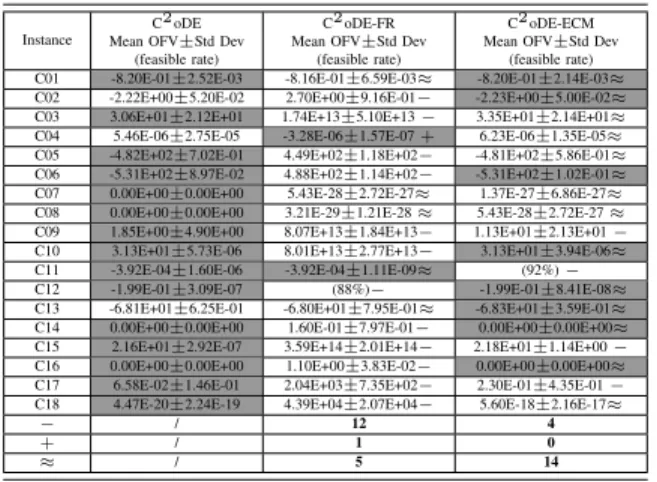
In this paper, our constraint-handing technique includes two phases. Moreover, the feasibility rule and the ε constrained method are used for the first and second phases, respectively. In order to identify their main contribution, two C2oDE vari-ants, i.e., C2oDE-FR and C2oDE-ECM, were implemented. To be specific, in C2oDE-FR, the feasibility rule was utilized in both phases while in C2_{oDE-ECM, the} _ε _constrained method was utilized in both phases. The 18 test functions with 30D from IEEE CEC2010 were employed to produce the experimental results.

The average and standard deviation of objective function values over 25 runs, and the feasible rate are summarized

(11)

TABLE X

EXPERIMENTALRESULTS OFC2_O_{DE, C}2_O_DE-FR,_AND_C2_O_DE-ECM

OVER25 INDEPENDENTRUNS ON18 TESTFUNCTIONS WITH30D FROM

IEEE CEC2010

Instance

C2oDE

Mean OFV±Std Dev

(feasible rate)

C2oDE-FR

Mean OFV±Std Dev

(feasible rate)

C2oDE-ECM

Mean OFV±Std Dev

(feasible rate)

C01 -8.20E-01±2.52E-03 -8.16E-01±6.59E-03≈ -8.20E-01±2.14E-03≈

C02 -2.22E+00±5.20E-02 2.70E+00±9.16E-01− -2.23E+00±5.00E-02≈

C03 3.06E+01±2.12E+01 1.74E+13±5.10E+13− 3.35E+01±2.14E+01≈

C04 5.46E-06±2.75E-05 -3.28E-06±1.57E-07+ 6.23E-06±1.35E-05≈

C05 -4.82E+02±7.02E-01 4.49E+02±1.18E+02− -4.81E+02±5.86E-01≈

C06 -5.31E+02±8.97E-02 4.88E+02±1.14E+02− -5.31E+02±1.02E-01≈

C07 0.00E+00±0.00E+00 5.43E-28±2.72E-27≈ 1.37E-27±6.86E-27≈

C08 0.00E+00±0.00E+00 3.21E-29±1.21E-28≈ 5.43E-28±2.72E-27≈

C09 1.85E+00±4.90E+00 8.07E+13±1.84E+13− 1.13E+01±2.13E+01−

C10 3.13E+01±5.73E-06 8.01E+13±2.77E+13− 3.13E+01±3.94E-06≈

C11 -3.92E-04±1.60E-06 -3.92E-04±1.11E-09≈ (92%)−

C12 -1.99E-01±3.09E-07 (88%)− -1.99E-01±8.41E-08≈

C13 -6.81E+01±6.25E-01 -6.80E+01±7.95E-01≈ -6.83E+01±3.59E-01≈

C14 0.00E+00±0.00E+00 1.60E-01±7.97E-01− 0.00E+00±0.00E+00≈

C15 2.16E+01±2.92E-07 3.59E+14±2.01E+14− 2.18E+01±1.14E+00−

C16 0.00E+00±0.00E+00 1.10E+00±3.83E-02− 0.00E+00±0.00E+00≈

C17 6.58E-02±1.46E-01 2.04E+03±7.35E+02− 2.30E-01±4.35E-01−

C18 4.47E-20±2.24E-19 4.39E+04±2.07E+04− 5.60E-18±2.16E-17≈

− / 12 4

+ / 1 0

≈ / 5 14

in Table X. Besides, the Wilcoxon’s rank sum test at a 0.05 significance level was applied to compare C2_{oDE with each} of C2_{oDE-FR and C}2_{oDE-ECM. If a method obtains the} smallest average objective function value on a test function, the corresponding experimental results are highlighted in gray. As shown in Table X, C2_{oDE outperforms C}2_{oDE-FR and} C2_{oDE-ECM on 12 and four test functions, respectively. In} contrast, C2oDE-FR and C2oDE-ECM cannot perform better than C2oDE on more than one test function.

Therefore, the experimental results reveal the contribution of the feasibility rule and the ε constrained method for the first and second phases, respectively.

F. Investigation on How to Select the Best Individual

In the search algorithm of C2_{oDE, the individual with the} least degree of constraint violation is chosen as the “best” individual in the modified DE/rand-to-best/1/bin while the individual with the best objective function value is selected as the “best” individual in DE/current-to-best/1/bin. In this sub-section, we empirically investigated how to select the “best” individual. To this end, three C2oDE variants, i.e., C2 oDE-Exc, C2oDE-Obj, and C2oDE-Const, were implemented. In C2oDE-Exc, the manners of selecting the “best” individu-al in the modified DE/rand-to-best/1/bin and DE/current-to-best/1/bin were exchanged. Specifically, the “best” individual in the modified DE/rand-to-best/1/bin was selected in terms of the objective function value while the “best” individual in the DE/current-to-best/1/bin was selected according to the degree of constraint violation. In C2_{oDE-Obj, both the modified} DE/rand-to-best/1/bin and DE/current-to-best/1/bin selected the “best” individual according to the objective function value. On the contrary, both of them selected the “best” individual in terms of the degree of constraint violation in C2_oDE-Const. The 18 test functions with 30D from IEEE CEC2010 were adopted for comparison.

The average and standard deviation of objective function values over 25 runs, and the feasible rate are summarized in Table XI. Also, the Wilcoxon’s rank sum test at a 0.05

TABLE XI

EXPERIMENTALRESULTS OFC2_O_{DE, C}2_O_DE-E_XC_{, C}2_O_DE-O_BJ_,_AND

C2_O_DE-C_{ONST OVER}_{25 I}_NDEPENDENT_R_{UNS ON}_{18 T}_EST_F_UNCTIONS

WITH30D FROMIEEE CEC2010

Instance

(feasible rate)

C2oDE-Exc Mean OFV±Std Dev

(feasible rate)

C2oDE-Obj Mean OFV±Std Dev

(feasible rate)

C2oDE-Const Mean OFV±Std Dev

(feasible rate) C01 -8.20E-01±2.52E-03 -8.20E-01±2.51E-03≈ -8.18E-01±3.65E-03≈ -8.20E-01±2.67E-03≈ C02 -2.22E+00±5.20E-02 -2.11E+00±8.73E-02≈ -2.20E+00±7.06E-02≈ -2.07E+00±1.07E-01− C03 3.06E+01±2.12E+01 3.05E+01±6.49E+00≈ 3.67E+01±2.63E+01≈ 2.87E+01±1.57E-09≈ C04 5.46E-06±2.75E-05 2.32E-04±6.13E-04− 2.89E-05±1.19E-05− 1.79E-03±1.96E-03− C05 -4.82E+02±7.02E-01 -3.77E+02±2.10E+02− -4.82E+02±5.24E-01≈ -2.63E+02±2.60E+02− C06 -5.31E+02±8.97E-02 -5.30E+02±2.51E-02≈ -5.31E+02±2.50E-02≈ -5.29E+02±1.23E+00≈ C07 0.00E+00±0.00E+00 2.49E-24±3.75E-24− 0.00E+00±0.00E+00≈ 25.21E-20±1.85E-19− C08 0.00E+00±0.00E+00 1.84E-20±5.22E-20− 5.43E-28±2.72E-27≈ 2.46E-16±9.08E-16− C09 1.85E+00±4.90E+00 1.42E+01±2.37E+01− 7.87E+00±1.88E+01− 2.65E+01±2.95E+01− C10 3.13E+01±5.73E-06 3.13E+01±2.63E-06≈ 3.13E+01±3.82E-06≈ 3.13E+01±4.70E-06≈ C11 -3.92E-04±1.60E-06 -3.92E-04±1.11E-09≈ (84%)− -3.92E-04±2.35E-09≈ C12 -1.99E-01±3.09E-07 (80%)− -1.99E-01±1.81E-08≈ -1.99E-01±4.96E-06≈ C13 -6.81E+01±6.25E-01 -6.77E+01±5.30E-01≈ -6.82E+01±5.38E-01≈ -6.69E+01±7.63E-01≈ C14 0.00E+00±0.00E+00 9.74E-22±1.65E-21− 0.00E+00±0.00E+00≈ 8.38E-18±1.96E-17− C15 2.16E+01±2.92E-07 2.16E+01±1.10E-07≈ 2.16E+01±2.79E-07≈ 2.16E+01±1.78E-07≈ C16 0.00E+00±0.00E+00 0.00E+00±0.00E+00≈ 0.00E+00±0.00E+00≈ 0.00E+00±0.00E+00≈ C17 6.58E-02±1.46E-01 1.90E-01±4.62E-01− 4.62E-01±1.69E+00− (96%)− C18 4.47E-20±2.24E-19 6.48E-20±2.28E-19≈ 6.72E-04±3.35E-03− 4.99E-05±2.49E-04−

− / 8 5 9

+ / 0 0 0

≈ / 10 13 9

TABLE XII

EXPERIMENTALRESULTS OFC2_O_DE_AND_C2_O_DE-W_O_R_OVER₂₅

INDEPENDENTRUNS ONTHREETESTFUNCTIONS WITH10D (C11WITH

10D, C12WITH10D,ANDC17WITH10D)ANDONETESTFUNCTION WITH30D (C12WITH30D)FROMIEEE CEC2010

Instance

(feasible rate)

C2oDE-WoR Mean OFV±Std Dev

(feasible rate) C11 with 10D -1.52E-03±4.89E-13 (4%) C12 with 10D -7.63E+01±1.22E+02 (0%) C17 with 10D 1.61E-02±8.04E-02 (76%) C12 with 30D -1.99E-01±3.09E-07 (92%)

significance level was used to compare C2_{oDE with each of} C2_{oDE-Exc, C}2_{oDE-Obj, and C}2_{oDE-Const. The} experimen-tal results with the smallest average objective function value among the four compared methods are highlighted in gray on each test function. As shown in Table XI, C2_{oDE surpasses} C2_{oDE-Exc, C}2_{oDE-Obj, and C}2_{oDE-Const on eight, five,} and nine test functions, respectively. However, C2oDE-Exc, C2oDE-Obj, and C2oDE-Const cannot beat C2oDE on any test function.

The above experimental results suggest that the manner of selecting the “best” individual in C2_{oDE is reasonable.}

G. Effectiveness of the Restart Scheme

In order to analyze the effectiveness of the proposed restart scheme, a method called C2_{oDE-WoR was implemented} by removing the restart scheme from C2_{oDE. The 36 test} functions from IEEE CEC2010 were selected for experiments. The average and standard deviation of objective function values resulting from C2oDE-WoR were computed. The exper-imental results of those test functions, for which C2oDE and C2oDE-WoR do not have significant performance difference based on the Wilcoxon’s rank sum test at a 0.05 significance level, were omitted. As a result, Table XII provides the experimental results for four test functions. In Table XII, the feasible rate is also provided if a method cannot attain feasible solutions consistently.

As shown in Table XII, the restart scheme plays a very important role in the performance of C11 with 10D, C12 with