Copyright by Jakob Infuehr
The Dissertation Committee for Jakob Infuehr
certifies that this is the approved version of the following dissertation:
Relative Performance Evaluation, Analysts,
Convertible Debt
Committee:
Volker Laux, Supervisor
Andres Almazan Michael Clement Aysa Dordzhieva Ronghuo Zheng
Relative Performance Evaluation, Analysts,
Convertible Debt
by
Jakob Infuehr
Dissertation
Presented to the Faculty of the Graduate School of The University of Texas at Austin
in Partial Fulfillment of the Requirements
for the Degree of
Doctor of Philosophy
The University of Texas at Austin
Acknowledgments
I would like to thank my dissertation committee: Andres Almazan, Michael Clement, Aysa Dordzhieva, Volker Laux (chair), and Ronghuo Zheng. Also, I appreciate helpful comments from Prasart Jongjaroenkamol, seminar par-ticipants at The University of Texas at Austin, the University of Alberta, the University of Southern Denmark, the Leibniz University of Hanover, the Management Accounting Section Midyear Meeting, and the Tenth Accounting Research Workshop.
Volker Laux, my adviser throughout the Ph.D. program, was of invalu-able help. He gave me the freedom and guidance to pursue and achieve my research goals.
I am also indebted to Antonis Kartapanis. His support and friendship the last five years made my life here in Austin a great time. Similarly, Colin Koutney and Xinyu Zhang gave me so much joy. They were always there for me when I needed them most.
Kristen Valentine, Brian Monsen, Zheng Leitter, Ben Van Landuyt, Shannon Garavaglia, Yue Wang, Dan Rimkus, Ryan Hess, Ryan Ballestero, and Skylar DeTure all were very kind to me.
your continuous support and love. I try to make you proud as best as I can.
Jakob Infuehr
The University of Texas at Austin May 2019
Abstract
Relative Performance Evaluation, Analysts,
Convertible Debt
Jakob Infuehr, Ph.D.
The University of Texas at Austin, 2019
Supervisor: Volker Laux
This dissertation addresses several research questions. First, I show that rel-ative performance evaluation incentivizes more earnings management. The optimal contract will depend less on a correlated benchmark, if it is easier for the manager to misreport performance. Thus, the model predicts that firms with strong internal controls and good auditors are more likely to use RPE. Second, I show that a higher analyst following can lead to more or less earnings management, depending on the skewness of the earnings distribution. Analysts try to minimize their forecast error, while managers try to beat the average forecast target. Thus, the actors’ actions influence each other. Third,
I study the effects of accounting conservatism on the use of convertible debt. In the model, firms use these financial contracts to separate themselves from bad firms, while trying to minimize costs of financial distress. A very aggres-sive accounting system helps good firms separate and avoid financial distress, because this makes a low signal more informative and less likely, causing in-vestors not to convert to equity after such a signal.
Table of Contents
List of Tables xii
List of Figures xiii
Chapter 1 Relative Performance Evaluation and Earnings
Man-agement 1 1.1 Introduction . . . 1 1.2 Related Literature . . . 5 1.3 Model . . . 8 1.4 No Manipulation . . . 11 1.5 Manipulation . . . 14 1.5.1 Exogenous Contract . . . 14 1.5.2 Endogenous Contract . . . 17 1.5.3 Comparative Statics . . . 21 1.5.4 A manipulated benchmark . . . 23 1.5.5 Renegotiation . . . 24 1.6 Conclusion . . . 26
Chapter 2 Meet or beat analysts’ forecasts, skewness, earnings
management, and investment choice 28
2.1 Introduction . . . 28 2.2 Related Literature . . . 33 2.3 Model . . . 37 2.4 Earnings management . . . 39 2.4.1 Many Analysts . . . 40 2.4.2 One Analyst . . . 41 2.4.3 Comparative Statics . . . 46 2.4.4 Discussion of Results . . . 48 2.5 Investment . . . 50
2.6 Manipulation and Investment . . . 54
2.7 Conclusion . . . 58
Chapter 3 Accounting Conservatism and Convertible Debt 60 3.1 Introduction . . . 60 3.2 Related Literature . . . 66 3.3 Model . . . 69 3.4 Perfect Signal . . . 72 3.5 Imperfect Signal . . . 75 3.6 Miscellaneous . . . 82 3.6.1 Comparative Statics . . . 82 3.6.2 Short-Term Debt . . . 84
3.7 Conclusion . . . 87
Appendix A Proofs for Chapter 1 89
Appendix B Proofs for Chapter 2 102
Appendix C Proofs for Chapter 3 107
List of Tables
List of Figures
1.1 Optimal Compensation . . . 20
2.1 Manager’s Reporting Strategy . . . 39
2.2 Effect of a Change in Analyst’s Forecast on Manager’s Report-ing Strategy . . . 42
2.3 Mean-preserving spread and Median . . . 47
2.4 Manipulation and Investment . . . 57
Chapter 1
Relative Performance
Evaluation and Earnings
Management
1.1
Introduction
Incentivizing executives to work hard has been studied extensively in the lit-erature. Holmstrom (1982) was one of the first to show that using the per-formance of the competition in determining compensation can be desirable if there are common shocks that influence output. Filtering this additional noise gives a better understanding of the executive’s effort and reduces the risk imposed on the worker. Positive covariance among firms’ performances seems to be descriptive of the real world, where industry-wide and
economy-wide events regularly affect multiple firms at once. Hence, one would expect a widespread use of relative performance evaluation (RPE). Yet, empirical re-search has found only modest use. Bannister and Newman (2003) and Gong, Li, and Shin (2011) find that less than half of firms use RPE.1 A good example
of this is the oil industry. In 2007, at the height of oil prices, executives re-ceived (compared to other industries) disproportionately high pay raises, four times as high as the average (Herbst 2008). A similar correlation was observed in 2015. When oil prices plummeted, so did the compensation of many ex-ecutives. Median compensation fell, while it rose in other industries (Olsen 2016).
Bertrand and Mullainathan (2001) provide one potential explanation for the lack of RPE. They find that ”better governed firms pay less for luck,” and conclude that this is consistent with the hypothesis that CEOs have power over their boards and essentially set their own pay. In contrast, I show that the fact that weaker corporate governance is associated with less RPE use can also occur in an optimal contracting setting, in which the manager has no power over the compensation committee. An important feature in my model is that the CEO can manipulate the performance measure on which her compensation is based. I find that the optimal contract will make less use of RPE if the CEO can more easily misreport the performance measure.
The intuition for this result is driven by a nonlinearity in the optimal contract. Consistent with empirical evidence (Bannister and Newman 2003,
Garvey and Milbourn 2006), in my model the manager receives a large re-ward for outperforming the benchmark, but her compensation only decreases slightly for underperforming it. This causes two effects, both of which are disadvantages of RPE.
First, the nonlinearity creates a difference in ex-post manipulation centives. When the manager performs similar to the benchmark, ex-post in-centives to manipulate will be higher, while they are lower when she underper-forms the benchmark. If the manager’s performance were uncorrelated with the benchmark, then these forces would offset, and ex-ante expected manip-ulation would be unchanged. However, because the manager’s performance and the benchmark are positively correlated, the chance that the manager performs similar to the benchmark increases. Hence, she is more likely to be in a scenario when she has high incentives to manipulate, and less likely to be in a situation when she has low incentives to manipulate. Without RPE, a contract could still be nonlinear. Yet, the lack of correlation due to the absence of a benchmark means that the manager is not more likely to be in a situation when her manipulation incentives are strong. Therefore, RPE in expectation incentivizes a higher level of manipulation compared with a lack of RPE use.
The second effect working against RPE is about the observability of the benchmark. The manager has to commit to her effort decision early in the year, well before the benchmark is realized. Ideally, she would prefer to work hard when the benchmark is easier to beat, and shirk when it is harder.
However, she does not have to commit to an earnings management decision until very late in the fiscal year, possibly even after the fiscal year already ended. Real earnings management decisions such as accelerating next year’s sales (by giving discounts) or delaying R&D spending by a month can be made in December; and accrual-based earnings management can be executed even in January, when many major (discretionary) accounting decisions have to be made. At that point, she will have already observed the outcome of shocks, such as changes in economic conditions, industry demand, etc. Thus, the manager can condition the manipulation level on the realization of the benchmark. With nonlinear RPE, her manipulation decision will depend on her performance relative to the benchmark. This makes manipulation more efficient for the agent, hence reducing the incentive effect to actually work hard. Benchmark-independent pay does not have this disadvantage, because the informational advantage is useless to the agent. Her manipulation decision would be independent of economic conditions in that case.
The firm of course anticipates the two above described effects and proac-tively responds by reducing the weight of relative compensation in the contract structure. It trades off the benefit of using the more informative signal with the benefit of reducing incentives to manipulate. This result can explain why so few firms find it optimal to use RPE, despite the contrarian theoretical prediction. The result also leads to the empirical prediction that RPE will be used more in firms with better corporate governance, tighter accounting standards, etc. that limit the CEO’s manipulation potential.2
The remaining paper is organized as follows. Section 1.2 discusses re-lated literature, section 1.3 describes the model, section 1.4 analyzes the sce-nario without earnings management, section 1.5 discusses the main results and also explores some comparative statics, and section 1.6 concludes. All proofs are in appendix A.
1.2
Related Literature
Relative performance evaluation (RPE) has received some attention in the academic literature. One of the earliest papers is Holmstrom (1982). He showed that the optimal compensation scheme of an agent depends on his performance alone if and only if his performance is independent from anyone else’s. In the case of independence, no information about the agent’s actions can be learned from comparing his output with another one. It would only add noise and thus be detrimental in the case of risk-aversion because the additional risk that is imposed on the agent has to be compensated. However, with dependence, some information is embedded in the performance of others and this can be used to more precisely incentivize effort. Under some conditions, a weighted average of all performances and the agent’s output is a sufficient statistic.
Holmstrom’s results did not specify how the weighted average should
capturing the pay-setting process. My prediction can use e.g. distance between firm head-quarters and the auditor’s office (Choi et al. 2012, Kubick et al. 2017), while powerful CEOs can be measured using CEO tenure, CEO-board duality, etc.
be used in the compensation scheme. This is an important question that was addressed in subsequent research. Banker and Datar (1989) find necessary and sufficient conditions when a linear aggregation of signals is optimal. More specifically, using profit is only optimal, when revenue and costs are equally intense (sensitivity times precision) signals. Celentani and Loveira (2006) find that ”if the marginal return of effort depends on the aggregate state, optimal contracts are not monotonically decreasing in the performance benchmark” and claim that this may explain the lack of RPE use in the business world. Fleckinger (2012) generalizes these results by not imposing any restrictions on the correlation of outcomes. His results predict that RPE is most effective when covariance is constant and positive.
RPE has, of course, also been studied in the empirical literature. Early papers (e.g. Janakiraman, Lambert, and Larcker 1992, Aggarwal and Samwick 1999) had to resort to indirect tests and did not find positive results. SEC rule changes since then allowed the application of direct methods (e.g. Bannister and Newman 2003, Gong et al. 2011) and results indicated that about a quarter of all firms use RPE. Bannister and Newman (2003) also find, as well as Garvey and Milbourn (2006), that firms use one-sided RPE, executives get rewarded for outperforming the peer-group, but do not get punished for underperformance. This result is consistent with the theoretical results of Celentani and Loveira (2006) and Feriozzi (2011). I also find this in my setting, although the reason is different. In my model, the assumption of limited liability leads to one-sided RPE.
Prior analytical research has proposed solutions for the relative perfor-mance evaluation puzzle. Dye (1992) finds that the agent’s option to choose among different projects can negatively affect RPE. Gopalan et al. (2010) study a similar idea. The agent will pick a project (or industry) where his skill is relatively high (compared to the peers in that industry), but may be low in absolute terms. This is not in favor of the principal, who cares about absolute profit, not relative one. Another paper is Dikolli et al. (2011), who hypothesize that the empirical literature may have committed Type II errors by summing peer-performance differently compared to boards (selecting more, fewer or different peers). This could lead to a lower estimate on the number of firms that use RPE in compensation contracts.3
The only published paper thus far to study the intersection of RPE and earnings management is Bagnoli and Watts (2000). However, their paper does not endogenize the agent’s compensation structure and therefore does not examine the effect of earnings management on the use of RPE, key aspects of my paper. There is also no moral hazard problem. A recent working paper by Balakrishnan, Lin, and Sivaramakrishnan (2016) studies ranking systems and its susceptibility to performance manipulation. This paper, though, is more closely related to the tournament theory literature, rather than the RPE literature.
3Other papers that discuss the RPE puzzle include Fershtman et al. (2003) and DeMarzo
1.3
Model
I consider a one-shot game with a risk-neutral principal and a risk-neutral agent.
Timing: There are two dates,t ={0,1}. At date 0, the principal hires an agent to be in charge of a project and offers her a compensation contract. After signing the contract, the agent can exert costly effort that increases the probability of success. At date 1, the outcome of a correlated benchmark is publicly observed. The agent privately learns whether her project succeeded or failed, R ∈ {S, F}.4 Then, she issues a potentially manipulated report.
Based on the report and the benchmark, the agent is paid and the game ends.
Effort: The agent makes a binary effort decision after being hired:
e ∈ {el, eh} (shirk or work). The probability of success, pe = Pr(R =S|e), is strictly greater whene =eh is chosen, i.e., ph > pl. Effort imposes a disutility on the agent,k(e), and without loss of generality, I assume thatk(eh) = cand
k(el) = 0. Furthermore, to avoid trivial solutions, I assume that the principal always wants to incentivize high effort.
Benchmark: There is an observable and contractible benchmarkZ ∈ {G, B} (good or bad). The benchmark Z could be the S&P 500, which could be low or high (in this binary model) or other quantitative indices of economic conditions. Commodity prices are another option.5
4Unobservable outcome might occur, if the project is long-term, but the agent needs to
be compensated before the end of the project.
5A somewhat more endogenous choice would be the average performance of a peer group.
R\Z B G
F (1−pe+γ)(1−q) (1−pe−γ)q
S (pe−γ)(1−q) (pe+γ)q Table 1.1: Joint Probabilities
The probability that the benchmark is good is q. A pair of results can take four values, Y ∈ {SG, SB, F G, F B}. Let the probability of the good benchmark be independent of the agent’s effort decision, Pr(Z =G|e) = Pr(Z =G) = q. However, this does not imply that the probabilities of project success and benchmark are independent. There is a positive covariance γ, which alters the conditional success probabilities such that Pr(R = S|Z =
G) =pe+γ and Pr(R=S|Z =B) = pe−γ. Letγ be small enough such that all probabilities are between zero and one. This leads to the joint probabilities for the four possible outcomes displayed in table 1.1.
These probabilities capture, in the simplest form possible, the character of positive correlation. The probability that the benchmark is good and the agent successful increases. For example, when the economy is doing well, a CEO’s projects are more likely to succeed. The assumption of a constant covariance imposes a restriction on the model to keep the focus on the effects of earnings management, and the exposition simple.6
Report: At date 1, the agent observes the outcome of her project and the benchmark with certainty. She will then issue a report to the principal,
model. The situation I want to analyze focuses on a CEO, who does not have a comparable coworker within the same company.
r∈ {rS, rF}. Let the combination of the report and the observable benchmark be denoted by y∈ {ySG, ySB, yF G, yF B}. The agent can take an unobservable, manipulative action m ∈ [0,1] to issue a favorable report, even though the project has failed. mis the probability that a failed project will be misreported as a success, i.e. m = Pr(r = rS|R = F). The agent would never misreport good news because in the optimal contract compensation is higher when the report is better. Generally, the manipulation level will take two different values, mG and mB, depending on the benchmark, good and bad respectively. The cost of manipulation is gm2/2, where g is an exogenous parameter
that captures how easily reports can be manipulated.7 For example, better
auditors, tighter accounting standards, and a vigilant board would cause g to be higher. Furthermore, I assume that g > g ≡ 2c
ph−pl to guarantee an interior solution, i.e. m <1, in equilibrium.8
Contracting: The agent is risk-neutral and thus maximizing her ex-pected wage,E[wy]. The only variable that is available for contracting, is the combination of the report and the benchmark, y. Thus, the agent is offered a contract w = {wSG, wSB, wF G, wF B} that specifies four state-dependent pay-ments. For example, the agent receives wSB when she reports a success and
7One could assume thatgdepends on the realization of the benchmark. When conditions
are bad, auditors may expect more manipulation, thus auditing more. The results of the paper are qualitatively unchanged, as long as the two differentg’s are close to each other.
8These assumptions about the manager’s reporting have been used extensively in prior
literature with binary models and earnings management (e.g. Dutta and Gigler 2002, Jong-jaroenkamol and Laux 2017).
the benchmark is bad, y = ySB. The agent is protected by limited liability, that is w ≥ 0 for each element of the vector. The reservation utility is set to zero. The participation constraint will not bind in equilibrium, and first-best cannot be achieved.
An incentive scheme exhibits RPE, when ∆w≡(wSB−wSG)>0, joint performance evaluation (JPE), when ∆w < 0, and independent performance evaluation (IPE), when ∆w = 0. The greater the difference, the greater the extent of RPE/JPE. wF G and wF B are not part of this definition because in the optimal solution these payments are zero.
1.4
No Manipulation
The no-manipulation setting is a special case of the general model described above, when g → ∞ and therefore m = 0. This case demonstrates the main advantage of RPE.
The principal minimizes expected compensation cost
min
wSB,wSG,wF G,wF B E[wy] = (ph−γ)(1−q)wSB+ (ph+γ)qwSG+
subject to the agent’s incentive constraint
(ph−γ)(1−q)wSB+ (ph+γ)qwSG+ (1−ph−γ)qwF G+
+ (1−ph+γ)(1−q)wF B −c≥(pl+γ)qwSG+ (pl−γ)(1−q)wSB+ + (1−pl−γ)qwF G+ (1−pl+γ)(1−q)wF B, (1.2)
and the limited liability constraint
wSG, wSB, wF G, wF B ≥0. (1.3)
Solving this problem leads to the following proposition.
Proposition 1.1When earnings management is not possible (g → ∞), then the optimal contract satisfies
wSB > wSG =wF G =wF B = 0. (1.4)
It is optimal to set wF G =wF B = 0, because any positive payment for failure would only make it more difficult to provide incentives for the agent to work hard. The reason for wSB > wSG is a little more subtle. Holmstrom’s work (1979, 1982) shows that it is efficient to incentivize effort by linking pay to the signal that is most informative about effort. If an agent is successful, despite a low benchmark, then success is a very informative signal about the agent’s effort. However, high agent performance in the presence of a good benchmark is a less informative signal about effort. Formally, this can be
expressed with likelihood ratios: Pr(y=ySB|e=eh) Pr(y=ySB|e=el) > Pr(y=ySG|e=eh) Pr(y=ySG|e=el) or (ph−γ)(1−q) (pl−γ)(1−q) > (ph+γ)q (pl+γ)q . (1.5) These likelihood ratios measure how strongly y = ySB and y = yySG, respectively, signal that the agent chose high rather than low effort. A high likelihood ratio speaks for high effort; a value of one would indicate that noth-ing new is learned from the signal (Hart and Holmstrom 1987). The inequality in (1.5) shows thaty=ySB (agent is successful and benchmark is bad) is more informative than y=ySG.
However, if one were to introduce risk-aversion, then there is a trade-off. A large spread between wSB and wSG imposes a risk on the agent, which has to be compensated in the form of a risk premium. The principal would have to strike a balance between the risk premium and putting more weight on the more informative signal. More risk-averse agents would be offered a contract with less RPE, and agents that have a project with higher covariance would be subject to more RPE (to filter out more correlated noise).
The results in the paper do not rely on risk aversion and the model therefore assumes risk neutrality, to keep the intuition simple. However, all results are robust to the assumption about the curvature of the agent’s utility function. Imposing greater risk is a well-known problem associated with RPE. The focus of the paper, though, is on another problem, and risk aversion is thus ignored.
1.5
Manipulation
Consider now the setting of main interest, in which earnings management is possible, that is g <∞.
1.5.1
Exogenous Contract
I first analyze the manager’s optimal level of manipulation for any exoge-nous contract which satisfies the incentive constraint with equality. I set
wF B = wF G = 0, as these payments do not incentivize high effort. Taking the derivative of the agent’s utility function (A.13) with respect to mB and
mG, respectively, yields mB = wSB g and mG = wSG g . (1.6)
Manipulation depends on the outcome of the benchmark, Z, because the agent can observe Z before the manipulation decision. In contrast, effort cannot be conditioned on Z because the manager only observes Z after the effort decision.
The expected manipulation level E[m], in general terms, is
E[m] = (1−pe+γ)(1−q)mB+ (1−pe−γ)qmG. (1.7)
For the expected manipulation level, the following proposition can be obtained.
Proposition 1.2 Expected manipulation level E[m] is always higher for RPE (wSB > wSG) than for benchmark-independent compensation (wSB =
wSG). E[m] is minimized, when JPE is used. The minimal manipulation inducing contract is characterized by an interior solution wSG > wSB > 0, when earnings management is easy (g < gT), and by the corner solutionwSG >
wSB = 0, when g > gT.9
Solving for the contract that satisfies the incentive constraint (A.16) with equality, plugging all results into (1.7), taking the derivative of E[m] with respect to wSB, and substituting wSG back in for simplicity, gives the following result:10 dE[m] dwSB = 1 g(1−ph+γ)(1−q)− 1 g(1−ph−γ) g −wSB g−wSG (1−q). (1.8)
The first summand in (1.8) is the direct effect of an increase in wSB on
mB. The manager will manipulate more when the benchmark is low (mB), if the bonus payment he receives when he is successful and the benchmark is low, wSB, is higher. The second summand in (1.8) is the indirect effect of an accompanied decrease in wSG and hence mG. Several insights can be gained from (1.8). First, when wSB > wSG (RPE), then the derivative in (1.8) is positive, i.e. an increase in RPE always increases expected manipulation.
9g
T is defined in the appendix, equation (A.20).
10Note that in a contract that satisfies the incentive constraint with equality, w SB and
wSG are negatively related. When one payment increases, the other can be lowered. Thus,
This result can be traced back to the positive correlation between the manager’s performance and the benchmark, as well as the nonlinearity of the contract. Nonlinear RPE creates incentives to manipulate more when the benchmark is bad, because wSB −wF B > wSG −wF G. Manipulation allows the manager to report that she outperformed the benchmark and collect a big bonus. This scenario is more likely to occur when positive correlation is at play because the agent is likely to perform similar to the benchmark. Additionally, the optimal contract creates lower incentives to manipulate when the bench-mark is good. Manipulation only allows the CEO to hide her underperfor-mance relative to the benchmark, and avoid a small penalty (equivalently: re-ceive a small bonus). This case is less likely to occur due to correlation because the agent’s performance is less likely to deviate from the benchmark. Since these forces flip when joint performance evaluation (JPE) is used,wSB < wSG, expected manipulation is lower with JPE.
The fact that expected manipulation can have an interior minimum, when manipulation is cheap, is driven by another key force in the model. That force concerns the observability of the benchmark. If it is observable before the manipulation decision, then the manipulation level, when the benchmark is good, will differ from the level, when it is bad (as long as wSB 6= wSG). If it were unobservable, then by construction the agent would have to choose
mB =mG. The loss of a degree of freedom for the agent means that she will receive a lower utility to the benefit of the principal. He can pay out the larger bonus less often because the agent is less efficient in her manipulation decision.
This leads to the following proposition.
Proposition 1.3 If compensation depends on the benchmark (wSB 6=
wSG), then the agent’s utility is higher when she can observe the benchmark. This result is a drawback for both RPE and JPE, and explains why expected manipulation need not be monotonically decreasing as JPE usage increases.
This second effect also is true due to the asymmetric contract induced by limited liability. When the agent submits a low report, then compensation is zero, no matter what. If compensation were symmetric, such that wSB −
wSG = wF B − wF G, then manipulation incentives would be independent of the benchmark. This is an important point to emphasize. In a LEN model, the linear restriction imposed on the contract makes it symmetric and thus this effect would not be present. The asymmetric contract can arise in many situations, depending for example on how effort affects covariance or limited liability (as is the case in this paper), and is consistent with evidence from archival studies (e.g. Bannister and Newman 2003).
1.5.2
Endogenous Contract
I now turn to the endogenous contract setting when manipulation is possible. It is essentially the patterns described in Proposition 1.2 and Proposition 1.3 that lead to the following proposition describing the optimal contract.
Proposition 1.4 The optimal contract has the following characteris-tics:
(i)wSB > wSG = 0 (max RPE) when g ∈[g∗,∞),11 (ii) wSB > wSG >0 (RPE) when g ∈(bg, g
∗),
(iii) wSG =wSB (IPE) when g =bg ≡
8c
3(ph−pl),
(iv) wSG > wSB >0 (JPE) when g ∈(g,bg),
(v) wSG−wSB →0 (asymptotically IPE) when g →g ≡ ph2−cpl.
The possibility of report manipulation creates a trade-off in the RPE usage. On the one hand, RPE is beneficial due to the positive correlation (as seen in the benchmark scenario). On the other hand, RPE incentivizes higher manipulation. As a result, when the use of RPE indeed causes a significantly higher manipulation level, then the principal will be more inclined to abstain from benchmarking compensation. In fact, this effect can be high enough, such that the principal actually prefers joint performance evaluation (JPE), i.e. wSB < wSG, for some levels of g that are close enough to g. This means that the agent actually earns a higher wage, when the competition was also successful. The fact that the agent can observe the benchmark before her manipulation decision is also a disadvantage for JPE and thus favors inde-pendent compensation. However, the other key intuition that worked against RPE, works in favor of JPE. The agent wants to report a success while the benchmark is high. This outcome is more likely due to the positive corre-lation, thus effort is more likely to achieve the desired result. On the other hand, the lack of correlation for manipulation does not help it, and thus, it is not as efficient in reaching the agent’s preferred outcome. Of course, JPE runs
counter to using the most informative signal, but when the manager can easily manipulate (g close to g), then its advantages can outweigh the drawbacks. Atg =bg, the forces balance exactly, and independent performance evaluation is optimal.
Part (v) of Proposition 1.4 follows because the principal has to take ma-nipulation into account, and a very uneven compensation structure incentivizes heavy manipulation because the agent can wait and observe the outcome of the benchmark. For example, for wSB > 0 and wSG = 0, she would manipu-late heavily when the benchmark is low and not at all when the benchmark is high. Given the convex manipulation cost function, the agent has to be compensated for this manipulation (or else she shirks) with a very high payoff that can be avoided by smoothing compensation across states. As a result, in addition to the forces described in the previous section, RPE now has an ad-ditional disadvantage when the agent can wait and observe the outcome of the benchmark. The agent is now in a better position to efficiently exploit RPE because she will not waste her manipulation effort when it is not as beneficial to her.
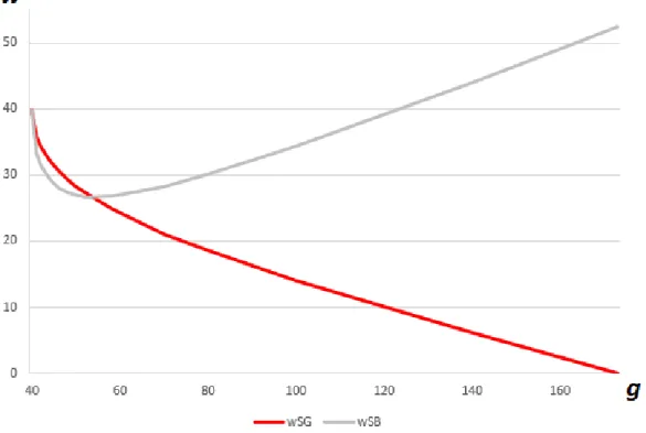
Figure 1.1 illustrates an example of the above described observations.12
In the figure, g∗ ≈ 173. It is the point where wSG hits the x-axis. For g ≥ g∗ (not pictured), when manipulation is very costly, the agent only receives money if she reports success and the benchmark is low. The graph shows the main relationship. As earnings management becomes less costly
12The example uses the parametersp
Figure 1.1: Optimal Compensation
(moving from right to left on the graph), the firm has to reduce the importance of the benchmark by decreasing the difference between the two wage payments
wSB and wSG. At the very left end of the chart (when g approaches g = 40), incentivizing the agent to work hard becomes tough enough that both wage payments have to increase to accomplish this feat. For g < g, no solution exists. Threre is also a small range, g ∈ (40,1603 ), where joint performance evaluation is optimal, i.e. wSG > wSB. At g = 1603 , the two wage payments are identical.
1.5.3
Comparative Statics
I now turn the analysis to some comparative statics. Less RPE is used when either the range ”max RPE” in part (i) of Proposition 4 shrinks (i.e. g∗
increases) or the range ”RPE” in part (ii) of Proposition 4 gets smaller (i.e. bg
increases).
Corrolary 1.1 RPE is used less as (i) covariance (γ) decreases,
(ii) probability of success (ph) decreases, and (iii) cost of effort (c) increases.
A change in correlation has two effects. First, when correlation in-creases, then this increases the advantage of RPE as seen in the proof of the no manipulation scenario (see appendix). The likelihood ratios diverge and it is increasingly easier to incentivize effort using RPE. Second, an increase in correlation increases the difference in manipulation levels that RPE and in-dependent compensation cause. While earnings management does not change if benchmark-independent pay is used, it does with RPE. This is again owed to the fact that an increase in correlation makes it harder to outperform the competition by regular means, which is why the promised compensation has to increase. This increased compensation in turn causes the increase in ma-nipulation. However, the second effect is lower than the main effect on the informativeness of the signal.
An increase inph is beneficial for RPE because it alleviates the incentive problem. The agent is more likely to succeed if he puts in the effort, and effort
matters more because pl is kept constant, increasing (ph − pl). Thus, the principal does not need to offer as much compensation which of course also decreases the manipulation incentives. And as already established, a principal that is less concerned about manipulation, will use RPE more heavily. The effect ofccan best be understood, when the ratiogc is viewed as the relative cost of effort in relation to the cost of manipulation. Characteristics like optimal use of RPE and equilibrium manipulation level are unaffected, as long as gc stays constant. It is thus not surprising that an increase inc causes a proportional increase in g∗.
Corollary 1.2 As manipulation becomes more difficult (g increases), (i) expected manipulation goes down,
(ii) expected wage decreases, (iii) the agent’s utility decreases.
Part (i) of the corollary can be explained as follows. When manipulation is more costly to the agent, holding everything else equal, he will manipulate less. A counteracting force here is the fact that with less manipulation, the principal will use more RPE. However, this force is weaker than the first one. If the principal would increase RPE too much and cause more, not less, manipu-lation, then he would again suffer too much from the negative consequences of RPE, and compensation would not be optimal. Hence, RPE will only increase slowly and expected manipulation will decrease.
Part (ii) of the corollary follows because less manipulation makes it eas-ier to incentivize effort. As noted above, the ratio cg is important as the agent
always weighs her options to achieve the desired result. So when manipulation is harder, the bonus necessary to induce effort declines.
Part (iii) follows because even though expected wage decreases, it is not immediately obvious that this implies that the agent’s utility also decreases. After all, manipulation decreases and consequently also the cost of manipula-tion. Why is it not possible that the second effect outweighs the first one? It is instructive to note that the agent can freely choose the manipulation level. When g decreases, she has the option to maintain the original manipulation levels, mB and mG. This implies that she could keep the manipulation cost down while simply enjoying the increased wage. The only reason why the agent increases manipulation, is because it increases her overall utility. There is no reason why the agent would intentionally hurt herself and cause her utility to decline.
1.5.4
A manipulated benchmark
Thus far I have assumed that the benchmark is completely exogenous. How-ever, a reasonable argument can be made that executives at the other com-panies can manage earnings as well. In this subsection I analyze how the optimal contract and the agent’s behavior changes in response to a change in
q, the probability that the benchmark is good. While this does not endoge-nize the benchmark completely, it is a reasonable approximation in situations when each individual firm is only a small part of the peer-group. When that is the case, each individual manager’s actions will have negligible effects on other
firms’ decisions. A higherqcan be a stand-in for other firms also manipulating their earnings, thus causing the benchmark to be higher more frequently.
The most direct and obvious effect of an increase inq(when other firms manipulate more) is that it becomes harder to outperform the benchmark. The probability that the agent is successful while the benchmark is low de-creases. This in turn requires an increased bonus, if one wants to use RPE, to compensate for the decreased likelihood of achieving the bonus. That bigger bonus, however, incentivizes more manipulation, and the board then uses less RPE.
Corollary 1.3 RPE is used less (g∗ increases) as the probability of a high benchmark, q, increases.
1.5.5
Renegotiation
One aspect that often receives some attention in the literature is renegotiation. On the one hand, allowing for renegotiation undermines commitment. On the other hand, it can also be used to incorporate new information into the contract that was not available at the beginning.
To illustrate the former point, imagine that in the present model rene-gotiation is possible after the agent has made her effort decision. If the agent is risk-averse, then renegotiation can be mutually beneficial, because the agent bears some risk that can be completely transferred to the principal. The agent receives a flat wage, regardless of outcome. Unfortunately, this can and will be anticipated by the agent. Realizing that, ultimately, compensation will be
independent of outcome, and the agent has no incentive to work.
Illustrating the latter point is possible if renegotiation is possible after the agent privately observes the outcome of her project. At first, it might seem that the principal is in a bad spot to renegotiate because the agent has an informational advantage about the project outcome. However, this does not really matter because if the agent was successful, then she will not accept any new contract that would reduce the pay that she is guaranteed to receive. After failure, renegotiation can prevent earnings management because the agent will receive a flat wage. This time, if the principal has all the bargaining power, it does not affect ex-ante effort incentives. This is because expected ex-ante utilities, depending on outcome, do not change. The agent is still interested in achieving success because his pay will be higher in that case. However, because earnings management will not occur, this can be anticipated by the principal and will therefore affect the initial contract that is offered to the agent. The contract that would be offered without renegotiation would still satisfy the agent’s incentive constraint. The key difference is that the principal can save the agent’s manipulation cost via renegotation. Hence, a contract that would lead to more manipulation, if renegotation were not available, can be offered. Thus, the optimal contract will feature a heavier reliance on RPE, since RPE again would incentivize more earnings management.
Proposition 1.5 If renegotiation is possible after the agent observed the outcome and the principal has all the bargaining power, then there exists a new threshold gn∗ such that the optimal contract sets wSB >0 and wSG = 0
if and only if g ≥ gn∗. The new threshold is lower than the old one, gn∗ < g∗, i.e. more RPE is used. Additionally, JPE is never optimal.
1.6
Conclusion
This paper analyzes the effect of earnings management on the profitability of relative performance evaluation (RPE). When the manager cannot misreport, using RRP is optimal because it filters industry-wide shocks and allows for a more accurate measure of the CEO’s performance. High firm performance when the competition failed is a more informative signal than good perfor-mance when others succeeded, too. This insight would predict that RPE should be widespread in the business world, given that positive correlations are common. However, empirical research shows that this is not the case. I show that one potential explanation for this can be earnings management. Manipulation makes it easier for a manager to report success, while the com-petitors fail. This is the case because manipulation success is less correlated than real outcomes. Whether an auditor for company A demands an adjust-ment will depend less on whether another auditor demanded an adjustadjust-ment for company B. Additionally, when the manager can observe the benchmark before her earnings management decision, then RPE increases manipulation incentives even further because the agent will manipulate more when it is more advantageous to her. This gives the CEO an efficient way to boost her expected compensation and thus makes it harder to incentivize hard work.
nipulate and will switch to a compensation scheme that depends less on the competition in an effort to curb manipulation. Hence, the firm trades off the benefit of using the most informative signal with the drawback of incentiviz-ing manipulation. This result can explain why RPE is not as heavily used as predicted. For some companies, the benefit of RPE will not be big enough compared to its disadvantage.
Chapter 2
Meet or beat analysts’ forecasts,
skewness, earnings management,
and investment choice
2.1
Introduction
Analysts, in their role as information intermediaries, affect firms directly and indirectly in many ways. One of these is corporate governance. Yu (2008) and Chen et al. (2015) have found that a higher analyst coverage improves corporate governance, first and foremost by reducing earnings management. This finding lends support to the monitoring hypothesis: analysts study fi-nancial statements thoroughly, take part in conference calls with top level executives, and increase attention due to the dissemination of information.
Contrary to these results, there is recent research that finds negative conse-quences of increased analyst coverage. He and Tian (2013) find that firms with more analysts are less innovative, and Huang et al. (2017) show that more analyst coverage can cause firms to meet the forecast target more of-ten (which implies more, not less, manipulation). These results are taken as support for the pressure theory, which claims that analysts create pressure on managers to beat the forecast target. This theory is somewhat in conflict with the monitoring theory. However, there is another channel that indirectly affects manipulation decisions. Managers benefit from meeting or beating the analyst forecast target (Bartov et al. 2002) and hence make discretionary ac-counting choices to accomplish just that (e.g. Matsumoto 2002, Brown 2001). In this paper, I show that the number of analysts following a firm affects this channel. Hence, the observed empirical patterns can be explained, even when there is no analyst monitoring or pressure at all.
Specifically, I consider a model in which managers will manipulate earn-ings to just meet the average analyst forecast, if actual earnearn-ings are close enough to the target. I call this the ”manipulation range” and it shows in a histogram as a discontinuity gap. Analysts, on the other hand, try to mini-mize the forecast error between their (individual) forecasts and reported earn-ings (actual earnearn-ings are unobservable). Hence, managers are influenced by analysts’ forecasts, and analysts are influenced by managers’ choice of manip-ulation. I analyze two scenarios: when there are many analysts, and when there is only one covering the firm.1 In the former case, each analyst takes the
anticipated reported earnings distribution as given, and tries to minimize his or her forecast error accordingly. An equilibrium will form, when the analysts’ forecasts induce a reporting strategy by the manager, such that no analyst can change his forecast without increasing the forecast error.
This equilibrium will change, if there is only one analyst issuing an earn-ings forecast. Now, the lone analyst anticipates that a change in his forecast also changes the reported earnings distribution. That creates an incentive to decrease the forecast (compared to the equilibrium desribed above). If the reported earnings distribution wouldn’t change, then a small decrease in the forecast would not increase the forecast error by much (the first derivative of the forecast error at the optimum is zero). Also, if actual earnings fall in a range, where the manager would manipulate to the target either way, then this also does not affect the error. The change in error will occur on the edges of the manipulation range, especially the low end. When the manager would not manipulate in the original equilibrium because earnings were a little too far away from the target, he would manipulate now with the lowered target. This decreases the forecast error for this specific earnings realization to zero. On the high end, when actual earnings are just below or above the target, the change is negligible, because either way the forecast error will be small. In less technical words, the manipulation range is advantageous to the analyst because it reduces his forecast error. By reducing the forecast, the manager will manipulate slightly lower earnings that used to be farther away from the
forecast target.
The effect of a lower forecast target on the average accounting manip-ulation depends on the shape of the earnings distribution. When there are many analysts, then the forecast that minimizes the squared error is the mean of reported earnings (or median for absolute error, Gu and Wu 2003). When there is only one analyst, a lower forecast causes more manipulation if the earnings distribution (probability density function) at the mean is decreasing. The manipulation range shifts left, and thus actual earnings are more likely to fall into that range. This is the case when the earnings distribution is posi-tively skewed as then the mode of the distribution is lower than the mean. The reverse is true for a left-skewed distribution. Actual earnings are less likely to fall into the manipulation range when the number of analysts covering the firm decreases.
This result shows that analyst following can impact earnings manage-ment, even when analysts do not monitor the firm, when earnings are skewed. Earnings skewness is an overlooked attribute in prior studies (Yu 2008, Chen et al. 2015) on this topic. Gu and Wu (2003) find that the median skewness is about zero, but there is ”large cross-sectional variation in earnings skewness.” Hence, it seems plausible that average skewness in other studies could be pos-itive or negative, depending on the specific sample that is used. Therefore, I propose that skewness should be a control variable in future research to clearly identify the forces driving the relationship.
changing the reporting strategy, but also by changing the underlying actual earnings distribution via investments. A key difference between the two is that investment decisions are usually long-term, and thus have to be made well in advance of analysts issuing their forecasts. Therefore, analysts will take the investment decision as given, regardless of the number of analysts, and no dif-fering equilibria emerge. The manager still cares about beating the average forecast as often as possible. If the earnings distribution is symmetric, then there is no incentive to deviate from first-best, because first-best gives the manager a 50% chance to beat the forecast, which he cannot improve upon. However, when the distribution is skewed, and if analysts forecast the median, then a deviation from first-best is optimal for the executive. First-best invest-ment will maximize the expected value, while the manager cares about the median. If median and mean are different (due to skewness), then he has an incentive to improve the median, even when this comes at the expense of a decrease in the mean. Depending on his opportunity set, this could lead to a preference for right-skewed earnings distributions.
The above result shows that it can be perfectly rational for a manager to prefer a more right-skewed earnings distribution, as observed by Schneider and Spalt (2016). They find that ”capital expenditure is increasing in the expected skewness of segment returns.” However, they attribute this result to the fact that managers use gut feel, which causes them to subjectively assess probabilities, overweighting low probability events, as predicted by prospect theory (Kahnemann and Tversky 1979). Instead, I show that managers’ desire
to beat the analyst forecast can be the driving force behind this observed pattern.
Finally, I show that the interaction of investment and reporting deci-sions incentivizes the manager to underinvest (i.e. reduce variance) in order to improve the probability that earnings management allows him to beat the target. Thus, for left-skewed distributions, the possibility of earnings manage-ment can improve investmanage-ment efficiency. The incentive to increase variance in order to improve the median, and the incentive to decrease variance to improve the efficiency of accounting manipulation can cancel each other out.
The remaining paper is organized as follows. Section 2.2 discusses re-lated literature, section 2.3 describes the model, section 2.4 analyzes the sce-nario when earnings management is possible, section 2.5 discusses the case when the manager’s investment choice is endogenous, section 2.6 examines the interaction between manipulation and investment, and section 2.7 concludes. All proofs are in appendix B.
2.2
Related Literature
There are several streams of literature relevant for this paper. The first one is the literatue dealing with managers’ incentives to meet or beat the analyst forecast target. Brown (2001) finds that during the 1990s, median forecast errors have shifted from small negative to small positive, indicating an in-creased incentive to meet or beat the average forecast. Additionally, the share of small positive surprises increased over time, and is more pronounced in
growth firms. Brown and Caylor (2005) confirm this trend, and further show that since the mid-1990s the managerial tendency to avoid negative earnings surprises is stronger than the one to avoid negative earnings or earnings de-creases. They attribute this pattern to ”increased media coverage given to analyst forecasts, more analyst following, more firms covered by analysts, and temporal increases in both the accuracy and precision of analyst forecasts.” Furthermore, Armstrong et al. (2017) find that the analysts’ external EPS goal is more important to managers than internal incentive plan EPS goals.
Additional research tried to pinpoint the exact source of managerial in-centives. Mutsunaga and Park (2001) examine the CEO’s annual discretionary bonus (allocated from a bonus pool) and find that the bonus is negatively af-fected if the consensus analyst forecast is not met for at least two quarters of the year, while there is no significant effect for loss quarters. This reduc-tion in bonus pay is in addireduc-tion to the tradireduc-tional linear pay-for-performance sensitivity. Bartov et al. (2002) study the stock market’s reaction to barely beating the analysts’ earnings expectations. They find that there exists a mar-ket premium for beating expectations, even ”after controlling for the earnings forecast error for that period.” This premium exists, even when beating ex-pectations was probably achieved via earnings management. Furthermore, the premium does not fade over a longer time window, indicating that ”investors rationally react to the earnings surprises.” Finally, Matsumoto (2002) looks at firm characteristics that are associated with an increased likelihood to beat expectations. These include ”firms with higher transient institutional
owner-ship, greater reliance on implicit claims with their stakeholders, and higher value-relevance of earning.” These characteristics may by related to increased incentives for managers to beat expectations. Similar to other studies, Mat-sumoto finds that managers, in addition to accounting manipulation, guide analysts’ expectations downward, to increase chances of beating these.
The second stream of literature is the analyst following literature. There are of course many firm characteristics that determine analyst following (e.g. Bhushan 1989: size, institutional ownership, return volatility, market return, business complexity), but the one particularly related to this paper is about earnings management. Previts et al. (1994) in their qualitative study find that analysts are aware of ”adjustments of conservative, discretionary reserves, allowances, and off-balance-sheet assets” and noted that analysts seemed to like these adjustments. This observation is consistent with my theoretical model, which finds that analysts benefit from earnings management due to the reduction in forecast error.
More relevant than the determinants of analyst coverage, which are ex-ogenous in my model, are studies about the effect of analyst following on firms. Quite a few papers find positive effects of analyst coverage on firms, such as market value (Chung and Jo 1996), less earnings management (Yu 2008), less excess CEO compensation, and pay-for-performance sensitivity (Chen et al. 2015). All of these studies attribute these positive effects to the analyst mon-itoring hypothesis, which states that analysts apply pressure on management by increasing investor attention and disseminating information. On the other
hand, there is recent research that finds negative consequences of increased analyst coverage. He and Tian (2013) find that firms with more analysts are less innovative, and Huang et al. (2017) show that more analyst coverage can cause firms to meet the forecast target more often. These results are taken as support for the pressure theory, which claims that analysts create pressure on managers to beat the forecast target. This theory is somewhat in conflict with the monitoring theory. Contrary to these theories, I posit and show an-alytically that the effects can also possibly be explained without the need for monitoring or pressure.
The final stream of literature is related to earnings distribution skew-ness. Skewness causes mean and median to diverge, which is relevant when making an assumption about analysts’ utility function. Gu and Wu (2003) and Basu and Markov (2004) make the case that analysts minimize their absolute forecast error, and hence forecast the median. Lastly, Schneider and Spalt (2016) study the consequences of earnings skewness on investment decisions. They find that CEOs overinvest, when earnings distributions are right-skewed, consistent with the long-shot bias proposed by the prospect theory (Kahne-man and Tversky 1979). In this paper, I show that this observed pattern can be rationally explained by management’s desire to outperform earnings expectations.
2.3
Model
I consider a one-period game with three dates, a firm manager and one or more analysts.
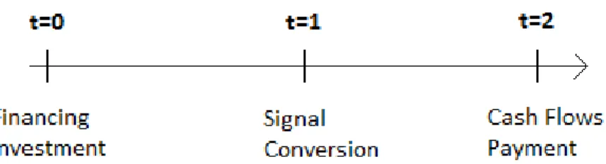
Timing: There are three dates,t ={−1,0,1}. Att =−1, the manager invests k into a project that yields a return at t = 1. At t = 0, each analyst simultaneously issues a forecast, predicting firm earnings. At t = 1, earnings realize, but are not observable to anyone but the firm manager. Then, the manager issues a potentially manipulated report, each player receives their payoff, and the game ends.
Earnings and investment: At t = 1, unobservable earnings x are realized. The probability density function isf(x), the cumulative distribution function isF(x), the mean and variance depend on the investment, d2dkE2[x] <0,
there exists k=kF B, such that dEdk[x] = 0, V ar[x]>0 for all k, and dV ardk[x] >0 for all k. While the location and scale parameters of the distribution depend on investment, the shape parameters (skewness, kurtosis) do not, they are constant. For ease of exposition, I assume that the distribution is single-peaked. The assumptions about the earnings distribution capture the notion that any deviation from the optimal amount of risk, will decrease expected earnings. Also, I will examine both observable and unobservable investment.
Manager and report: I assume that the manager’s only incentive is to meet or beat the mean analyst earnings forecast z:
max
Z ∞
z
whereg(y) is the probability density function of reported earnings yas defined below.
The manipulation results change slightly, if the median forecast matters, and this will be addressed. The investment results are robust. If earnings x
are sufficiently close to the forecast z (0 < z−x < m) , then he will issue a manipulated report y, and otherwise issue an unmanipulated report:
y= z if z−m ≤x≤z x otherwise . (2.2)
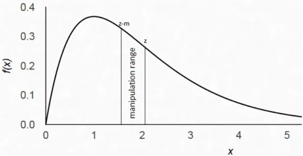
Also, I will refer to [z−m, z] as the ”manipulation range” because the manager will only manipulate if earnings fall within this range. The assump-tions above capture, in the simplest form possible, the empirically observed fact that managers have incentives to meet or beat the analysts’ forecast tar-get. Figure 2.1 illustrates a possible example.
Analysts: The analysts know the earnings distribution, f(x). Each analyst’s goal is to minimize the squared difference between his or her forecast and reported earnings, i.e. min
z E[(z−y)
2].They are all equally well-informed
and thus, in equilibrium, will all issue the same forecastz. These assumptions warrant some discussion. The key characteristic of the utility function is that the analyst suffers a loss that is increasing in the forecast error. Alternative specifications are possible, such as minimizing the absolute error or maximiz-ing expected reputation (if there were multiple analyst types). The results for investment depend on this assumption, and will receive further discussion
Figure 2.1: In this example, unmanipulated earnings x are distributed in the form of a Gamma distribution: f(x) ∼ Γ(2,1). The forecast is z = 2.05. The manipulation range width is m = 0.5. Thus, the manipulation range is [1.55,2.05]. For these values, the mean of reported earnings will be equal to the forecast, an equilibrium, when there are many analysts.
below. Additionally, there is no forecast dispersion in this model, because all analysts are equally well informed. This assumption simplifies the exposition, but does not affect any inferences.
2.4
Earnings management
In this section, I assume that investment is exogenously given, and normalize
E[x] = 0. Thus, the complete focus of this section is on the effects of earnings management. Furthermore, for mathematical convenience, I assume thatm is small compared toV ar[x], i.e. V arm[x] →0.
2.4.1
Many Analysts
In this subsection, I assume that there are infinitely many analysts. Each analyst’s effect on the average forecast target is negligible. As a result, every analyst takes the manager’s reporting strategy as given. The analysts minimize their squared error, which means that their forecast has to be the expected value of the reported earnings distribution:
z =E[y] = Z z−m −∞ xf(x)dx+z(F(z)−F(z−m)) + Z ∞ z xf(x)dx. (2.3)
The first and last summands are the unmanipulated reports, when earn-ings are either too far away from the target or higher than the target and no manipulation is necessary. The middle term represents reported earnings when actual earnings are just a hair below the average forecast. In that instance, the manager would manipulate the report to meet the forecast. Since reported earnings are higher than actual unobservable earnings by the amount of ma-nipulation, the above equation can also be written as:
z =E[y] =E[x] |{z} =0 + Z z z−m (z−x)f(x)dx. (2.4)
Thus, equation (2.4) shows expected manipulation, when there are many analysts. Note that they are evaluated based on the difference between their forecast andreported earnings. Analysts have to anticipate the manager’s expected amount of manipulation and adjust their forecasts upward
accord-of the reported earnings distribution influenced by the analysts’ forecasts has to match the analysts’ mean forecast. Only then will analysts not have any incentive to deviate from the equilibrium strategy. I do not need to solve for
z explicitly, since I am not interested in the location of z, but how z changes as the number of analysts changes.
2.4.2
One Analyst
I now analyze the situation, when there is only one analyst. The analyst will take the effect of his report on the reporting strategy of the manager into account, and due to this indirect effect, the forecast will deviate from the expected value of reported earnings. The analyst’s objective is as follows:
min
z E[(z−y)
2]. (2.5)
Since I only need to find out whether the forecast will be lower or higher than the one in the last section, it is sufficient to analyze the change in squared error at the expected value. At that value, the direct effect will be zero, because the derivative at an optimum is zero. Small deviations from an optimum do not matter much. Therefore, it will be the indirect effect via the change in the manager’s reporting strategy that determines the new equilibrium. Let the ”many analysts equilibrium forecast” bezm and the ”one analyst equilibrium forecast” bezo. Assume thatzo < zm (to be verified later). Then there are two ranges, where the reporting strategy changes: at the lower
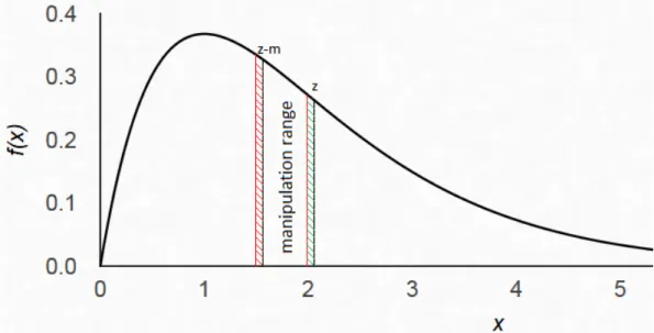
end of the manipulation range [zo−m, zm−m] and at the higher end of the manipulation range [zo, zm]. Figure 2.2 illustrates this.
Figure 2.2: This is the same distribution as in Figure 2.1: f(x) ∼ Γ(2,1). When there are few analysts, they will lower the forecast. The two important changes to the manager’s reporting strategy occur at the lower end of the manipulation range (region with red stripes) and at the higher end (region with green stripes). Changes in forecast error for the regions below the red striped one and above the green striped ones balance each other. Between the red and green region, the forecast error will be zero.
Thus, we can obtain the following formula for the change in squared error: E[(zo−y)2]−E[(zm−y)2] = Z zm zo (x−zo)2f(x)dx− Z zm−m zo−m (zm−x)2f(x)dx. (2.6) The first summand is the increase in error at the high end of the
manipulate to the target. With the lowered forecast, he no longer has to ma-nipulate when earnings fall into this range, and there will be a positive error. The second summand is the decrease in error at the low end of the manipula-tion range. With the lowered target, the manager will now manipulate to the target and the error is zero. Originally, earnings were too low at this point and the manager did not manipulate, leading to a positive error. One can see that the error in the first term will be close to zero because with a lower target, reported earnings are only a smidgen above the forecast. However, the error in the second term is positive because it is at leastm. Formally, using a first-order approximation approach shows that the first term approaches zero, while the second term is nonzero. Thus, the squared error is decreasing atzm, proving thatzo< zm is correct, which is summarized in the following lemma.
Lemma 2.1The fewer analysts follow a firm, whose forecasts are used as a target for the manager, the lower the forecast will be.
Intuitively, the manipulation range is beneficial to the analysts, because it eliminates the forecast error compeletely. If actual earnings fall into this range, then the manager manipulates to the forecast, and the error is zero. The analyst, if there are not too many following the same firm, can influence the manager’s reporting strategy and hence the location of the manipulation range. Naturally, he would like to eliminate bigger, rather than smaller, forecast errors. Essentially, the analyst lowers his forecast to allow the manager to manipulate to the target for lower earnings realizations than before.
is the median forecast, then there will be no change in equilibrium, when there are three or more analysts. This is because no single analyst can change the median by changing his forecast, when there are at least three analysts. Although, if one were to introduce forecast dispersion into the model, then each analyst, ex-ante, would have a N1 chance (N is number of analysts) of issuing the median forecast. Thus, each analyst would anticipate that a change in his forecast would matter in expectation by N1 of that change, and results would be the same as when the manager’s target is the mean forecast.
Now we can go back to equation (2.4) and evaluate how manipulation changes when the forecast decreases. The width of the manipulation range (m) and the amount of manipulation (z −x) are unchanged. However, the probability that manipulation occurs will be different. If the mean of the earn-ings distribution is on the downward sloping part (mean higher than mode), then a forecast decrease will increase the probability of manipulation. Vice versa, if the mean is on the upward sloping part of the distribution, then a forecast decrease will decrease the probability of manipulation. The mean of a distribution is higher than the mode, if it is right-skewed (or positively skewed) using the Pearson mode skewness. Formally, we can see the above intuition taking a derivate of equation (2.4) and applying the Leibniz rule:
d dz(
Z z
z−m
(z−x)f(x)dx) =F(z)−F(z−m)−mf(z−m). (2.7)
The remainder of the proof again uses first-order approximation. Thus, we can state the above result in the following proposition.
Proposition 2.1 A lower analyst following leads to more expected manipulation if the earnings distribution is right-skewed and vice versa.
The above result shows that the number of analysts covering a firm can influence that firm’s manager’s earnings management decisions, even when there is no monitoring occuring. Prior archival studies (Yu 2008, Chen et al. 2015) on this topic have attributed the relationship to the monitoring hypoth-esis without accounting for potential effects of skewness. Gu and Wu (2003) find that the median skewness is about zero, but there is ”large cross-sectional variation in earnings skewness.” Hence, it seems plausible that average skew-ness in other studies could be positive or negative, depending on the specific sample that is used. Therefore, I propose that skewness should be a control variable in future research to clearly identify the forces driving the relationship. In the model, analysts are completely rational. Yet, from an outsider’s perspective, it can appear as if a lone analyst does not minimize the forecast error, if one mistakenly assumes the manager’s reporting strategy is constant. Archival researchers can observe that expected value (or median for that mat-ter) of reported earnings and analyst forecast do not match when there are few analysts (Brown 1997, Lim 2001, Hong and Kacperczyk 2010). However, this bias is not real and perfectly reasonable from the analyst’s point of view. The analyst not only minimizes the error given the distribution, but also takes the indirect effect, by changing the manager’s manipulation strategy, into account.
2.4.3
Comparative Statics
The model allows for more insights to be gained about the effect of analyst coverage on accounting manipulation.
Corollary 2.1An increase in variance of the earnings distribution leads to
(i) less expected manipulation,
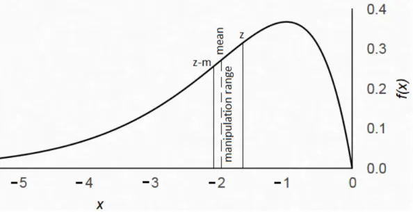
(ii) a decreased impact of a change in analyst following on manipulation. The first one follows from the fact that an increase in variance makes it less likely that actual earnings fall just below the forecast target. Most of the time, earnings will either be high enough such that manipulation is not necessary, or low enough such that too much manipulation would be required (more than the manager is comfortable with). Intuition for (ii) is as fol-lows: Since manipulation is less likely to occur, analysts will be less concerned about a change in their forecasts affecting the manager’s reporting strategy. This effect causes forecasts to increase and approach the ”many analysts equi-librium”. Another effect happens, if analysts forecast the median, because a mean-preserving spread changes the median, as long as the distribution is skewed. For example, for a right-skewed distribution, an increase in variance leads to a decrease in the median (see Figure 2.3).
Corollary 2.2 When the earnings distribution becomes more skewed (deviates more from zero skewness), then a change in analyst following causes a larger change in earnings management.
Figure 2.3: The black line is the same probability density function as in the previous figures: f(x)∼ Γ(2,1). the grey line is f(x+ 0.5)∼ Γ(2,0.75). For both distributions, E[x] = 2. However, the median of the grey distribution with less variance (1.76) is higher than the median of the black distribution (1.68), illustrating the manager’s incentives to decrease variance, when the distribution is right-skewed.
in analyst following on manipulation, if the distribution is not skewed at all. There will still be an effect on the average forecast, but a change in the forecast does not lead to a change in expected manipulation because the probability density function is flat around the mean (and median). As skewness deviates more from zero, this does not persist and the probability of manipulation changes with a change in the forecast (i.e. the first derivative of the probability density function is nonzero).
increase in analysts’ forecasts.
Analysts try to forecast reported earnings, not actual earnings. If ma-nipulation is easier fo