Macro variables and the components of stock returns.

Durham Research Online

24 March 2015

Version of attached le:

Accepted Version

Peer-review status of attached le:

Peer-reviewed

Citation for published item:

Maio, P. and Philip, D. (2015) 'Macro variables and the components of stock returns.', Journal of empirical nance., 33 . pp. 287-308.

Further information on publisher's website: http://dx.doi.org/10.1016/j.jempn.2015.03.004

Publisher's copyright statement:

NOTICE: this is the author's version of a work that was accepted for publication in Journal of Empirical Finance. Changes resulting from the publishing process, such as peer review, editing, corrections, structural formatting, and other quality control mechanisms may not be reected in this document. Changes may have been made to this work since it was submitted for publication. A denitive version was subsequently published in Journal of Empirical Finance, 33, September 2015, 10.1016/j.jempn.2015.03.004.

Additional information:

Use policy

The full-text may be used and/or reproduced, and given to third parties in any format or medium, without prior permission or charge, for personal research or study, educational, or not-for-prot purposes provided that:

• a full bibliographic reference is made to the original source

• alinkis made to the metadata record in DRO

• the full-text is not changed in any way

The full-text must not be sold in any format or medium without the formal permission of the copyright holders. Please consult thefull DRO policyfor further details.

Durham University Library, Stockton Road, Durham DH1 3LY, United Kingdom Tel : +44 (0)191 334 3042 | Fax : +44 (0)191 334 2971

Macro variables and the components of stock returns

Paulo Maio

Dennis Philip

First version: January 2012

This version: January 2014

1_{Hanken School of Economics, P.O. Box 479, 00101 Helsinki, Finland. E-mail:}

paulof-maio@gmail.com.

2_{Durham Business School, Mill Hill Lane, Durham DH1 3LB, UK. E-mail:}

den-nis.philip@durham.ac.uk.

3_{We thank Aurobindo Ghosh, Jun Ma, Jesper Rangvid, Richard Roll, Hongyu Song, and}

partic-ipants at the 2012 Arne Ryde Workshop, the 2012 SKBI Conference organized by Singapore Man-agement University, the 2012 INQUIRE UK Workshop, and the 2013 FMA Meeting in Chicago for helpful comments. We are grateful to Kenneth French and Robert Shiller for making data available on their webpages. Previous versions circulated with the titles “Do macro variables drive stock and bond returns?” and “Do macro variables drive stock returns?”. Any remaining errors are our own.

Abstract

We conduct a decomposition for the stock market return by incorporating the information from 124 macro variables. Using factor analysis, we estimate six common factors and run a VAR containing these factors and financial variables like the market dividend yield and the T-bill rate. Including the macro factors does not have a significant impact in the estimation of the components of aggregate (excess) stock returns—cash-flow, discount-rate, and interest rate news. Using the macro factors in the computation of cash-flow and discount-rate news does not significantly improve the fit of a two-factor ICAPM for the cross-section of stock returns.

Keywords: asset pricing; macroeconomy and stock returns; return decomposition; stock return predictability; discount-rate news; cash-flow news; Intertemporal CAPM; cross-section of stock returns; factor analysis

1

Introduction

What drives stock returns? Since the seminal work of Campbell and Shiller (1988) and Campbell (1991) there has been growing interest in connecting the variation in realized stock returns with shocks to future discount rates (discount-rate news) and cash flows (cash-flow news). The bulk of the analysis has been in conducting variance decompositions for stock returns, based on short-run vector autoregressions (VAR), which enable us to assess if the variation in realized stock returns is associated with discount-rate news or cash-flow news. An incomplete list of papers that conduct a return decomposition for aggregate stock returns includes Campbell and Ammer (1993), Patelis (1997), Campbell and Vuolteenaho (2004), Bernanke and Kuttner (2005), Sadka (2007), Larrain and Yogo (2008), Chen and Zhao (2009),Garret and Priestley (2012), andMaio (2013c). Other studies compute variance decompositions at the portfolio or individual stock level (e.g., Vuolteenaho (2002), Callen and Segal (2004),Callen, Hope, and Segal (2005), Hecht and Vuolteenaho (2006), Eisdorfer (2007), and Maio (2013a)).

In this paper, we conduct a variance decomposition for stock returns by incorporating the information associated with a large macroeconomic panel data set. One of the common criticisms associated with the VAR identification of the components of stock returns (based on a small number of state variables) is the bias caused by the specification error incurred when estimating discount-rate news. This translates into a misspecification of cash-flow news, which represents the “residual” of the return decomposition.1 _{This “missing predictor”}

problem is less likely to be relevant if we incorporate the information from a large group of variables to forecast stock returns and thus identify more properly discount-rate news. In fact, investors make decisions to invest in stocks based on information from a bounded, but potentially large, set of signalling variables. As stated before, if we erroneously exclude some of these variables, we will induce measurement errors in estimating cash-flow and discount-rate news. Since we cannot observe which macro variables are indeed the relevant state

variables, we include a large panel of macro information into our analysis. Moreover, this analysis enables us to check whether macro variables convey relevant information to forecast stock returns in addition to the variables usually employed in the predictability and return decomposition literatures—aggregate financial ratios (such as the dividend yield or earnings yield), bond yield spreads (such as the slope of the yield curve or the credit risk spread), or short-term interest rates. Therefore, the goal of this paper is to investigate whether there is missing macro information that is relevant when conducting return decompositions for the stock market.

We estimate six common macroeconomic factors using the asymptotic principal compo-nent analysis developed by Connor and Korajczyk (1986) and widely implemented for large macroeconomic panels (see, for example, Stock and Watson (2002a, 2002b)). These six fac-tors summarize the information from a panel of 124 macro variables from 1964:01 to 2010:09, which can be broadly classified into different categories: output and income; employment and labor force; housing; manufacturing, inventories and sales; money and credit; interest rates and bond yields; foreign exchange; and price indices.

We next estimate a first-order VAR containing the six macro factors, the aggregate stock return, the aggregate dividend growth, and the market dividend yield (d−p). This VAR specification is used to identify the components of the market return—discount-rate and cash-flow news. We use two alternative identification schemes. First, the benchmark procedure, which is typically used in the literature, consists of directly estimating discount-rate news and obtaining cash-flow news as the residual implied from the return decomposition. In the second procedure, we directly estimate cash-flow news and get discount-rate news as the residual component of the stock market return. We estimate the variance decomposition for the stock market return based on the benchmark VAR and a restricted VAR that excludes the macro factors, that is, it does not incorporate the information from the large macro panel set. The results show that the inclusion of macro factors, in addition tod−p, does not add significant information in estimating the components of aggregate stock returns, that is,

the contribution of each component for the variance of stock returns is basically the same whether we include or not the macro factors.

Since most of the related literature focuses on excess returns, we also analyze the impact of the macro variables on the components of excess stock returns by using a VAR specification that includes both the excess log stock return and the log interest rate. Overall, the results show that the macro factors play a relatively marginal role for the variance decompositions of the excess market return. Thus, the relative importance of the components of excess stock returns (cash-flow, discount-rate, and interest-rate news) does not change significantly by including the macro factors in a VAR that already contains the aggregate dividend yield and the T-bill rate. Therefore, such results suggest that these two financial state variables already incorporate most of the relevant information to identify the components of the equity premium.

One implication of these results is that the usual practice followed in the literature of defining a VAR with a limited number of state variables, borrowed from the predictability literature, does not seem to miss relevant information. Specifically, these results also indicate that if there are missing variables in the return decompositions for stock (excess) returns, those “missing” variables are not correlated with the large macroeconomic information set considered in this paper. Another way to interpret these results is that the macro variables do not add enough forecasting power (enough to change the relative importance of the stock return components) to a VAR that already contains the market dividend yield, the short-term interest rate (as well as lagged excess returns and dividend growth) in terms of predicting aggregate (excess) stock returns, dividend growth, or interest rates.

We also analyze the implications of using the macro factors in the estimation of the excess stock return components for the cross-section of stock returns. We use the time-series of cash-flow and discount-rate news to test the two-factor Intertemporal CAPM (ICAPM) fromCampbell and Vuolteenaho (2004). The objective is to assess whether the macro factors have an influence on the explanatory power of the model on the cross-section of stock returns.

The results indicate that using macro factors to identify the components of the excess stock market return does not improve significantly the explanatory power of the Campbell and Vuolteenaho (2004) two-factor model in pricing the 25 size/book-to-market portfolios.

Apart from the return decomposition literature mentioned above, this paper is related with previous work that uses macro factors, which summarize the information from a large data set of macro variables, to forecast stock returns (e.g.,Ludvigson and Ng (2007) orBai (2010)). The key difference relative to these papers is that we assess the impact of the macro factors in the estimation of the components of stock returns, rather than focusing only on return predictability. Our work is also related with a broader literature that focuses on the effect of macro variables on stock prices (e.g., McQueen and Roley (1993), Hess and Lee (1999),Flannery and Protopapadakis (2002),Boyd, Hu, and Jagannathan (2005),Bernanke and Kuttner (2005), Baele, Bekaert, and Inghelbrecht (2010), among others). Finally, the paper is also related with part of the asset pricing literature that derives and tests versions or extensions of the Campbell (1993) ICAPM (e.g., Campbell (1996), Chen (2003), Guo (2006), Khan (2008), Bianchi (2011), Botshekan, Kraeussl, and Lucas (2012), Campbell, Giglio, Polk, and Turley (2012), Maio and Santa-Clara (2012), Campbell, Giglio, and Polk (2013), Maio (2013c, 2013d), among others).

The paper proceeds as follows. In Section 2, we estimate the common macro factors. Section 3 provides a variance decomposition for the stock market return. In Section 4, we compute a variance decomposition for the equity premium. Section 5 analyzes the implica-tions for estimating a version of the ICAPM. Finally, Section 6concludes.

2

Macro variables and estimation of common factors

2.1

Data and variables

We use a large set of macroeconomic time series originally used by Stock and Watson (2002b, 2006) and later extended byLudvigson and Ng (2010)until 2007:12. This data set represents

a broad category of macro variables including output and income; employment and labor force; housing; manufacturing, inventories and sales; money and credit; interest rates and bond yields; foreign exchange; and price indices. We extend the Ludvigson-Ng data set until 2010:09 using the data from both the Global Insights Basic Economics and the Conference Board databases.

Since some bond yield data are not available before 1964, our sample period starts from 1964:01. Some series were discontinued such as “Index of help-wanted advertising in newspa-pers” (lhel), “Employment ratio” (lhelx), and “Employee hours in nonagricultural establish-ments” (a0m048), and hence excluded from our list. Also, we exclude the variable entitled “Non-borrowed reserves of depository institutions” (fmrnba) since it shows negative values during 2008.2 _{The stock market variables (fspcom, fspin, fsdxp, and fspxe) are directly}

in-cluded in the VAR estimation and therefore we remove these from our macro variables list. Hence, our final macro data set consists of 124 macro variables from 1964:01 to 2010:09.

To make the variables stationary we transform the macro time series by using growth rates for real variables, first-differences for nominal interest rates, and changes in growth rates for prices, following Stock and Watson (2002b). In our sample period some variables such as the housing group variables are still non-stationary after using the original trans-formations of Stock and Watson, and hence appropriate transtrans-formations are carried out to ensure stationarity. After these transformations the variables are further standardized (zero mean and variance of one) before undertaking the common factors estimation. The descrip-tion of the list of macroeconomic variables and the transformadescrip-tions employed are detailed in Table A.1 located in the appendix.

2_{Non-borrowed reserves by definition are equal to total reserves minus borrowed reserves. From 2008:01}

to 2008:11 the non-borrowed reserves are negative, indicating that the borrowed reserves have exceeded the total reserves, which contradicts its original definition. Barnett and Chauvet (2011) note that this is a consequence of including the new Term Auction Facility Borrowing from the Fed into the non-borrowed reserves, even though these funds are not held as reserves. Due to the significant measurement errors during 2008, we exclude this variable from our list.

2.2

Estimation of macroeconomic factors

We estimate the common macroeconomic factors using asymptotic principal component anal-ysis developed by Connor and Korajczyk (1986) and widely implemented for large macroe-conomic panels (see Stock and Watson (2002a, 2002b, 2006), Ludvigson and Ng (2007, 2009, 2010), among others). For a large number of macroeconomic time series this methodology can effectively distinguish noise from signal and summarize information into a small number of estimated common factors.

Consider the stationary representation of a macroeconomic time-series panel with cross-sectional, N, and time-series, T, dimensions and withr static factors:

yit=ft0γi+εit, (1)

where yit is the ith cross-sectional unit from the macroeconomic panel at time period t; ft is the r-dimensional vector of latent common factors for all cross-sectional units at t; γi is the r-dimensional vector of factor loadings for the cross-sectional unit i; and εit stands for the idiosyncratic independently and identically distributed (i.i.d.) errors, allowed to have limited correlation among units.

This model captures the main sources of variations and covariations among theN macro variables with a set of rcommon factors (r << N). The framework is frequently referred to as the approximate factor structure, and usually estimated by principal component analysis, which is an eigen decomposition of the sample covariance matrix.

The estimated (T ×r) factors matrix ˆf =

ˆ_{f1, ...,}ˆ_{fr is equal to} √_{T multiplied by the r} eigenvectors corresponding to the first r largest eigenvalues of theT ×T matrix yy0/(N T), where y is a (T ×N) data matrix. The normalization ˆf0ˆf = Ir is imposed, where Ir is the r−dimensional identity matrix. This normalization is necessary since f and the factors loading matrix Γ= (γ₁0, ...,γ_N0 )0 are not separately identifiable.

shown by Connor and Korajczyk (1986) for a large number of cross-sectional units, N. Stock and Watson (2002a) and Bai and Ng (2002) provide the theoretical conditions for consistently estimating ˆf when both the cross-sectional, N, and time series, T, dimensions are large (N, T → ∞). This means that for large data sets we can use asymptotic principal component analysis to estimate the factors and their factor loadings consistently.

To determine the value of r, which is the number of statistically significant common factors, we use the IC2 information criteria suggested by Bai and Ng (2002). We minimize

over r the following criteria:

ln(Vr) +r N+T N T ln(C_{N T}2 ), (2) whereVr= (N T) −1PN i=1 PT t=1 yit−Pr_j=1Fˆjtγˆji 2

, with ˆFjtdenoting the estimate of factor

j at time t, and C2

N T = min{N, T}. We consider a maximum set of 20 factors when estimating the optimal r, which is the common practice in the factor-analysis literature.

For the 124-macroeconomic panel analyzed we find that there are six macroeconomic factors that are statistically significant over the sample period considered. Table 1 reports the first-order autocorrelation coefficients of the six factors. The factors show a varying range of persistence levels, from an insignificant first-order autocorrelation value of -0.038 (sixth factor) to a maximum value of 0.738 (second factor). The first six macro factors cumulatively explain around 44 percent of the total variations in the macroeconomic variables, with the first factor explaining the largest proportion of the variations in the data (around 17%).

In order to provide some economic interpretation for the six statistical factors, we estimate the r-squares (R2) from simple univariate regressions of the estimated factors against each of the 124 macroeconomic variables:

b

Fjt =τi,jyit+ui,jt, j = 1, ...,6, i= 1, ...,124, (3)

Figure1 plots theR2 _{statistics for the six factors. We see that the first factor is the real}

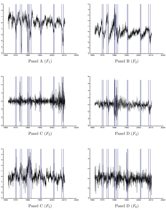
activity factor (as it loads on the output and labor market variables), the second factor is the bond yield factor, while the third factor is the price index factor. Moreover, the fourth factor represents an interest rate factor, the fifth factor loads on interest-rate spreads and inventories, while the sixth factor is a housing and output factor. Thus, to some extent the different factors capture information from different groups of macro variables. The time-series for each of the macro factors are plotted in Figure 2, which includes the NBER recession bars. We observe that the first, second, and fourth factors tend to decrease in recessions, while the third and fifth factors generally show a rise in volatility around the recession periods.

2.3

Financial state variables

The asset return data used in our empirical analysis correspond to the log value-weighted stock market return (rm), available from the Center for Research in Security Prices (CRSP). To construct the excess log stock return (r_me) we subtract the log one-month Treasury bill rate (rf), available from Kenneth French’s webpage. Both the log dividend-to-price ratio (d−p) and the log dividend growth (∆d) are based on a 12-month rolling sum of dividends. The dividend and price level data are associated with the Standard and Poors (S&P) 500 index and are obtained from Robert Shiller’s webpage.

Table2(Panel A) presents descriptive statistics for the financial variables used in the VAR analysis conducted in the following sections. The log dividend yield is quite persistent as indicated by the respective first-order autoregressive coefficient close to one. In comparison, the monthly log dividend growth, although less persistent, still shows a high persistence as indicated by the autocorrelation coefficient around 0.90. The high persistence of these two variables should be partially related with the way dividends are measured (12-month rolling sum).

macro factors estimated above. We can see that the stock market return is not significantly correlated with any of the factors, with all correlations below 0.20 in absolute terms, except with the fourth factor (0.20). The log dividend yield is also not significantly correlated with the macro factors, with the highest correlation occurring with the fifth factor (0.26). On the other hand, log dividend growth is positively correlated with the first and second factors (0.24 and 0.35 respectively).

3

Aggregate stock returns and macro variables

In this section we analyze whether the macro factors derived in the previous section drive the variation in the aggregate stock return, that is, whether they have an impact in the estimation of the components of the market return. In the next section, we analyse the case of the excess market return.

3.1

Methodology

Following Campbell (1991), the (unexpected) current log stock return can be decomposed into revisions of future expected log returns (discount-rate news) and revisions in expecta-tions of future log dividend growth (cash-flow news):

rm,t+1−Et(rm,t+1) = (Et+1−Et)

∞ X j=0 ρj∆dt+1+j −(Et+1−Et) ∞ X j=1 ρjrm,t+1+j ≡NCF,t+1−NDR,t+1, (4)

where Et denotes the conditional expectation at time t; NCF,t+1 represents cash-flow news;

and NDR,t+1 denotes discount-rate news. Equation (4) represents a dynamic present-value

relation that arises from the definition of stock return and by imposing a no-bubble condition at very long-horizons. The parameter ρ is a discount coefficient linked to the average log dividend-to-price ratio of the market portfolio. Following previous work (e.g.,Campbell and

Vuolteenaho (2004) and Maio (2013a, 2013c)), we calibrate ρ at 0.95121, which corresponds

to an annualized dividend yield of approximately 5%.

Given the dynamic identity in (4), we can produce the usual variance decomposition (in percentage) for the unexpected stock market return:

1 = Var (NCF,t+1) Var [rm,t+1−Et(rm,t+1)] + Var (NDR,t+1) Var [rm,t+1−Et(rm,t+1)] −2 Cov (NCF,t+1, NDR,t+1) Var [rm,t+1−Et(rm,t+1)] , (5)

where the first term on the right hand side represents the share of cash-flow news in driving the variation in the current market return, and the other two terms have a similar interpre-tation. Notice that due to the presence of the covariance term, −2 Cov (NCF,t+1, NDR,t+1),

the weight associated with each component of returns (NCF or NDR) can be greater than one to the extent that these variables are not orthogonal.

Following Campbell (1991), Campbell and Ammer (1993), and many others, we employ a first-order VAR to estimate the unobserved components of the market return, NCF and

NDR. The VAR equation below is assumed to govern the behavior of a state vector xt, which includes the log market return and other variables known in time t that help to forecast rm,t+1:

xt+1 =Axt+t+1, (6)

where A is the VAR coefficient matrix, and t+1 is a vector of zero-mean shocks.3

The components of the market return are estimated as follows:

NDR,t+1 =e10ρA(I−ρA) −1 t+1 =ϕ0t+1, (7) NCF,t+1 =rm,t+1−Et(rm,t+1) +NDR,t+1 =e10+e10ρA(I−ρA)−1t+1 = (e1+ϕ) 0 t+1, (8)

where e1 is an indicator vector that takes a value of one in the cell corresponding to the 3_{The VAR variables x}

t are previously demeaned, thus we do not include a vector of intercepts in the

position of the market return in the VAR;Iis an identity matrix; andϕ0 ≡e10ρA(I−ρA)−1 is the function that translates the VAR shocks into discount-rate news. In Equation (8), cash-flow news is the residual component of unexpected stock market returns, which has the advantage that one does not have to model directly the dynamics of aggregate dividends. This has been the standard identification method conducted in the related literature.

However, there has been some criticism about this identification strategy. Specifically, Chen and Zhao (2009) argue that any misspecification in the predictability of the market return, which directly affects the estimate of the discount-rate news series, will translate in-directly into cash-flow news since this is the residual component of the present-value relation (4). Moreover, by treating cash-flow news as the residual its weight might be overstated. Thus, directly identifying cash-flow news may lead to different estimates for cash-flow and discount-rate news, and hence a different variance decomposition for the market return. In contrast, both Campbell, Polk, and Vuolteenaho (2010) and Engsted, Pedersen, and Tang-gaard (2012)argue that with a properly specified VAR the two identification approaches are equivalent, and hence should yield relatively similar results.

To check the robustness of our results to the way cash-flow and discount-rate news are measured, and following Maio (2013a), we conduct an alternative identification procedure in which cash-flow news is now estimated directly, and discount-rate news is identified as the residual component of the (unexpected) market return:

NCF,t+1 =e20(I−ρA) −1 t+1 =λ0t+1 (9) NDR,t+1 =NCF,t+1−[rm,t+1−Et(rm,t+1)] =e20(I−ρA)−1−e10t+1 = (λ−e1) 0 t+1, (10)

where e2 is an indicator vector that takes a value of one in the cell corresponding to the position of log dividend growth in the VAR, and λ0 ≡ e20(I−ρA)−1 is the function that translates the VAR residuals into cash-flow news. Notice that both this identification and

the benchmark identification (7)-(8) are based on the Campbell (1991)dynamic identity for the market return.4

To assess the statistical significance of the weights associated with each component in the variance decomposition, we compute empirical t-statistics from a Bootstrap experiment. In this simulation, the VAR residuals are simulated 10,000 times and the first-order VAR, return components, and respective variance decomposition are estimated for each pseudo sample. The pseudo t-stats correspond to the individual shares (in the variance decomposi-tion) estimated for the original sample divided by the bootstrap standard errors. Details of the bootstrap experiment are presented in AppendixA.5

The state vector associated with the benchmark VAR for the market return (denoted by VAR I) is given by

xt≡[dt−pt,ft0,∆dt, rmt]

0

, (11)

where f0 ≡(F1t, ..., F6t) is the vector of six estimated macro factors. We use the same VAR specification under the two alternative identification schemes to preserve consistency and enable the comparison between both methods. The inclusion of the log aggregate dividend growth, ∆dt, is needed in order to identify cash-flow news under the alternative identification procedure. The inclusion of the log dividend-to-price ratio (d−p) is justified on the grounds that this variable is among the most important predictors of the market return in the pre-dictability literature.6 _{Specifically, based on the Campbell and Shiller (1988) present-value}

relation, the log dividend yield is theoretically justified as a valid predictor for both stock returns and dividend growth.7

4_{In related work,Garret and Priestley (2012)measure cash flow news based on a cointegration variable}

from annual dividends, price, and earnings. On the other hand, Da and Warachka (2009) and Da, Liu, and Schaumburg (2013)use direct measures of cash flow news based on revisions of equity analyst earnings forecasts.

5_{Similar statistical inference procedures are employed byVuolteenaho (2002),Campbell and Vuolteenaho}

(2004), andMaio (2013a).

6_{See Campbell and Shiller (1988), Fama and French (1988, 1989), Cochrane (1992), Hodrick (1992),}

Goetzmann and Jorion (1993), among many others.

7_{A recent branch of the return predictability literature analyses stock return and dividend growth}

pre-dictability from the dividend yield in association with theCampbell and Shiller (1988)present-value relation (see Cochrane (2008, 2011),Engsted and Pedersen (2010),Chen, Da, and Priestley (2012),Rangvid,

Schmel-The reduced or baseline VAR specification associated with VAR I excludes the macro factors:

xt≡[dt−pt,∆dt, rmt]

0

. (12)

The comparison between the baseline and benchmark specifications allows us to analyze the incremental effect associated with the macro factors in the variance decomposition for the market return, which represents the focus of our analysis.8

3.2

VAR estimates

The estimation results for VAR I are displayed in Table 3. To save space we only present the results for the return and dividend growth equations in the VAR, which represent the key regressions for the identification of discount-rate and cash-flow news. In the simple VAR specification that excludes the macro factors (columns 3 and 4), the dividend-to-price ratio forecasts positive market returns and the coefficient is significant at the 5% level according to Newey and West (1987) asymptotic t-statistics computed with one lag. We can also see that there is some degree of momentum in aggregate stock prices (returns) as indicated by the positive slope associated with the lagged market return, which is significant at the 10% level. The forecasting ratio is only 1%, which is in line with the explanatory power typically found in the literature for monthly predictive regressions of the market return.

In the equation for log dividend growth, the slope associated with lagged dividend growth (0.90) is strongly significant (1% level). On the other hand, none of the other two variables can forecast aggregate cash flows as indicated by the very lowt-stats. The forecasting ratio in the monthly dividend growth equation is as large as 80%, due to the large persistence of this variable. Therefore, these results show that at the monthly frequency (and using cumulative annual dividends in the computation of bothd−p and ∆d), it is much easier to

ing, and Schrimpf (2012),Maio and Santa-Clara (2013), among others).

8_{Chen and Zhao (2009) (Section 4.3) incorporate in the VAR five factors (estimated from principal}

component analysis) from a “large set of state variables that can predict stock returns”. They do not present, however, any information about the identity of these state variables.

forecast aggregate dividend growth than aggregate stock returns.

The results for the VAR benchmark specification that includes the six macro factors are presented in columns 1 and 2 of Table 3. In the regression for the market return, the coefficient (and respective t-stat) associated with d−p is similar to the corresponding estimate in the baseline VAR, which means that the macro factors are relatively orthogonal to this state variable, as shown in Table 2. In contrast, the positive slope for the lagged market return decreases in magnitude and is no longer significant at the 10% level. Among the six macro factors, only F2 (at the 1% level) and F4 (5% level) are significant forecasters

of the market return, conditional on the other state variables. The R2 estimate in the return equation is 4%, showing that the addition of the six factors (specifically, the two factors mentioned above) leads to a (modest) increase in the forecasting power of the market return at the one-month horizon. These results are somewhat consistent with the findings in Ludvigson and Ng (2007) showing that macro factors add relatively small forecasting power for the market return at the quarterly horizon, when controlling for other predictors like the consumption-to-wealth ratio (cay) or the relative T-bill rate.910

In the equation for dividend growth, the slopes (and respective t-stats) associated with both d−p and lagged ∆d are similar to the corresponding estimates in the baseline spec-ification. All the factors forecast significantly positive dividend growth, and this effect is statistically significant (5% or 1% level) in the cases of F1, F2, F5, and F6. However, the

forecasting ratio of 81% shows that the inclusion of the six macro factors has quite marginal impact for forecasting aggregate dividend growth. In other words, the information about fu-ture dividend growth contained in the macro factors is already incorporated in the dividend 9_{See Table 2 in their paper. Notice thatLudvigson and Ng (2007)use non-linear transformations of the}

original macro factors in their predictive regressions, which may lead to an increased forecasting power. In our case, to preserve the economic intuition associated with each factor, the VAR only contains the original factors.

10_{There is evidence of greater stock return predictability from macro variables at the quarterly or lower}

fre-quencies (seeLettau and Ludvigson (2001),Rangvid (2006), Cooper and Priestley (2009, 2013),Hsu (2009), among others). This increased forecasting power should be partially related with the higher persistence of macro variables at lower frequencies. Our empirical analysis is based on monthly data in order to achieve greater statistical power on the econometric tests, similarly toLudvigson and Ng (2009).

yield and especially in the lagged dividend growth.

3.3

Variance decomposition

The benchmark variance decomposition for the market return is presented in Table4, Panel A. In the baseline VAR specification (excluding the macro factors, row 2) we can see that the bulk of variation in the current market return is discount-rate news, which accounts for 68% of the variance of the realized return, around two times the share associated with cash-flow news (34%). The two components of the market return are nearly orthogonal (correlation of 0.02) so that the covariance term, −2 Cov(NCF,t+1, NDR,t+1), has a very marginal role,

representing only 2% of the total variance in absolute value. Still, the very low empirical

t-stats show that all components of the stock market return decomposition are estimated with substantial sampling error.

These results are in line with some of the previous evidence showing that the dominant component of the (unexpected) market return is discount rate news (e.g., Campbell (1991), Campbell and Ammer (1993), Campbell and Vuolteenaho (2004), Bernanke and Kuttner (2005), and Maio (2013a, 2013e), among others), despite the decrease in the magnitude of return predictability observed in recent years, which directly affects the discount-rate news series.11 _{There is also evidence showing an increase in the importance of cash-flow news in}

driving recent movements in stock prices (see Campbell, Giglio, and Polk (2013)).12

By adding the macro factors to the VAR estimation (row 1) the variance decomposition does not change in a significant way. The weights associated with NDR and NCF increase only marginally to 73% and 37% respectively, while the share for the covariance term is also 11_{Specifically,Maio (2013c)by using a different VAR specification shows that the decline in stock return}

predictability in recent years leads to a lower share of discount rate news in the market return decomposition. On the other hand,Chen and Zhao (2009)show that small changes in the choice of state variables included in the VAR lead to sharp differences in the variance decomposition for the market return. In related work, Sadka (2007)finds evidence of a similar weight for cash flow and discount rate news in the aggregate stock return decomposition.

12_{At the portfolio or stock levels there is more clear evidence that the dominant component of equity}

returns is cash flow news (seeVuolteenaho (2002),Callen and Segal (2004),Callen, Hope, and Segal (2005), andMaio (2013a), among others).

marginally larger in magnitude (-9%). The bootstrapped t-stats associated with discount rate and cash-flow news are now 1.52 and 1.81 respectively, while the covariance term is estimated with very low precision. Thus, this result suggests that excluding the information associated with a lot of macro variables does not change the relative importance of discount-rate and cash-flow news in driving the current aggregate stock return. However, by including the macro factors in the VAR, we obtain more precise estimates for the shares associated with bothNDR and NCF.

The results for the alternative identification of the market return components in the baseline specification (Panel B, row 2) show that the share for discount rate news is sig-nificantly higher than in the benchmark identification (113%). This comes as a result of a slightly lower share for cash flow news (24%), and especially, a larger absolute share for the covariance term, which represents now around -38% of the market variance (the correlation of the two components is now 0.36).13 _{However, all the shares are estimated with very low}

precision as indicated by the bootstrappedt-stats. When we include the six macro factors in the VAR, the variance decomposition for the stock return is basically the same, similarly to the benchmark identification case. The main difference refers to the highert-stats, especially the share associated with NDR, which is now 2.34 standard errors away from zero. Hence, incorporating the macro factors in the VAR leads to more precise estimates of the individual shares in the return decomposition, as in the benchmark identification case.

3.4

Lagged factors

We conduct the variance decomposition by using the lagged realizations of the six macro factors in the VAR. The reason is that some of the original macro variables (e.g., industrial production or CPI) become publicly available with a lag (usually one month). Thus, an investor might not have had access to this information when forecasting stock returns in real 13_{This result showing that the two alternative identification methods yield different results might be related}

with the fact that log dividends (annualized) are not measured on the same time interval as log prices and log returns, and thus theCampbell (1991)decomposition is not strictly satisfied in this case.

time. On the other hand, other variables like short-term interest rates or bond yields are available in real time. Untabulated results show that the variance decomposition based on the lagged macro factors (in both identification schemes) is very close to the one based on the raw macro factors.

3.5

Innovation in factors

We redo the variance decomposition by including in the VAR the innovations in the macro factors rather than the original time-series obtained from Section 2. The idea is to use the “surprise” or unexpected component of the macro variables in order to forecast stock returns or dividend growth. The innovation in each factor is obtained by fitting an AR(1) process for each variable,

Fj,t+1 =φ0+φ1Fj,t+uj,t+1, j = 1, ...,6, (13)

and then using the innovations, f∗0 ≡ (u1t, ..., u6t), in the VAR employed to estimate the components of the stock return,

xt≡[dt−pt,ft∗0,∆dt, rmt]

0

. (14)

Untabulated results show that the variance decomposition obtained from using the in-novations in the macro factors is quite similar to the variance decomposition based on the original factors, and this holds for both identification schemes. Thus, using the surprise elements of the macro factors does not change in a significant way the predictive power for stock returns and dividend growth.

3.6

Alternative macro variables

We estimate the first-order VAR by using individual macro variables which are “represen-tative” of each of the common macro factors. The representative variable for each common factor corresponds to the original macro variable that yields the highestR2 in regression (3)

above. The motivation for this exercise is two-fold. First, the common macro factors are estimated with error, which can have an impact on the estimated VAR slopes, and thereby on the variance decomposition for the market return. Second, using raw macro variables ac-counts for the “look-ahead” bias associated with the estimated common factors (since their estimation is based on the full sample), which can impact the slopes estimates within the VAR.

The macro variables used in the VAR, and associated with factors 1 to 6, are “Employees on nonfarm payrolls–goods-producing” (series number 29); “Spread between Moodys Baa corporate bond yield and Federal funds effective rate” (98); “CPI-U: commodities” (115); “1-year Treasury bond yield” (86); “Spread between Treasury-bill 6-month rate and Federal funds effective rate” (93); and “Housing starts” (48), respectively. A detailed description of the variables is provided in Table A.1. Results not tabulated show that the variance de-composition obtained from using the raw macro variables, in place of the common factors, is basically the same as the variance decomposition from the original factors, and this holds for both identification schemes. Thus, any potential “look-ahead” bias from using the estimated common factors is not driving our results.

3.7

Alternative measure of dividends

Following most of the return predictability literature, our measure of dividends is based on the cumulative dividend over the previous 12 months to account for dividend seasonality (see Ang and Bekaert (2007),Goyal and Welch (2008),Chen (2009), among many others). In this section we compute the log dividend-to-price ratio and log dividend growth based on monthly dividends. According to theCampbell and Shiller (1988)andCampbell (1991)present-value relations, the return, dividend yield, and dividend growth should be based on log dividends and log prices measured over the same time interval (monthly in our case). Thus, by using annualized dividends in the construction of d−p and ∆d, the Campbell and Shiller (1988) present-value relation—and the resulting predictability patterns fromd−p—are not satisfied.

Following Cochrane (2008), we construct the aggregate monthly dividend-to-price ratio and dividend growth by combining the monthly series on the total return and return without dividends associated with the value-weighted CRSP index.

Untabulated results show that in the baseline VAR specification (excluding the macro factors) the bulk of variation in the current market return is cash-flow news, which accounts for more than 100% (about 122%) of the variance of the realized return, while the share associated with discount-rate news is only 4%. The two components of the market return are positively correlated (0.59) so that the covariance term,−2 Cov(NCF,t+1, NDR,t+1), represents

about 26% of the total variance in absolute value. The very small weight associated with discount-rate news is a consequence of the new measure of d−p, which is significantly less persistent than the conventional proxy, and thus has much less forecasting power for the stock market return. More relevant to the focus in this paper, by adding the macro factors to the VAR estimation, the variance decomposition changes only slightly. The weights associated with NDR and NCF increase only marginally to 17% and 125% respectively, while the share for the covariance term shows a larger increase in magnitude (to -42%).14

The variance decompositions based on the alternative VAR identification are quite close to those based on the direct estimation of discount-rate news in both the baseline and augmented VAR specifications. This is a consequence of the large forecasting power of

d−p for dividend growth under the new proxy for dividends. Thus, with the new dividend measure the order of identification of the return components (estimating discount-rate news directly, or in alternative, deriving it as the residual component) does not make a difference to the relative share of discount-rate and cash-flow news in the stock return variance. Hence, our results are consistent with the claims fromCampbell, Polk, and Vuolteenaho (2010) and Engsted, Pedersen, and Tanggaard (2012).

14_{Given theCampbell and Shiller (1988)present-value relation for the log dividend-to-price ratio, one could}

be tempted to conclude that d−p is the only relevant state variable for the stock return decomposition. However, this present-value relation only holds at very long horizons, and in fact the evidence of predictability of future returns and dividend growth fromd−pat short horizons (as in the case of the first-order VAR being estimated here) is relatively weak (seeCochrane (2008)andMaio and Santa-Clara (2013), among others).

3.8

Alternative VAR specification

We estimate an alternative VAR specification that excludes dividend growth,

xt ≡[dt−pt,ft0, rmt]

0

. (15)

This specification is in line with most of the related literature, which typically does not include dividend growth in the set of VAR state variables. Moreover, this specification might allow for a cleaner estimation of the effect of the macro factors in the return decomposition given the positive correlations between dividend growth and some of these variables, as documented in Table 2. In untabulated results, the shares associated with discount rate news and cash flow news are 83% and 21% respectively, while the covariance term plays a negligible role. When we exclude the macro factors from the VAR the variance decomposition is basically the same.

3.9

Sensitivity to

ρ

We analyze the sensitivity of the results to the value of the log-linearization parameter, ρ. We calibrate two alternative values for the discount factor, 0.93121 and 0.97

1

12. Untabulated

results show that the benchmark return decomposition is quite sensitive to this parameter, with higher values of ρ corresponding to larger shares of discount rate news on the total return variance. However, for the purposes of this paper, by adding macro factors to the VAR state vector the variance decomposition does not change in a meaningful way.

Overall, the punch line from the results presented in this section is quite simple: inclusion of the macro factors in addition to d−p (as well as lagged dividend growth and lagged market return) does not add significant information to the estimation of the components of the aggregate stock return.

4

Macro variables and the excess market return

In this section, we analyze the impact of the macro variables on the components of the excess stock market return. In fact, most of the related literature focuses on the determinants of the components of excess returns rather than stock returns.

4.1

Methodology

Following Campbell (1991) and Campbell and Ammer (1993), we can derive a dynamic present-value relation for the unexpected excess stock return:

re_m,t+1−Et(r_m,te ₊₁) = (Et+1−Et)

∞ X j=0 ρj∆dt+1+j −(Et+1−Et) ∞ X j=1 ρjre_m,t+1+j −(Et+1−Et) ∞ X j=1 ρjrf,t+1+j ≡NCF,t+1−NDR,t+1−NF,t+1, (16) wherere

m,t+1 ≡rm,t+1−rf,t+1denotes the excess log return andNF,t+1 ≡(Et+1−Et)

P∞

j=1ρ

j_r f,t+1+j represents the revision in future short-term interest rates (interest-rate news). The main dif-ference relative to the dynamic identity for stock returns in Equation (4) is the inclusion of

NF,t+1 due to the fact that we are now working with excess log returns rather than log

re-turns. Thus, according to this present-value relation, a positive shock in excess stock returns today must be matched by positive shocks in future dividend growth rates, and/or negative shocks in both future excess returns and short-term interest rates. A full derivation of the decomposition in (16) is presented in AppendixB.

Given the present-value relation in (16), the variance decomposition for the excess stock return is given by 1 = Var (NCF,t+1) Varre m,t+1−Et(rm,te +1) + Var (NDR,t+1) Varre m,t+1−Et(rem,t+1) + Var (NF,t+1) Varre m,t+1−Et(rem,t+1) −2 Cov (NCF,t+1, NDR,t+1) Varre m,t+1−Et(rem,t+1) + 2 Cov (NDR,t+1, NF,t+1) Varre m,t+1−Et(rm,te +1) − 2 Cov (NCF,t+1, NF,t+1) Varre m,t+1−Et(rem,t+1) . (17)

The additional terms relative to the variance decomposition for the stock return in the previous section arise from the presence of interest-rate news.

In the benchmark identification of the excess stock returns’ components, interest rate news, equity-premia news, and cash-flow news are estimated in a similar way to Campbell (1991), Campbell and Ammer (1993), and Hollifield, Koop, and Li (2003):

NF,t+1 =e30ρA(I−ρA) −1 t+1 =ψ0t+1, (18) NDR,t+1 =e10ρA(I−ρA)−1t+1 =ϕ0t+1, (19) NCF,t+1 = (Et+1−Et)rm,te +1+NDR,t+1+NF,t+1 = (e1+ϕ+ψ)0t+1, (20)

where e1 is the indicator vector that assigns a value of one in the cell corresponding to the position of the excess stock market return in the VAR, and ϕ0 ≡ e10ρA(I −ρA)−1

is the function that relates the VAR shocks with revisions in expected future excess stock returns. Similarly, e3 identifies the position of the log interest rate within the VAR, and ψ0 ≡e30ρA(I−ρA)−1 is the function that relates the VAR shocks with interest-rate news.

As in the last section, the alternative identification of the excess stock returns’ compo-nents directly estimates cash-flow news, and implies discount-rate news as the residual of the present-value relation:

NCF,t+1 =e20(I−ρA)

−1

t+1 =λ0t+1, (21)

NDR,t+1 =NCF,t+1−[rm,t+1−Et(rm,t+1)]−NF,t+1

= (λ−e1−ψ)0t+1. (22)

The state vector associated with the VAR for excess returns is given by

xt≡[rf t, dt−pt,ft0,∆dt, remt]

0

where the only differences relative to the benchmark VAR in the last section is the inclusion of the log short-term interest rate,rf t—which is necessary to identify interest rate news—and the fact that we now have the excess stock return instead of the nominal equity return.

As in the previous section, the associated baseline VAR excludes the macro factors:

xt≡[rf t, dt−pt,∆dt, remt]

0

. (24)

4.2

VAR estimates

The estimation results for the VAR associated with the aggregate equity premium are pre-sented in Table 5. To save space we only present the estimates for the excess stock return, dividend growth, and log interest rate equations, which represent the key equations for the identification of the unobserved components of the excess stock return. In the case of the baseline specification without macro factors (columns 4 to 6), the forecasting ratio in both the dividend growth and equity premium equations is the same as in the benchmark VAR estimated in the last section, thus suggesting that rf does not add forecasting power for both excess stock returns and dividend growth.15 _{The slope for the dividend yield in the}

excess return equation is now only marginally significant (10% level) suggesting that the log dividend-to-price ratio has greater forecasting ability for the aggregate stock return than the equity premium. The log interest rate is relatively persistent as indicated by the autoregres-sive coefficient of 0.94, which is strongly significant (1% level). Moreover, both d−p and ∆dforecasts a increase in the monthly T-bill rate, and these slopes are significant at the 1% level. The fit of the interest rate equation is fairly large (92%), which is partially explained by its high persistence.

When we include the six macro factors (columns 1 to 3), the forecasting ratios in the interest rate and dividend growth regressions increase only marginally, thus showing that 15_{There is evidence showing that the change or innovation in short-term interest rates is a significant}

forecaster of excess stock returns, at least for short-horizons (seeCampbell (1991),Hodrick (1992),Campbell and Ammer (1993), Maio (2013b, 2013e), among others).

the macro factors as a whole do not add relevant forecasting power. In the regression for

rf,t+1, it follows thatF1,F2,F5, andF6 significantly forecast an increase in the future

short-rate, while F4 significantly predicts a decline. The autoregressive coefficient (0.92) is only

marginally lower than in the baseline VAR, while the lagged equity premium forecasts an increase in future interest rates, and this effect is marginally significant (10% level). On the other hand, dividend growth is no longer a significant predictor of the T-bill rate. In the dividend growth equation, F1, F2, and F6 forecast an increase in future dividend growth,

and the respective slopes are statistically significant (marginally so in the case of the second factor). In the equation for the equity premium, the forecasting ratio increases to 4% (from 1% in the restricted VAR) indicating that the macro factors jointly have some incremental forecasting ability for excess stock returns, similarly to the VAR for the market return in the last section. However, individually only the second and fourth factors are significant predictors of the equity premium, as in the case of the stock return.

4.3

Variance decomposition

The variance decomposition for the excess stock market return is presented in Table6. In the restricted VAR (Panel A, row 2), both cash flow and discount rate news play a similar role in driving excess stock returns with shares of 34% and 35% respectively. Interest-rate news play a smaller role in moving the excess market return as illustrated by the weight of 18% over the return variance. The covariance terms associated with cash flow news also play a marginal role, with shares around 10% in absolute terms as a result of the small correlations among the respective equity premium components. On the other hand, the share associated with 2 Cov(NDR, NF) represents 15% of the excess return variance. However, only the weights associated with the variances of discount rate and cash flow news are at least one standard error away from zero.

When we include the macro factors in the VAR estimation (row 1), the weights for each term in the variance decomposition do not change significantly. The weights associated with

NDR and NCF increase marginally to 40% and 37% respectively, while the share of interest rate news declines to 14%. The weights associated with discount rate and cash flow news are now 1.54 and 2.02 standard errors away from zero, while the other shares remain highly insignificant. Thus, as in the last section, by incorporating the macro variables in the VAR estimation we obtain more precise estimates in the variance decomposition of the excess stock return.

The results for the alternative identification of the excess stock return components (Panel B) show that all the weights are relatively similar under both the restricted and augmented VAR (that includes the macro variables). In the full VAR, discount rate news accounts for 69% of the variation in the excess stock return, and this estimate is highly significant (3.14 standard errors away from zero). The shares associated with cash flow and interest rate news have significantly lower magnitudes than discount rate news (27% and 14%, respectively), and both estimates have significantly higher sampling error. When we exclude the macro factors, the shares associated with the variances of NDR, NCF, and NF are 63%, 26%, and 18% respectively, but only the share for discount rate news is at least one standard error greater than zero.

Overall, the results of this section largely confirm the findings in the previous section: The macro factors play a relatively marginal role for the variance decomposition of the excess stock return. Thus, the relative importance of the components of excess stock returns (cash-flow, discount-rate, and interest-rate news) does not change significantly by including the macro factors in a VAR that already contains the aggregate dividend yield or the T-bill rate. Therefore, such results suggest that these financial state variables already incorporate most of the relevant information required to identify the components of the equity premium.

5

Implications for the cross-section of stock returns

5.1

Methodology

Following theCampbell (1993)version of theMerton (1973)ICAPM, Campbell and Vuolteenaho derive the following two-factor model:

E(ri,t+1−rf,t+1) +

σ2

i

2 =γωCov(ri,t+1, NCF,t+1)−ωCov(ri,t+1, NDR,t+1), (25)

where ri,t+1 denotes the log return for asset i; σi2 ≡ Var(ri,t+1) is the respective variance;

rf,t+1 is the log risk-free rate; and γ denotes the coefficient of relative risk aversion. This

version of the Campbell and Vuolteenaho ICAPM is based on the first-order condition of the consumption-portfolio choice problem for an investor with a reference portfolio invested on the stock index and a risk-free asset:

rp,t+1 ≈ωrm,t+1+ (1−ω)rf,t+1, (26)

where rp,t+1 denotes the log portfolio return andrm,t+1 is the log return on the stock index.

The advantage of this specification is that the risk price for the discount-rate covariance (beta) is freely estimated in the cross-section of stock returns rather than being fixed at -1, as in the benchmark specification used in Campbell and Vuolteenaho (2004):

E(ri,t+1−rf,t+1) +

σ2

i

As inCampbell and Vuolteenaho (2004), in the pricing equation taken to the data we replace excess log returns by excess simple returns on the left hand side of the equation:

E(Ri,t+1−Rf,t+1) = bCF Cov(ri,t+1, NCF,t+1) +bDRCov(ri,t+1, NDR,t+1), (28)

where bCF ≡ γω denotes the risk price for cash-flow news, and bDR ≡ −ω is the discount-rate risk price. Thus, according to this pricing equation, the signs of bCF and bDR should be positive and negative, respectively.

Although the pricing equation above contains no intercept, as a robustness check, we also test an alternative version of the model that includes an intercept:

E(Ri,t+1−Rf,t+1) =b0 +bCFCov(ri,t+1, NCF,t+1) +bDRCov(ri,t+1, NDR,t+1). (29)

If the two-factor model is specified correctly, the intercept should be indistinguishable from zero.

To estimate the model above we employ first stage GMM (Hansen (1982), Cochrane (2005)), which uses as weighting matrix the identity matrix. This procedure is equivalent to an OLS cross-sectional regression of average excess returns on factor covariances (betas), and enables us to assess whether the model can explain the returns of a set of equity portfolios. The firstN sample moments correspond to the pricing errors for each of theN test assets:

gT(b)≡ 1 T T X t=0           

(Ri,t+1−Rf,t+1)−bCFri,t+1(NCF,t+1−µCF)−bDRri,t+1(NDR,t+1−µDR)

NCF,t+1−µCF

NDR,t+1−µDR

=0,

i= 1, ..., N, (30)

in (30) enable us to estimate the factor means; thus, the standard errors of the estimated covariance risk prices (obtained from the firstN moments) account for the estimation error in the factor means, as in Cochrane (2005) (Chapter 13), Maio and Santa-Clara (2012), and Maio (2013c). The asymptotic t-statistics for the risk price estimates are based on heteroskedasticity-robust standard errors (White (1980)); that is, no lags of the moment functions are considered in the computation of the spectral density matrix, as in Cochrane (2005) and Maio (2013c, 2013d).

The test assets are the 25 portfolios sorted according to size and book-to-market (SBM25), which represent the focus of the empirical asset pricing literature. SBM25 are obtained from Kenneth French’s website. To compute excess portfolio returns we subtract the one-month T-bill rate from the raw returns. The sample used in the asset pricing tests is 1964:02 to 2010:09. The estimates for cash-flow and discount-rate news are those from the VAR associated with the excess market return, estimated in the previous section.

A test for the null hypothesis that the N pricing errors are jointly equal to zero (that is, the model is perfectly specified) is given by

ˆ

α0Var ( ˆd α)

†

ˆ

α∼χ2(N −K), (31)

where K denotes the number of factors (K = 2 in the ICAPM with no intercept); ˆα is the (N ×1) vector of cross-sectional pricing errors; and Var ( ˆd α)

†

denotes a pseudo-inverse for the covariance matrix of the pricing errors, dVar ( ˆα).

A more robust and intuitive goodness-of-fit measure to evaluate the overall pricing ability of the two-factor model is the cross-sectional OLS coefficient of determination,

R2 = 1− PN i=1αˆ 2 i PN i=1R 2 i , (32) whereRi = _T1 PT−1 t=0 (Ri,t+1−Rf,t+1)−_N1 PN i=1 n 1 T PT−1 t=0 (Ri,t+1−Rf,t+1) o

denotes the (cross-sectionally) demeaned (average) excess returns; ˆαi represents the pricing error for asset i;

and ˆαi stands for the (cross-sectionally) demeaned pricing errors. R2 measures the fraction of the cross-sectional variance in average excess returns explained by the model.

5.2

Empirical results

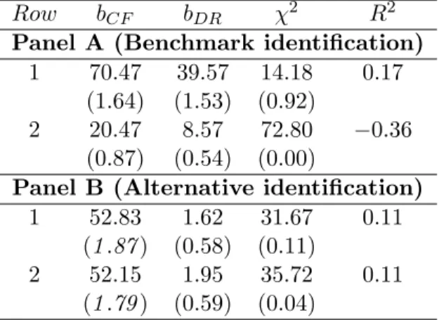
The results for the cross-sectional test of the benchmark specification of the ICAPM (without intercept) are presented in Table 7. When we consider the ICAPM based on the restricted VAR (row 2 in each panel), only under the alternative identification (of cash flow and discount rate news, Panel B) do we have a positive explanatory ratio, but the level is quite modest (11%). When the ICAPM is based on the benchmark identification of the equity premium components we have a negative R2 estimate (-36%), that is, the ICAPM performs worse than a model that predicts constant expected excess returns in the cross-section of equities. When we include the macro factors in the VAR estimation (row 1) the results for the ICAPM are mixed. If we use the alternative identification of cash flow and discount rate news the fit of the model does not change as the cross-sectional R2 _{stays at 11%. On}

the other hand, the two-factor model based on the benchmark identification of the equity premium components shows an increased explanatory power for the cross-section of stock returns, in comparison to the model based on the restricted VAR. However, the fit is still very modest as indicated by the R2 estimate of 17%. Despite the low explanatory power, the two-factor model (based on the macro variables) is not rejected by the specification test, with p-values clearly above 5%. This shows how misleading the χ2_{-test can be in some}

cases, that is, the null (that the pricing errors are equal to zero) is not rejected because the inverse of the variance matrix is underestimated, rather than as a result of low pricing errors. Moreover, the discount-rate risk prices are in all cases estimated positively (although not statistically significant), which is inconsistent with the theory underlying the two-factor ICAPM as discussed above.

The relatively poor performance of the two-factor ICAPM is consistent with the evidence inMaio (2013d)(for a shorter sample) showing that the fit of the model from Campbell and

Vuolteenaho (2004)relies critically not only on the inclusion of the value spread in the VAR used to estimate the factors (cash flow and discount rate news), but also on the computation of Dimson (1979) betas, which include the covariances with the lagged factors.

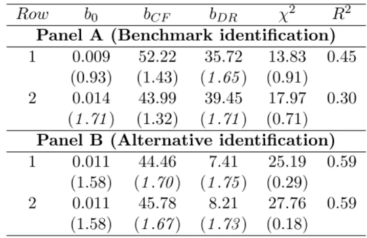
In Table8, we present the estimation results when an intercept is included in the ICAPM pricing equation. For the ICAPM based on the restricted VAR we see that the estimates for the excess zero beta rate are economically significant (above 1% per month), and these estimates are statistically significant in the version based on the benchmark identification. This suggests that the two-factor model is misspecified, that is, there are relevant missing risk factors in the model. The explanatory ratios are now positive, especially in the ICAPM version based on the alternative identification of cash flow and discount rate news (59%). However, this higher fit is basically due to the inclusion of the intercept in the pricing equation, which represents model’s misspecification.

When the ICAPM is based on the benchmark VAR that contains the macro factors, under the benchmark identification the estimate for the intercept decreases in magnitude relative to the version based on the restricted VAR, and is no longer statistically significant. Yet, in the version based on the alternative identification, the estimate for the intercept is the same as in the model based on the restricted VAR. The fit of the model increases slightly relative to the version based on the VAR without the macro factors when we use the benchmark identification method. However, similarly to the ICAPM specification without intercept, when we use the alternative identification the fit of the model does not change by including the macro variables in the VAR. For both versions of the ICAPM (restricted and benchmark VAR), the risk price estimates for the discount-rate factor have the wrong sign (positive) in all cases, and all of these estimates are now statistically significant at the 10% level.

The results of this section can be summarized as follows: using macro factors to iden-tify the components of the excess stock market return does not significantly improve the explanatory power of the Campbell and Vuolteenaho (2004)two-factor model in pricing the

size-BM portfolios. Actually, in some cases the fit of the model does not change at all by incorporating the information associated with the macro factors. An implication of these results is that macro variables (unrelated to stock prices) do not seem to be valid ICAPM state variables in terms of explaining risk premia in the cross-section of stocks.

6

Conclusion

We conduct a variance decomposition for stock returns by incorporating the information associated with a large macroeconomic panel data set. This analysis enables us to check whether macro variables convey relevant information to forecast stock returns in addition to the variables usually employed in the predictability and return decomposition literatures— aggregate financial ratios (such as the dividend yield or earnings yield), bond yield spreads (such as the slope of the yield curve or the credit risk spread), or short-term interest rates.

Using dynamic factor analysis, we estimate six common macroeconomic factors that sum-marize information from a panel of 124 macro variables, which can be broadly classified into different categories: output and income; employment and labor force; housing; manufactur-ing, inventories and sales; money and credit; interest rates and bond yields; foreign exchange; and price indices. We then estimate a first-order VAR containing the six macro factors, the aggregate stock return, the aggregate dividend growth, and the market dividend yield (d−p). This VAR specification is used to identify the components of the market return—discount-rate and cash-flow news. We compare the variance decomposition for stock returns with a restricted VAR that excludes the macro factors; that is, it does not incorporate the informa-tion from the large macro panel set. The results show that the inclusion of the macro factors in addition to d−p does not add significant information in estimating the components of aggregate stock returns.

We also analyze the impact of the macro variables on the components of the equity premium by using a VAR specification that includes the excess stock market return and the

T-bill rate. Overall, the results show that the macro factors play a relatively marginal role for the variance decompositions of the excess stock return. Thus, the relative importance of the components of excess stock returns (cash-flow, discount-rate, and interest-rate news) does not change significantly by including the macro factors in a VAR that already contains the aggregate dividend yield and the short-term interest rate. In other words, the macro variables do not add enough forecasting power (enough to change the relative importance of the excess return components) to a VAR that already contains the financial variables in terms of predicting the equity premium or dividend growth.

We use the time-series of cash-flow and discount-rate news to test the two-factor In-tertemporal CAPM (ICAPM) from Campbell and Vuolteenaho (2004). The results indicate that using macro factors to identify the components of the excess stock market return does not improve significantly the explanatory power of the two-factor model in pricing the 25 size/book-to-market portfolios.

References

Ang, A., and G. Bekaert, 2007, Stock return predictability: Is it there? Review of Financial Studies 20, 651–708.

Baele, L., G. Bekaert, and K. Inghelbrecht, 2010, The determinants of stock and bond return comovements, Review of Financial Studies 23, 2374–2428.

Bai, J., 2010, Equity premium predictions with adaptive macro indices, Working paper, Federal Reserve Bank of New York.

Bai, J., and S. Ng, 2002, Determining the number of factors in approximate factor models, Econometrica 70, 191–221.

Barnett, W., and M. Chauvet, 2011, How better monetary statistics could have signaled the financial crisis, Journal of Econometrics 161, 6–23.

Bernanke, B., and K. Kuttner, 2005, What explains the stock market’s reaction to Federal Reserve policy? Journal of Finance 60, 1221–1257.

Bianchi, F., 2011, Rare events, agents’ expectations, and the cross-section of asset returns, Working paper, Duke University.

Botshekan, M., R. Kraeussl, and A. Lucas, 2012, Cash flow and discount rate risk in up and down markets: What is actually priced? Journal of Financial and Quantitative Analysis 47, 1279–1301.

Boyd, J., J. Hu, and R. Jagannathan, 2005, The stock market’s reaction to unemployment news: Why bad news is usually good for stocks, Journal of Finance 60, 649–672.

Callen, J., O. K. Hope, and D. Segal, 2005, Domestic and foreign earnings, stock return variability, and the impact of investor sophistication, Journal of Accounting Research 43, 377–412.

Callen, J., and D. Segal, 2004, Do accruals drive firm-level stock returns? A variance de-composition analysis, Journal of Accounting Research 42, 527–560.

Campbell, J., 1991, A variance decomposition for stock returns, Economic Journal 101, 157–179.

Campbell, J., 1993, Intertemporal asset pricing without consumption data, American Eco-nomic Review 83, 487–512.

Campbell, J., 1996, Understanding risk and return, Journal of Political Economy 104, 298– 345.

Campbell, J., and J. Ammer, 1993, What moves the stock and bond markets? A variance decomposition for long-term asset returns, Journal of Finance 48, 3–26.

Campbell, J., S. Giglio, and C. Polk, 2013, Hard times, Review of Asset Pricing Studies 3, 95–132.

Campbell, J., S. Giglio, C. Polk, and R. Turley, 2012, An intertemporal CAPM with stochas-tic volatility, Working paper, Harvard University.

Campbell, J., C. Polk, and T. Vuolteenaho, 2010, Growth or glamour? Fundamentals and systematic risk in stock returns, Review of Financial Studies 23, 305–344.

Campbell, J., and R. Shiller, 1988, The dividend price ratio and expectations of future dividends and discount factors, Review of Financial Studies 1, 195–228.

Campbell, J., and T. Vuolteenaho, 2004, Bad beta, good beta, American Economic Review 94, 1249–1275.

Chen, J., 2003, Intertemporal CAPM and the cross-section of stock returns, Working paper, University of California, Davis.

Chen, L., 2009, On the reversal of return and dividend growth predictability: A tale of two periods, Journal of Financial Economics 92, 128–151.

Chen, L., Z. Da, and R. Priestley, 2012, Dividend smoothing and predictability, Management Science 58, 1834–1853.

Chen, L., and X. Zhao, 2009, Return decomposition, Review of Financial Studies 22, 5213– 5249.

Cochrane, J., 1992, Explaining the variance of price-dividend ratios, Review of Financial Studies 5, 243–280.

Cochrane, J., 2005, Asset pricing, Princeton University Press, Princeton, NJ.

Cochrane, J., 2008, The dog that did not bark: A defense of return predictability, Review of Financial Studies 21, 1533–1575.

Cochrane, J., 2011, Presidential address: Discount rates, Journal of Finance 66, 1047–1108. Connor, G., and R. Korajczyk, 1986, Performance measurement