Bayesian cylindrical data modeling
using Abe-Ley mixtures
N. Sadeghianpourhamamia,∗, D. F. Benoitb, D. Deschrijvera, C. Develdera
aGhent University – imec, IDLab, Dept. of Information Technology, Technologiepark Zwijnaarde 15, 9052 Ghent, Belgium bGhent University, Faculty of Economics and Business Administration,
Tweekerkenstraat 2, 9000 Ghent, Belgium
Abstract
This paper proposes a Metropolis-Hastings algorithm based on Markov chain
Monte Carlo sampling, to estimate the parameters of the Abe-Ley distribution,
which is a recently proposed Weibull-Sine-Skewed-von Mises mixture model, for
bivariate circular-linear data. Current literature estimates the parameters of
these mixture models using the expectation-maximization method, but we will
show that this exhibits a few shortcomings for the considered mixture model.
First, standard expectation-maximization does not guarantee convergence to a global optimum, because the likelihood is multi-modal, which results from the
high dimensionality of the mixture’s likelihood. Second, given that
expectation-maximization provides point estimates of the parameters only, the uncertainties
of the estimates (e.g., confidence intervals) are not directly available in these
methods. Hence, extra calculations are needed to quantify such uncertainty. We
propose a Metropolis-Hastings based algorithm that avoids both shortcomings
of expectation-maximization. Indeed, Metropolis-Hastings provides an
approx-imation to the complete (posterior) distribution, given that it samples from the
joint posterior of the mixture parameters. This facilitates direct inference (e.g.,
about uncertainty, multi-modality) from the estimation. In developing the
algo-∗Corresponding author
Email addresses: [email protected](N. Sadeghianpourhamami), [email protected](D. F. Benoit),[email protected](D. Deschrijver), [email protected](C. Develder)
rithm, we tackle various challenges including convergence speed, label switching
and selecting the optimum number of mixture components. We then (i)
ver-ify the effectiveness of the proposed algorithm on sample datasets with known true parameters, and further (ii) validate our methodology on an environmental
dataset (a traditional application domain of Abe-Ley mixtures where
measure-ments are function of direction). Finally, we (iii) demonstrate the usefulness
of our approach in an application domain where the circular measurement is
periodic in time.
Keywords: Cylindrical data, Cylindrical mixture probabilistic model, Abe-Ley
1. Introduction
Various scientific fields consider bivariate measurements that have a linear
and a circular component. This amounts to data that can naturally be
rep-resented on a cylinder. A main challenge in modeling such cylindrical data is
accounting for cross-correlation between the circular and linear variables.
Ad-ditionally, to capture skewness and heterogeneity in the data, mixture models
are required, which aggravates the modeling difficulty.
Various parametric distributions have been proposed to jointly model bivari-ate cylindrical data. Some early examples are models by Mardia and Sutton [1],
based on the conditional distribution of a trivariate normal distribution, as
well as Johnson and Wehrly [2], based on the principle of maximum entropy,
subject to constraints on certain moments. Further extensions of Mardia and
Sutton’s models have been proposed by Kato and Shimizu’s team, based on
the conditional of a trivariate normal [3] and the conditional of a trivariate
t-distribution [4]. An extension to Johnson and Wehrly’s model is defined by
Wang [5], with a distribution generated from a combination of the von Mises
and transformed Kumaraswamy distributions. A semi-parametric extension to
Johnson and Wehrly’s model is introduced by Fern´andez-Dur´an [6] using non-negative trigonometric sums. Finally, non-parametric models for cylindrical
data, based on kernel density estimation are explored by Garc´ıa-Portugu´eset
al.[7] and Carnicero [8] .
Recently, Abe and Ley [9] have defined a new cylindrical distribution (now
commonly referred to as the Abe-Ley distribution) that is based on the
combi-nation of the sine-skewed von Mises [10] and the Weibull distributions.
Com-pared to the other aforementioned cylindrical models, the merits of Abe-Ley are
highlighted as having (i) flexible shapes, (ii) cross-correlation among linear and
circular variables, (iii) well-known marginal and conditional distributions and
(iv) support for data skewness.
Mixtures of Abe-Ley distributions have been used successfully to model
in the Adriatic Sea [12]) where measurements are a function of the direction
(represented by an angle). One of the challenges in estimating parameters for
such mixture models is that
(L1) it is difficult to give closed-form expressions for the maximum likelihood
estimates (MLEs), which is typically addressed by resorting to numerical
methods [9].
Effectively, in current literature the parameters of Abe-Ley mixtures are
esti-mated using expectation-maximization (EM) based on MLE. However, these
EM-based methods for parameter estimation of Abe-Ley mixture models (e.g.,
[11],[12],[13]) have the following limitations:
(L2) the EM methods are based on optimizing the log-likelihood and hence are
susceptible to converging to local maxima, and
(L3) being a point estimate, the uncertainties of the estimates (e.g., confidence intervals or standard errors) are not directly available in EM methods.
To address limitation (L2), typically a short run strategy [14] is used to avoid
converging to a local maximum while estimating the parameters of the Abe-Ley
mixture models [11, 12, 13]: the EM algorithm then runs multiple times using
different random initialization and stops without waiting for full convergence.
However, converging to the global optimum is still not guaranteed in case of
a mixture of Abe-Ley distributions, due to the high dimensionality and the
complexity of the likelihood function.
To alleviate limitation (L3), further calculations are needed to approximate
the uncertainty of the estimation (e.g., confidence intervals). One approach is to approximate the sampling distribution of the estimated parameters via
boot-strap methods, and use that approximated distribution to compute confidence
intervals. Approximating the sampling distribution involves randomly sampling
from the data with replacement, to create a so-called bootstrap sample (typically
of similar size as the original data). For each bootstrap sample, the parameters
of interest (in our case, parameters of the Abe-Ley mixture) are estimated using
the EM algorithm. The retained EM estimate’s instances from each bootstrap
bootstrapping to approximate the sampling distribution for a mixture
distribu-tion, we note that one also needs to tackle the label switching issue, caused by
the invariance of the likelihood of aK-component mixture model to any per-mutation of its component indices (see Section 3.2.2 for further explanation of
the label switching issue).
To circumvent aforementioned limitations of EM-based methods, we propose
a Bayesian approach based on Markov Chain Monte Carlo (MCMC) to estimate
the parameters of a Abe-Ley mixture distribution. MCMC methods perform the
integration of the posterior distribution of the parameters by sampling from it,
rather than optimizing the likelihood, thus circumventing aforementioned
lim-itations (L1) and (L2) of EM [15, 16]. Additionally, MCMC-based approaches
give joint posterior distributions of the parameters. Such distributional info
captures the multi-modality (i.e., provides information on both local and global maxima) of the posterior distributions, and also offers insight into the
uncer-tainty of the parameter values (which can be estimated directly by inference
from the posterior distribution, without the need for additional calculations).
Such Bayesian approaches have been previously successfully applied for
model-ing circular data (e.g., [17] and [18]), as well as estimatmodel-ing the parameters of
finite mixture models for linear variables (e.g., [19] and [20]). Yet, to the best of
our knowledge, we are the first to effectively apply a Bayesian approach to
esti-mate the parameters of a (quite complex) bivariate circular-linear distribution
and its mixture models.
In the next Section 2, we describe the Abe-Ley distribution and the mixture model. Subsequently, we discuss the following contributions:
1. We propose a Metropolis-Hastings (MH) algorithm to estimate the
pa-rameters of the Abe-Ley mixture model. Given that we are dealing with
a mixture, we note that the MH algorithm is complicated by the need to
sample the component weights, in addition to the model parameters for
each of the components themselves (Section 3.1).
2. We successfully tackle the challenges of the proposed Bayesian MH
to the invariance of the likelihood to permutations of mixture component
parameters) and (iii) determining the optimal number of mixture
compo-nents (Section 3.2).
3. We first validate the effectiveness of our approach by showing we can
successfully estimate the model parameters for datasets sampled from an
a priori known Abe-Ley mixture distribution, i.e., with a known number
of mixture components and known parameter values (Section 4).
4. We then apply the proposed approach to two real-world datasets (one
tra-ditional application domain with measurements as function of angles, and
one new application domain where the circular measurement is periodic
time). We show that the Abe-Ley mixture models, estimated using the
proposed MH algorithm, effectively capture the heterogeneity in the data
under consideration (by referring to the previous analysis of those datasets in literature, see Section 5).
5. We illustrate the existence of multi-modality and skewness in the posterior
density of the parameters of the Abe-Ley distribution (Section 5), which
makes EM methods susceptible to converging to local optima. From this,
we conclude that the proposed Bayesian approach is more reliable than EM
methods in estimating the parameters of the Abe-Ley mixtures (Section 6).
2. Probabilistic Model Description
In this section, we first introduce the Ley density function and the
Abe-Ley mixture model. We then explain the sampling process from the Abe-Abe-Ley distribution as proposed in [9,§3.3], with a minor correction. (We later use the sampling in Section 4 to test the effectiveness of our estimation.)
2.1. Probability Density Functions
The Abe-Ley distribution is a combination of the Weibull distribution and
the sine-skewed von Mises distribution. Its probability density is defined as:
f(θ, x|ζ)7→ αβ
α
2πcosh(κ)(1+λsin(θ−µ))x
α−1exp[−(βx)α(1−tanh(κ) cos(θ−µ))],
with random variables (θ, x) ∈ [0,2π)×[0,∞), and distribution parameters ζ = (α, β, µ, κ, λ) [9]. The parameters of the Abe-Ley distribution comprise α, β >0, which are linear shape and scale parameters respectively, a circular location parameter 0≤µ <2π, the parameterκ≥0 that controls the circular concentration and regulates the dependence structure, and finally−1≤λ≤1 that controls the circular skewness.
The mixture of aK-component Abe-Ley distribution has the following den-sity function: f(θ, x|ϑ) = K X k=1 τkfk(θ, x|ζk) (2)
wherefk(θ, x|ζk) denotes the probability density of thekth component charac-terized by parameter setζk, andτk is the weight of thekth component. Thus, τ = (τ1, τ2, ..., τK) is the weight distribution that takes a value in the unit
simplexεK which is a subspace of (R+)K defined by the following constraints:
τk ≥0, τ1+τ2+...+τK = 1. (3)
Hence,ϑ= (ζ1, ...,ζK,τ) is the parameter vector of the mixture model.
2.2. Random Number Generation
One of the strong assets of the Abe-Ley distribution is that it has well-known
conditional and marginal distributions, which simplifies the random number
generation process. The marginal density of the circular component θ is a sine-skewed wrapped Cauchy distribution and the conditional densityf(x|θ) is defined as
f(x|θ) =α·hβ{1−tanh(κ) cos(θ−µ)}1/αiα
·xα−1·exph−nβ(1−tanh(κ) cos(θ−µ))1/αxo
αi (4)
Abe and Ley [9] state (4) to be a Weibull distribution with shape parameter
β (1−tanh(κ) cos(θ−µ))1/α, whereas according to the standard definition of the Weibull distribution, (4) has shape parameter α and scale parameter β(1−tanh(κ) cos(θ−µ))−1/α(see [9] for mathematical details). Accounting for
this corrected terminology, randomly generating numbers following the Abe-Ley
distribution [9] can be achieved as follows:
Step 1: Generate a random variable1 Θ1 from a wrapped-Cauchy distribution
with location parameterµand concentration tanh(κ/2).
Step 2: GenerateU from a uniform distribution on [0,1] and define
Θ = Θ1 ifU <(1 +λ sin(Θ1−µ))/2 −Θ1 ifU ≥(1 +λ sin (Θ1−µ))/2
to ensure Θ follows the sine-skewed wrapped Cauchy distribution.
Step 3: GenerateXfrom a Weibull with shape parameterαand scale parameter
β(1−tanh(κ) cos(Θ−µ))−1/α.
To drawNsamples from aK-component Abe-Ley mixture, we repeat the afore-mentioned 3 steps for each mixture componentkcharacterized byζk, where the expected number of samples from thekth component is τkN.
3. Parameter Estimation using Bayesian Inference
In this section, the proposed Metropolis-Hastings algorithm for estimating
the parameters of a mixture of Abe-Ley distributions is explained and the
as-sociated challenges are addressed.
3.1. Metropolis-Hastings Algorithm for Estimating Abe-Ley Mixture Parameters
Let us assumeS={(θ1, x1),(θ2, x2), . . . ,(θN, xN)}is a set ofNobservations
from aK-component Abe-Ley mixture distribution defined by (2) where ϑ = (ζ1, . . . ,ζK,τ) is the unknown parameter vector.
Calculating the posterior density by solving analytical equations is
impos-sible, since it involves calculating intractable integrals. To overcome this
chal-lenge, typically Markov-Chain Monte-Carlo (MCMC) methods are used to
gen-erate samples from the posterior distribution. A well-known MCMC-based
al-gorithm is Metropolis-Hastings (MH).
1Capital letters indicate sampled data instances (as opposed to lowercase variable
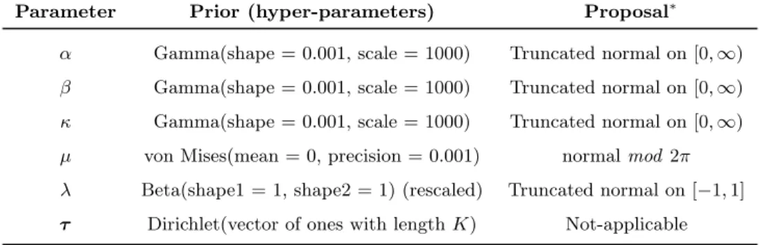
Table 1: Choice of priors and proposal distributions at the input of Algorithm 1
Parameter Prior (hyper-parameters) Proposal∗
α Gamma(shape = 0.001, scale = 1000) Truncated normal on [0,∞) β Gamma(shape = 0.001, scale = 1000) Truncated normal on [0,∞) κ Gamma(shape = 0.001, scale = 1000) Truncated normal on [0,∞) µ von Mises(mean = 0, precision = 0.001) normalmod 2π λ Beta(shape1 = 1, shape2 = 1) (rescaled) Truncated normal on [−1,1]
τ Dirichlet(vector of ones with lengthK) Not-applicable ∗The means of the proposal distributions at each iteration are the draws in the previous iteration
(or the initial component values at the first iteration); the variances of the proposal distributions are adjusted every 50 iterations (see Section 3.2.1 for details.)
To estimate a parameter y ∈ ζ of the target distribution (Abe-Ley in our case) from a set of observations S, MH iteratively refines its estimate yi in
iterationi, starting from an initial valuey0fori= 0. Givenyiin each iteration
i, a new drawy∗ is obtained from a predefined proposal distribution q(y∗|yi).
Then,y∗ is accepted with acceptance probability
A= min 1, p(y ∗|S)q(y(i)|y∗) p(y(i)|S)q(y∗|y(i)) (5)
wherepdenotes the target density.
Finally, the accepted draws are returned as the output of MH algorithm.
Note that, when estimating the components of the mixture models, the MH
algorithm should also estimate the component allocations and weight distribu-tions of each component (τk) in addition to its parameters (ζk) .
Algorithm 1 summarizes our approach, which basically adapts the MH
al-gorithm to estimate the parameters of theK-component Abe-Ley mixture and obtain the component membership of each observation. Similar to the original
MH, the input to our algorithm comprises (i) the target distributions (i.e., the
Abe-Ley mixture model defined by (2)), (ii) the observationsS, with|S|=N, and (iii) the prior and proposal distributions for each parameter. Table 1
pa-Algorithm 1:Metropolis-Hastings
Input :The target distributionf(θ, x|ϑ) with unknown parameter
vectorϑ(defined by (2)); data samplesS with|S|=N; priors and proposal distributions for each parameter inϑ(see Table 1)
Output:the draws forϑ (i.e.,ϑi); the allocation vectorl= (l1, . . . , lN)
/* l denotes to which component each of the observations are assigned (if (θn, xn) is part of component k, then ln=k) */ 1 Initializeϑ0= (ζ01, . . . ,ζK0,τ0) andl0;/* allocate samples in S to
each component with probability τ0
to obtain l0
*/
2 foreachi= 0, . . . , M0+M −1do
/* Given li, estimate the mixture parameters */
3 foreachk= 1, . . . , K do
4 foreachy∈ζk do
/* update parameters of each component in this loop */
5 Sample the component parametery∗ from a proposal
distributiony∗∼q(y∗|y(i));
6 Sampleufrom a Uniform distribution on [0,1]; 7 Calculate the acceptance ratio asA= min{1, p(y
∗)q(y(i)|y∗) p(y(i))q(y∗|y(i))}; 8 y(i+1)= y∗ u < A y(i+1) u≥A
9 Classify each observation (θn, xn)∈S conditional on knowing ζi1, . . . ,ζiK, by samplingln independently for eachn= 1, . . . , N
from: p ln=k|ζi1, . . . ,ζ i
K,(θn, xn)∝p (θn, xn)|ζik
to obtainli;
10 Sampleτi= (τ1i, . . . , τKi) from the Dirichlet distribution
D(e1(li), . . . , eK(li)), whereek(li) =e0+Nk(li), k= 1, . . . , K, and
Nk(li) is the number of data points allocated to componentkof the
mixture at iterationiande0is the prior of the Dirichlet distribution;
11 Disregard the firstM0 draws;
rameter of the Abe-Ley distribution. The priors are non-informative (i.e., the
hyper-parameter selection is such that the resulting priors are almost uniform
across the parameter domains). The choices of proposal distributions (used for sampling the new value for parameters) are (truncated) normal distributions
de-fined on the permitted domain of the parameters. The Abe-Ley density function
is used for determining the component allocation in each iteration of the
algo-rithm. The output of the algorithm comprises draws for the parameter vector
ϑand the allocation vectorl= (l1, . . . , lN) that indicates to which component
each observation belongs.
Algorithm 1 starts by randomly initializing the component parameters on
their permitted domains to obtain ϑ0 = (ζ01, . . . ,ζ0K,τ0) and assigns each ob-servation (θn, xn)∈S to a component with probabilityτ0 to obtain the initial
allocation vector l0 (Line 1). The algorithm then runs for (M0+M)
itera-tions, whereM0is the number of initial samples to disregard (burn-in samples).
Each iteration consists of two parts. In the first part (Lines 3-8), the parameters
ζi1, . . . ,ζiKof each component of the mixture are drawn using the MH algorithm: for each component, new parameter values are sampled from the proposal
distri-butions defined in Table 1 (Line 5) and are accepted with probabilityAdefined by (5) (Line 8).
In the second part of the iteration, the allocation vector l and component
weight vectorτ = (τ1, . . . , τK) are sampled (Lines 9-10). To identifyli (the
al-location vector in iterationi), first the probability of each observation (θn, xn)
belonging to a component k of the mixture is calculated independently us-ing p((θn, xn)|ζik), where ζ
i
k is the parameter vector of component k drawn
at iteration i. Note that p((θn, xn)|ζik) is an Abe-Ley distribution defined by
(1) and not an Abe-Ley mixture model. In other words, p((θn, xn)|ζik)
de-notes the probability of observation n coming from an Abe-Ley distribution with parametersζik. The observation is then assigned to a component k with probability p((θn, xn)|ζik). (Line 9). Once l
i
is identified, the number of
ob-servations allocated to each component of the mixture is counted to calculate
τi = (τ1i, . . . , τKi) is then sampled from that Dirichlet distribution (Line 10). Finally, the firstM0 draws are discarded andM remaining draws are returned
for (ϑ,l) (lines 11-12).
3.2. Addressing the Challenges of a Bayesian Approach
In this section, we explain how we tackle three computational aspects in our
proposed approach: (1) improving the convergence rate of the MH algorithm
via anadaptive Metropolis-Hastings algorithm, (2) addressing the label switch-ing issue (caused by invariance of the mixture likelihood to a permutation of
component parameters) and (3) Bayesian model selection (for determining the
optimal number of mixture components). Note that the second and third
chal-lenges are inherent to parameter estimation for mixture models in general, both
in Bayesian approaches as well as EM-based methods.
3.2.1. Adaptive Metropolis-Hastings
A crucial factor in developing an efficient MH algorithm is the definition
of the proposal distribution,q y∗|yi
. In most applications, a symmetric,
uni-modal distribution such as the Gaussian distribution is chosen. The MH
al-gorithm requires that the variance of the proposal distribution is preset and
does not change during the execution of the MCMC procedure. However, the
choice of this variance parameter has an important impact on the efficiency of
the MCMC algorithm. When the variance of the proposal distribution is too
large, the acceptance probability (defined by (5)) will tend to 0. As a result,
the Markov Chain will retain its current value and only jump to new values with vanishing small probability. On the other hand, when the variance of the
proposal distribution is too small, the acceptance probability will become close
to 1. In this case, the Markov Chain is constantly sampling new values, but
these values are very close to the current value, and it will take an excessive
amount of time before the entire posterior distribution is sampled.
The variance of the proposal distribution has to be set so that both
from the posterior distribution for some time and then evaluate the acceptance
probabilities. The variances of the proposal distributions should then be
ad-justed in order to achieve an acceptance probability of 0.3−0.5. These values ensure that the algorithm does not output the same value, while still making
reasonably large jumps. However, in the current mixture model, this approach
is difficult to implement. As shown in Algorithm 1, the parameters of each
component of the mixture are sampled in blocks. Each component has five
pa-rameters,ζ= (α, β, µ, κ, λ). In the MH algorithm we have to set a variance for each parameter of theK components, so 5·K in total. Tuning these variances is tedious and time consuming.
To overcome the aforementioned challenge, we use a modified version of the
MH algorithm proposed by Haario et al. [22] that automatically adjusts the
variance of the proposal distribution to maximize efficiency. The basic idea of the adaptive Metropolis-Hastings algorithm is that every R iterations (e.g., R= 50), the acceptance probabilities are calculated and evaluated. Whenever the acceptance probabilities are above (below) some threshold (e.g., 0.44), the variance of the proposal distribution is increased (decreased) with an amount
s= min(0.01,pR/i) for the nextR iterations. At that point, the acceptance probabilities are re-evaluated, and the variances are adjusted again, if necessary.
Note that the adjustment amounts is a function of the current iteration i of the MCMC chain, such that at the beginning of the chain larger adjustments
are possible, while subsequent adjustments are forced to become continuously
smaller.
A detailed description of the adaptive Metropolis-Hastings algorithm and the
implications for the mathematical foundations of the algorithm can be found in
[22].
3.2.2. Label Switching Issue
Note that the likelihood of the K-component mixture model in (2) is in-variant to any permutation of its component indices (which amounts to a total
are chosen for the component parameters), the resulting posterior will also be
invariant toK! permutations in the labeling of the component parameters. In other words, the posterior will have K! symmetric modes. As a result, labels of the components can permute multiple times in subsequent iterations of the
MCMC sampling, resulting in a label switching problem. Since in our Bayesian
approach, that posterior is used (as distribution for component parameters) for
inference of the model parameters, the label switching issue makes such inference
very challenging.
Early attempts to solve the label switching issue focus on proposing
identifia-bility constraints via prior distributions to force a unique labeling (e.g., [19, 23]).
However, as shown by Stephens [24], identifying such constraints is not always
feasible, especially when systematically separating the posterior modes is not
possible. Hence, two categories of relabeling methods are proposed to post-process the MCMC samples: (1) deterministic relabeling methods that find the
optimal permutation in each iteration of the MCMC sampler by minimizing a
loss function (e.g., Stephens’ algorithm [24], the pivotal reordering algorithm
[25, 26], default [27] and iterative versions [28] of algorithms for equivalence
class representatives, data-based algorithms [28]), and (2) probabilistic
relabel-ing methods that treat permutation of the parameters as missrelabel-ing data with
associated uncertainty and estimate its density using an EM type approach
(e.g., [29]).
We refer the interested reader to [30] for an explanation and performance
comparison of the relabeling methods in terms of CPU times as well as to what extent they agree on the component labels. We note that the data-based
re-labeling algorithm [28] performs better in terms of both performance criteria
(as shown in [28, 30]), and hence use it for the relabeling of the samples from
Algorithm 1. The data-based relabeling is based on the key idea that in a
converged MCMC, while the labels of each cluster might change from one
it-eration to the other, the clusters remain almost the same. Leveraging such
minute difference between the clusters of each iteration, one may keep track of
Further details of the relabeling algorithm are outlined in [28, Algorithm 5].
3.2.3. Bayesian Model Selection
In many modeling problems, the number of mixture components is not
known and needs to be identified as a part of the model selection process. Earlier
attempts tried to estimate the true number of components either by calculating the marginal likelihoods (e.g., [31, 32]) or by trans-dimensional MCMC samplers
(e.g., reversible jump MCMC [33]). In recent approaches however, the view of
model selection is changed fromidentifying the true model to finding a useful
model [34]. In the latter case, model usefulness is seen as its predictive ability
for future or unseen data (i.e., out-of-sample prediction accuracy [35]). Vehtari
et al.[36] quantify the out-of-sample prediction accuracy as expected log
point-wise predictive density (elpd). However, since future data is not available, to
calculate elpd, first a log point-wise prediction density (lpd) is calculated using
the observed samples. Here, lpd is an over-estimation of elpd for future data,
which can be corrected with a bias term [35]. The lpd measure is calculated from the posterior samples using leave-one-out cross-validation (LOO-CV) as
lpdLOO-CV= n X i=1 log 1 S S X s=1 p yi|θis ! (6)
where n is the number of observations, S is the number of samples from the posterior,θis is a sample sfrom the posterior samples drawn based on all but observationyi, and p(yi|θis) is the probability of observationyi given posterior
parameterθis.
The above calculations are based on n−1 observations. If n is large, the overestimation is negligible, otherwise it is corrected using a biasbthat denotes the improvement of an estimation whennobservations are considered.
Note that the calculations oflpdLOO-CV are computationally expensive for
a large number of observations. Hence, Vehtariet al.[36] also propose an
effi-cient approximation oflpdLOO-CVusing Pareto-smoothed importance sampling
(PSIS). Still, the approximations by PSIS-LOO are not reliable when the
In that case, 10-fold cross-validation is used to estimate the elpd values as
out-lined in [36, Section 2.3].
For every modeling endeavor there is a trade-off between the interpretability of a model and the predictive performance. Here we focus mainly on the latter,
hence we use elpd values to find the optimum number of mixture components.
To avoid overfitting, we use graphical inspection of the elpd measure’s evolution
for increasing the number of mixture components. We identify a knee point in
that graph as a point beyond which the increase in the number of components
K results in a smaller, or at least not better, elpd value compared to that for smallerK.
4. Validation on a Sample Dataset with Known True Parameters
Before moving to applying our approach to real-world data, we first validate
its capability of correctly estimating the parameters from synthetic samples
generated using a known Abe-Ley mixture model. We generate such data using
the random number generation process explained in Section 2.2. We then run
Algorithm 1 for a total ofM0+M = 100,000 iterations, from which we disregard
theM0= 20,000 initial draws that are considered as burn-in. Additionally, to
reduce auto-correlation between the samples, we use thinning by a factor 5, (i.e., only keeping every 5th draw of the MCMC chain) in Algorithm 1. Hence, we
finally retain 20,000 draws with a burn-in of 5,000 initial samples. The choice
of 5 is based on the auto-correlation plots of the posterior draws.2 We use
trace plots to examine the convergence and mixing performance of an MCMC
chain. As a spread measure of the posterior distribution, we use a 95% Bayesian
credible interval.
The top row of Fig. 1 shows the data sampled from a mixture of three
(dataset (a)) and four (dataset (b)) Abe-Ley distributions along with the true
Abe-Ley mixture densities in the form of contour plots. Both datasets contain
2Note that the auto-correlation plots are excluded from this paper to maintain a reasonable
0 100 200 300 0 2 4 6 Linear axis 0.001 0.002 0.003 0.004 0.005 0.006
Dataset (a) true density
0 100 200 300 400 0 2 4 6 Circular axis Linear axis 0.001 0.002 0.003 0.004 0.005
Dataset (a) estimated density
0 100 200 300 0 2 4 6 0.01 0.02 0.03
Dataset (b) true density
0 100 200 300 0 2 4 6 Circular axis 0.01 0.02 0.03
Dataset (b) estimated density
Fig. 1: Sampled datasets from mixture of true (top row) and estimated (bottom row) Abe-Ley distributions. Contour plots indicate two-dimensional kernel densities
0 5 15 Component 1 density N = 12500 Bandwidth = 0.002754 α 0.94 1.02 0.60 10000 20000 1.2 1.8 Component 1 traceplot 0 4 8 Component 2 density N = 12500 Bandwidth = 0.005205 1.89 2.04 0.50 10000 20000 1.5 Component 2 traceplot 0.0 1.0 2.0 Component 3 density N = 12500 Bandwidth = 0.02493 9.55 10.26 0 10000 20000 2 6 10 Component 3 traceplot 0 40 100 N = 12500 Bandwidth = 0.0003872 β 0.06 0.07 0.00 10000 20000 0.3 0 20 40 N = 12500 Bandwidth = 0.001223 0.19 0.22 0.200 10000 20000 0.35 0 4000 N = 12500 Bandwidth = 7.294e−06 0.0099 0.0101 0.0 0 10000 20000 0.6 0 4 8 12 N = 12500 Bandwidth = 0.004395 κ 0.87 0.99 0.00 10000 20000 1.0 0 4 8 12 N = 12500 Bandwidth = 0.004638 2.90 3.03 0 10000 20000 1.5 2.5 0 4 8 12 N = 12500 Bandwidth = 0.004187 1.92 2.04 0 10000 20000 2 6 0 4 8 N = 12500 Bandwidth = 0.005017 µ −0.08 0.07 0 10000 20000 0.0 1.0 2.0 0 40 100 N = 12500 Bandwidth = 0.0004038 3.13 3.15 0 10000 20000 3.11 3.14 0 20 40 N = 12500 Bandwidth = 0.001149 1.56 1.60 0 10000 20000 1.5 3.0 0 2 4 6 N = 12500 Bandwidth = 0.008324 λ −0.12 0.11 −1.00 10000 20000 −0.2 0 2 4 6 8 N = 12500 Bandwidth = 0.008802 −1.00 −0.76 −1.00 10000 20000 −0.4 0 2 4 6 N = 12500 Bandwidth = 0.008677 0.69 0.94 −1.0 0 10000 20000 0.0 1.0 0 20 40 τ 0.31 0.34 0 10000 20000 0.3 0.5 0.7 0 20 40 0.33 0.36 0.250 10000 20000 0.45 0 20 40 0.32 0.35 0.0 0 10000 20000 0.2
Fig. 2: Posterior densities and trace plots of the parameters for mixture of 3 Abe-Ley (Dataset (a)). Black vertical lines mark the true parameter values and shaded areas are the 95% Bayesian credible intervals
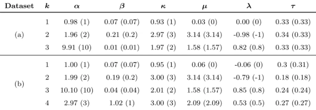
Table 2: Estimated and true parameters for sampled data from mixture of Abe-Ley distribu-tion (The true values are shown in parenthesis)
Dataset k α β κ µ λ τ (a) 1 0.98 (1) 0.07 (0.07) 0.93 (1) 0.03 (0) 0.00 (0) 0.33 (0.33) 2 1.96 (2) 0.21 (0.2) 2.97 (3) 3.14 (3.14) -0.98 (-1) 0.34 (0.33) 3 9.91 (10) 0.01 (0.01) 1.97 (2) 1.58 (1.57) 0.82 (0.8) 0.33 (0.33) (b) 1 1.00 (1) 0.07 (0.07) 0.95 (1) 0.06 (0) -0.06 (0) 0.3 (0.31) 2 1.99 (2) 0.19 (0.2) 3.00 (3) 3.14 (3.14) -0.79 (-1) 0.18 (0.18) 3 10.10 (10) 0.04 (0.04) 2.01 (2) 1.58 (1.57) 0.85 (0.8) 0.24 (0.24) 4 2.97 (3) 1.02 (1) 3.00 (3) 2.09 (2.09) 0.53 (0.5) 0.27 (0.27)
4,500 samples. The number of samples from each component of the mixture is
the same in dataset (a) but different per component in dataset (b) (see
compo-nent weights from Table 2).
As mentioned earlier, one of the defining advantages of the MH algorithm
is that — unlike likelihood-based estimations, which are point estimates — the
MH algorithm outputs samples from the posterior distribution of the model
parameters, making the uncertainty of the estimates directly inferable from
the posterior densities, without the need for extra calculations (such as in boot-strapping). The posterior densities of the parameters for a mixture of 3 Abe-Ley
distributions (dataset (a)) are shown in Fig. 2. The accompanying trace plot
for each parameter is used to analyze the convergence and mixing performance
of the MH algorithm. As seen from the trace plots, the burn-in of 5,000 initial
samples is sufficient to disregard the unstable initial draws of the algorithm.
The retained draws are from the higher probability region of the posterior and
are close to the true values of the parameters, indicating that the chain has
converged. The density plots in Fig. 2 are based on the 15,000 retained draws.
Finally, the trace plots also confirm that the draws among various iterations are not identical: the chain is mixing well and effectively exploring the posterior.
For some parameters however, the mixing of the chain is not apparent: this is
the true value of the parameter. Also, very low auto-correlation is observed
among the draws, which confirms efficient exploration of the posterior.
The shaded regions in the density plots of Fig. 2 indicate the 95% Bayesian credible intervals. The boundaries of the credible intervals are marked with
numeric values on the horizontal axis, while the black vertical lines show the
true values of the parameters. For some parameters, the true values are in the
tails of the posterior. This is only natural, since there is always a 5% chance that
the true value will be outside this credible interval, and we have 5 parameters
per component plus the component weights (in this case totaling 18).
To demonstrate the estimated predictive density for both datasets, we use
the last 4,500 MCMC draws ofϑi and for each draw, sample a data point from the Abe-Ley mixture distribution parameterized by ϑi. The generated data points are composed and presented in Fig. 1. We then use a two-dimensional kernel density estimate to obtain the estimated predictive density (shown in the
form of contour plots in Fig. 1). As seen from Fig. 1, the estimated and true
predictive density of the Abe-Ley mixtures for both datasets are very similar.
This comparison further validates the effectiveness of the proposed approach in
estimating the parameters of the Abe-Ley mixture distributions.
While noting that Bayesian estimation is not a point estimate, still, to be able
to numerically compare the component-wise densities for the true and the
esti-mated parameters, we summarize the posterior distributions in point forms. To
do that, we use maximum a posteriori (MAP) estimation, which corresponds to
the mode of the empirical distribution of the posterior. An alternative summa-rization would be taking the mean of the posterior distribution, but that Bayes
estimate is not suitable for multi-modal posteriors. The true and estimated
pa-rameters we thus obtain are summarized in Table 2. These results indicate that
our proposed algorithm can effectively estimate the mixture model parameters
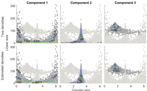
for both datasets. For dataset (a), we further demonstrate component-wise
den-sities for the true and the estimated parameters in Fig. 3. This figure shows
that the true and estimated densities for the mixture of 3 Abe-Ley distributions
Fig. 3: Component-wise densities for the true and the estimated parameters for Dataset (a) 2 3 4 5 -2.95 -2.9 -2.85 -2.8 -2.75 -2.7
Expected log pointwise predictive density
(elpd)
104 Dataset (a)
2 3 4 5 6 7
Number of mixture components -2.7 -2.6 -2.5 -2.4 -2.3 -2.2 -2.1 10 4 Dataset (b)
Fig. 4: Determining number of mixture components using elpd measure for sample datasets (the bend in each curve is used for selecting the best number of mixture components).
To validate the effectiveness in model selection of elpd, approximated by
PSIS-LOO, we have calculated the elpd for a varying number of mixture
com-ponents for both datasets as shown in Fig. 4. The location of the bend (knee)
in Fig. 4 indicates the most suitable number of components, which is the same
as the number of true mixtures for both datasets.
algorithm for estimating the parameters of a mixture of Abe-Ley distributions
and of elpd as suitable model selection measure. Next, we apply our approach
to model the data for two different real-world applications.
5. Modeling Real-World Datasets with a Mixture of Abe-Ley Distri-butions
We now apply our methodology to fit an Abe-Ley mixture to (1) a wave
dynamics dataset, and (2) an EV charging dataset. The first application is a traditional application domain of mixtures of cylindrical distributions where the
circular measurement is the direction (angle). The dataset in the second example
on the other hand is a new one, where the circular measurement is periodic time.
For both applications, we run Algorithm 1 for M0+M = 100,000 iterations
and discard a burn-in ofM0 = 20,000 draws. Further, we use thinning by a
factor 5, i.e., we only keep every 5th draw of the MCMC chain) to reduce the
auto-correlation among subsequent draws.
5.1. Wave Dynamics in the Adriatic Sea
In this section, we consider a dataset of wave dynamics, which is a
well-studied application of the Abe-Ley distribution. The dataset comprises
semi-hourly wave directions and heights in the Adriatic Sea, recorded in the period
15 February 2010 to 16 March 2010 as reported by [11]. Lagonaet al. [11] also
approximate this data with a mixture of Abe-Ley distributions, whose
param-eters depend on the states of a latent Markov chain. However, their proposed estimation algorithm is based on the EM method (and thus a point estimate),
whereas our proposed approximation algorithm is based on the MCMC method
(thus giving a posterior distribution for the mixture parameters). Additionally,
the procedure by Lagona et al. [11] includes a temporal dependence for the
data, based on a hidden Markov model. In this work, we focus on fitting the
distribution only, while addressing temporal dependence could be interesting as
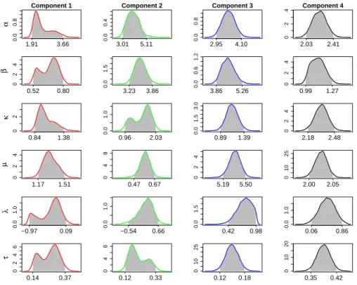
Figure 5 shows the elpd values for different numbers of Abe-Ley mixtures and
suggestsK = 4 as the optimum number of mixtures because the improvement in elpd when increasing the number of mixtures from 2 to 4 is significantly larger than for the increase from 4 to 7 and beyond. Hence,K = 4 is a knee point. Note that in [11] the best number of states (mixtures) is deemed to be
K = 3 using the BIC measure. To represent and compare the distribution of each component of the mixture models, we use MAP estimation to summarize
the estimated parameters from our approach in a point form. The resulting
mixtures are depicted in Fig. 7(b) and are compared with the fits from Lagona
et al.[11] shown in Fig. 7(a).
Figure 7 suggests that both approaches identify similar heterogeneity in the
data. The first component of Lagonaet al.models the high waves coming from
the north [11], which in our model are represented by the first and the second components. The second component of Lagona’s model (and our third
compo-nent) is associated with calm sea and finally, their third component (fourth in
our model) is associated with Sirocco episodes (caused by wind blowing
south-easterly, along the major axis of the Adriatic Sea). However, the posterior
den-sities of the 4 mixture components depicted in Fig. 6 confirm that the Bayesian
approach is more reliable than the EM method. The posterior densities for
component 1 and 2 in Fig. 6 are multi-modal, making the EM based approaches
susceptible to premature convergence to a local maximum.
5.2. Electric Vehicle Hourly Charging Requests
Our second study is motivated by the increasing use of EVs and the need to
analyze their impact on the power grid. Initial studies only presented empirical
distributions of the arrival times of EVs from real-world measurements [37, 38,
39, 40]. Here, we take the first step to model the arrival times of EVs using
2 3 4 5 6 7 Number of mixture components -3700 -3600 -3500 -3400 -3300 -3200
Expected log pointwise predictive density
(elpd)
Fig. 5: The elpd values for model selection in modeling wave dynamics. (The bend in the curve is used for selecting the best number of mixture components.)
0.0 0.8 Component 1 α 1.91 3.66 0.0 0.4 Component 2 3.01 5.11 0.0 0.8 Component 3 2.95 4.10 0 2 4 Component 4 2.03 2.41 0 2 4 β 0.52 0.80 0.0 1.5 3.23 3.86 0.0 0.6 1.2 3.86 5.26 0 2 4 0.99 1.27 0 2 κ 0.84 1.38 0.0 1.0 0.96 2.03 0.0 1.5 3.0 0.89 1.39 0 2 4 2.18 2.48 0 2 4 µ 1.17 1.51 0 4 8 0.47 0.67 0 2 4 5.19 5.50 0 10 25 2.00 2.05 0.0 1.0 λ −0.97 0.09 0.0 1.0 −0.54 0.66 0.0 1.5 0.42 0.98 0.0 1.0 0.06 0.86 0 2 4 6 τ 0.14 0.37 0 4 8 0.12 0.33 0 10 25 0.12 0.18 0 10 20 0.35 0.42
Fig. 6: Posterior densities of the parameters for best Abe-Ley mixture model for wave dy-namics.
0 2 4 (b) (a) Component 1 0.05 0.2 0.1 0.25 Component 2 0.6 0.4 0.1 0.3 Component 3 0.6 0.1 0.5 0.1 0 2 4 6 0 2 4 Wave hight (m) Component 1 0.06 0.08 0.16 0.18 0.12 0.02 0 2 4 6 Component 2 0.2 0.5 0.6 0.1 0 2 4 6
Wave direction (rad)
Component 3 0.4 0.2 11.4 0 2 4 6 Component 4 0.2 0.4 0.9 0.9
Fig. 7: Component-wise densities for (a) Abe-Ley mixture model estimated by [11] and (b) Abe-Ley mixture model estimated by our proposed approach.
(collected by ElaadNL3) that includes the arrival times of electric vehicles at
public roadside charging stations across the Netherlands from January to March
2015.
We divide a day into hour-long slots and count the number of EV arrivals in each slot. We also take the mean time-of-arrival of EVs in each slot to
characterize the timing aspect of the measurement. Therefore, the resulting
data points have one linear (number of EV arrivals) and one circular (average
time-of-arrival) measurement and are best represented on a cylinder. Note that
the linear measurements in this dataset are of discrete nature. However, due to
3ElaadNL is the knowledge and innovation center in the field of charging infrastructure in
the Netherlands, providing coordination for the connections of public roadside charging sta-tions to the electricity grid on behalf of 6 participating distribution system operators (DSOs). It also performs technical tests of charging infrastructure, researches and tests smart charging possibilities of EVs, and develops communication protocols for managing EV charging. The EV charging session data is available upon request for non-commercial research purposes, subject to signing an agreement. For more information, please contact Chris Develder (email: [email protected]).
2 3 4 5 6 7 Number of mixture components -1.13 -1.12 -1.11 -1.1 -1.09 -1.08 -1.07 -1.06
Expected log pointwise predictive density
(elpd)
104
Fig. 8: elpd values for model selection in modeling EV arrivals (the bend in the curve is used for selecting the best number of mixture components)
unavailability of the cylindrical distributions that effectively take into account
the cross-correlation of the circular and linear measurements for discrete data, we have modeled this dataset with an Abe-Ley distribution as the best existing
candidate. To prevent over-fitting, we add a random value generated from a
uniform distribution on (0,1) to the EV counts in each slot.
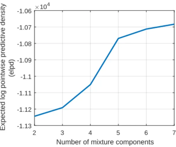
We fit the mixture of Abe-Ley distributions with a varying number of
mix-ture components to the EV dataset and use the elpd measure to select the best
number of mixture components, as illustrated in Fig. 8. The bend in the elpd
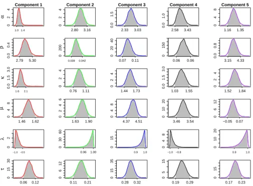
values suggestsK= 5 mixtures to model the EV arrival distribution. The esti-mated posterior densities are shown in Fig. 9, where the shaded regions indicate
the 95% Bayesian credible intervals. We also use MAP estimation to
numeri-cally summarize the posteriors in point forms and show the component densities in Fig. 10.
Next, the resulting mixtures are compared with our previous studies on this
dataset. In [39, 40], we clustered this data on a 2-dimensional surface (i.e.,
time-of-arrival vs. time-of-departure) into 3 clusters: charge-near-work
(charac-terized by early morning arrivals, mainly on weekdays), charge-near-home (with
0 2 4 Component 1 α 1.0 1.4 0 2 4 Component 2 2.80 3.16 0.0 1.5 Component 3 2.33 3.03 0.0 1.0 Component 4 2.58 3.43 0 4 8 Component 5 1.16 1.35 0.0 0.4 β 2.79 5.30 0 200 0.039 0.042 0 20 40 0.07 0.11 0 150 0.06 0.06 0.0 0.8 3.15 4.33 0.0 1.5 3.0 κ 1.6 2.1 0 2 4 0.76 1.11 0 2 4 1.44 1.73 0.0 1.5 3.0 1.03 1.55 0 2 4 1.52 1.84 0 4 8 µ 1.46 1.62 0 2 4 6 1.63 1.90 0 4 8 4.37 4.51 0 10 20 3.46 3.54 0 6 12 −0.05 0.07 0 2 λ −1.0−0.5 0 30 60 0.96 1.00 0 15 0.9 1.0 0 4 8 −1.0 −0.8 0 10 20 0.9 1.0 0 15 30 τ 0.06 0.12 0 6 12 0.11 0.21 0 15 35 0.28 0.32 0 5 15 0.19 0.29 0 15 0.17 0.23
Fig. 9: Posterior densities of the parameters for best Abe-Ley mixture model for EV arrival
We also found that the EV arrivals have different empirical distributions on
weekdays compared to weekends: weekday arrivals have two peaks (mornings and evenings), whereas the weekend arrivals only peak around noon.
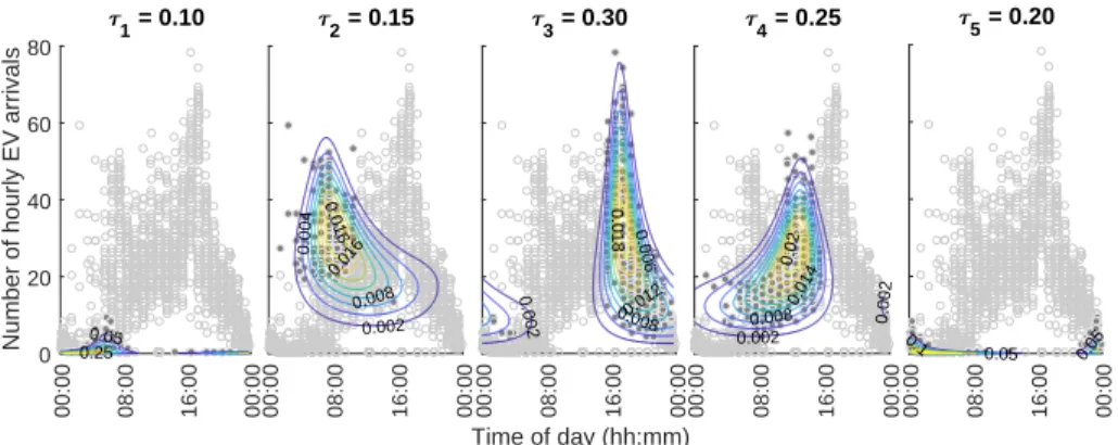
This heterogeneity is very well captured by the mixture of the 5-component
Abe-Ley distribution. As seen in Fig. 10, the second component models the
morning peaks in EV arrivals, which are typically arrivals on weekdays and
from the charge-near-work cluster. The third component of the mixture
com-prises weekday arrivals, from charge-near-home sessions. The fourth component
models the weekend arrivals and day-time charging during the weekdays, which
are typically park-to-charge sessions. Finally, the probability of having a very
small number of EV arrivals is modeled by the first (for very early morning
00:00 08:00 16:00 00:00 0 20 40 60 80
Number of hourly EV arrivals
1 = 0.10 0.05 0.25 00:00 08:00 16:00 00:00 2 = 0.15 0.016 0.016 0.008 0.002 0.004 00:00 08:00 16:00 00:00 Time of day (hh:mm) 3 = 0.30 0.002 0.0080.012 0.018 0.006 00:00 08:00 16:00 00:00 4 = 0.25 0.002 0.008 0.014 0.02 0.002 00:00 08:00 16:00 00:00 5 = 0.20 0.1 0.05 0.05
Fig. 10: Component-wise densities for the true and estimated parameters in modeling EV arrivals
6. Conclusion
In this paper, a Metropolis-Hastings algorithm based on MCMC sampling
was proposed for estimating the components of Abe-Ley mixture models. A
dynamic Metropolis-Hastings algorithm was used to adjust the variance of the
proposal distribution to improve both convergence and exploration of the
pos-terior distribution in the proposed algorithm. Two challenges associated with
estimating the mixture parameters were also tackled: the label switching issue
and the selection of the optimal number of components.
By referring to the posterior distributions of the parameters of the
Abe-Ley mixture, we illustrated that a Bayesian based estimation is more reliable
than EM methods for estimating these parameters, because: (1) the multi–
modality of the posteriors can be inferred directly from the output of the MH
algorithm, hence, local maxima are avoided without a need for additional
calcu-lations (which also do not guarantee arriving at a global optimum), and (2) in
EM-based estimation, the uncertainty of the estimates is not available and
fur-ther calculations are needed to approximate them. While bootstrapping could
address this, in our proposed Bayesian approach, the uncertainty of the
estima-tion is directly inferred from the posteriors.
selection measure by estimating the parameters of actual Abe-Ley mixture
mod-els. Further, we applied our proposed approach to model the data from two
different real-world application domains: wave dynamics and electric vehicle (EV) arrivals. In both applications, the Abe-Ley mixtures captured the data
skewness, the correlation between the circular and linear variables and the data
heterogeneity (multi-modality). We found that the resulting mixtures were
in-tuitively appealing and qualitatively in accordance with previous studies of the
real-world datasets.
Acknowledgements
We thank ElaadNL for providing the data and relevant insights on EV
charg-ing in the Netherlands. Special thanks goes out to Nazir Refa (ElaadNL) for
preparing the raw data for analysis. We also thank Prof. Francesco Lagona
for sharing the wave dynamics data of the Adriatic Sea. Finally, we thank Dr.
Thomas Demeester for his expert advice on the bootstrapping approach.
References
[1] K. V. Mardia, T. W. Sutton, A model for cylindrical variables with
appli-cations, Journal of the Royal Statistical Society. Series B (Methodological)
40 (2) (1978) 229–233.
[2] R. A. Johnson, T. E. Wehrly, Some angular-linear distributions and related
regression models, Journal of the American Statistical Association 73 (363) (1978) 602–606.
[3] S. Kato, K. Shimizu, Dependent models for observations which include
angular ones, Journal of Statistical Planning and Inference 138 (11) (2008)
3538–3549, special Issue in Honor of Junjiro Ogawa (1915 - 2000): Design
of Experiments, Multivariate Analysis and Statistical Inference. doi:10.
[4] S. Sugasawa, K. Shimizu, S. Kato, A flexible family of distributions on the
cylinder, ArXiv e-printsarXiv:1501.06332.
[5] M. Wang, Extensions of probability distributions on torus, cylinder and disc, Ph.D. thesis (2013).
[6] J. J. Fern´andez-Dur´an, Models for circular-linear and circular-circular data
constructed from circular distributions based on nonnegative trigonometric
sums, Biometrics 63 (2) (2007) 579–585.
[7] E. Garc´ıa-Portugu´es, R. M. Crujeiras, W. Gonz´alez-Manteiga, Exploring
wind direction and so2 concentration by circular–linear density
estima-tion, Stochastic Environmental Research and Risk Assessment 27 (5) (2013)
1055–1067. doi:10.1007/s00477-012-0642-5.
[8] J. A. ˜Carnicero, C. Aus´ın, M. Wiper, Non-parametric copulas for
circular-linear and circular-circular data: An application to wind directions,
Stochastic Environmental Research and Risk Assessment 27 (2013) 1991–
2002.
[9] T. Abe, C. Ley, A tractable, parsimonious and flexible model for
cylindri-cal data, with applications, Econometrics and Statistics 4 (Supplement C)
(2017) 91–104. doi:10.1016/j.ecosta.2016.04.001.
[10] T. Abe, A. Pewsey, Sine-skewed circular distributions, Statistical Papers
52 (3) (2011) 683–707. doi:10.1007/s00362-009-0277-x.
[11] F. Lagona, M. Picone, A. Maruotti, A hidden markov model for the analysis
of cylindrical time series, Environmetrics 26 (8) (2015) 534–544, env.2355.
doi:10.1002/env.2355.
[12] F. Lagona, M. Picone, Model-based segmentation of spatial cylindrical
data, Journal of Statistical Computation and Simulation 86 (13) (2016)
[13] M. Ranalli, F. Lagona, M. Picone, E. Zambianchi, Segmentation of sea
current fields by cylindrical hidden markov models: a composite
likeli-hood approach, Journal of the Royal Statistical Society: Series C (Applied Statistics)doi:10.1111/rssc.12240.
[14] J. Bulla, F. Lagona, A. Maruotti, M. Picone, A multivariate hidden markov
model for the identification of sea regimes from incomplete skewed and
circular time series, Journal of Agricultural, Biological, and Environmental
Statistics 17 (4) (2012) 544–567. doi:10.1007/s13253-012-0110-1.
[15] Y. Tang, J. Fu, W. Liu, A. Xu, Bayesian analysis of repairable systems with
modulated power law process, Applied Mathematical Modelling 44
(Sup-plement C) (2017) 357–373. doi:10.1016/j.apm.2017.01.067.
[16] S. Ali, Mixture of the inverse rayleigh distribution: Properties and esti-mation in a bayesian framework, Applied Mathematical Modelling 39 (2)
(2015) 515–530. doi:10.1016/j.apm.2014.05.039.
[17] R. McVinish, K. Mengersen, Semiparametric bayesian circular statistics,
Computational Statistics & Data Analysis 52 (10) (2008) 4722–4730. doi:
10.1016/j.csda.2008.03.016.
[18] G. Nu˜nez-Antonio, E. Guti´errez-Pe˜na, G. Escarela, A bayesian regression
model for circular data based on the projected normal distribution,
Statisti-cal Modelling 11 (3) (2011) 185–201. doi:10.1177/1471082X1001100301.
[19] S. Fr¨uhwirth-Schnatter, Markov chain monte carlo estimation of classical
and dynamic switching and mixture models, Journal of the American
Sta-tistical Association 96 (453) (2001) 194–209.
[20] J. Diebolt, C. P. Robert, Estimation of finite mixture distributions through
bayesian sampling, Journal of the Royal Statistical Society. Series B
[21] G. O. Roberts, A. Gelman, W. R. Gilks, Weak convergence and optimal
scaling of random walk metropolis algorithms, Ann. Appl. Probab. 7 (1)
(1997) 110–120. doi:10.1214/aoap/1034625254.
[22] H. Haario, E. Saksman, J. Tamminen, An adaptive metropolis algorithm,
Bernoulli 7 (2) (2001) 223–242.
[23] S. Richardson, P. J. Green, On bayesian analysis of mixtures with an
un-known number of components (with discussion), Journal of the Royal
Sta-tistical Society: Series B (StaSta-tistical Methodology) 59 (4) (1997) 731–792.
doi:10.1111/1467-9868.00095.
[24] M. Stephens, Dealing with label switching in mixture models, Journal of
the Royal Statistical Society: Series B (Statistical Methodology) 62 (4)
(2000) 795–809.
[25] J.-M. Marin, K. Mengersen, C. P. Robert, Bayesian modelling and inference
on mixtures of distributions, Handbook of Statistics 25 (2005) 459–507.
doi:10.1016/S0169-7161(05)25016-2.
[26] J.-M. Marin, C. Robert, Bayesian core: a practical approach to
computa-tional Bayesian statistics, Springer Science & Business Media, 2007.
[27] P. Papastamoulis, G. Iliopoulos, An artificial allocations based solution
to the label switching problem in bayesian analysis of mixtures of
distri-butions, Journal of Computational and Graphical Statistics 19 (2) (2010) 313–331. doi:10.1198/jcgs.2010.09008.
[28] C. E. Rodr´ıguez, S. G. Walker, Label switching in bayesian mixture models:
Deterministic relabeling strategies, Journal of Computational and
Graphi-cal Statistics 23 (1) (2014) 25–45. doi:10.1080/10618600.2012.735624.
[29] M. Sperrin, T. Jaki, E. Wit, Probabilistic relabelling strategies for the label
switching problem in bayesian mixture models, Statistics and Computing
[30] P. Papastamoulis, label.switching: An R package for dealing with the label
switching problem in mcmc outputs, Journal of Statistical Software, Code
Snippets 69 (1) (2016) 1–24. doi:10.18637/jss.v069.c01.
[31] S. Chib, Marginal likelihood from the gibbs output, Journal of the
Ameri-can Statistical Association 90 (432) (1995) 1313–1321.
[32] S. Chib, I. Jeliazkov, Marginal likelihood from the metropolis-hastings
out-put, Journal of the American Statistical Association 96 (453) (2001) 270–
281.
[33] P. J. Green, Reversible jump markov chain monte carlo computation and
bayesian model determination, Biometrika 82 (4) (1995) 711–732.
[34] J. Piironen, A. Vehtari, Comparison of bayesian predictive methods for model selection, Statistics and Computing 27 (3) (2017) 711–735. doi:
10.1007/s11222-016-9649-y.
[35] A. Gelman, J. Hwang, A. Vehtari, Understanding predictive information
criteria for bayesian models, Statistics and Computing 24 (6) (2014) 997–
1016. doi:10.1007/s11222-013-9416-2.
[36] A. Vehtari, A. Gelman, J. Gabry, Practical bayesian model evaluation using
leave-one-out cross-validation and WAIC, Statistics and Computing 27 (5)
(2017) 1413–1432. doi:10.1007/s11222-016-9696-4.
[37] J. Brady, M. O’Mahony, Modelling charging profiles of electric vehicles based on real-world electric vehicle charging data, Sustainable Cities and
Society 26 (2016) 203–216. doi:10.1016/j.scs.2016.06.014.
[38] Y. B. Khoo, C.-H. Wang, P. Paevere, A. Higgins, Statistical modeling of
electric vehicle electricity consumption in the Victorian EV trial, Australia,
Transportation Research Part D: Transport and Environment 32 (2014)
[39] C. Develder, N. Sadeghianpourhamami, M. Strobbe, N. Refa,
Quanti-fying flexibility in EV charging as DR potential: Analysis of two
real-world data sets, in: Proc. 7th IEEE Int. Conf. Smart Grid Communi-cations (SmartGridComm 2016), Sydney, Australia, 2016, pp. 600–605.
doi:10.1109/SmartGridComm.2016.7778827.
[40] N. Sadeghianpourhamami, N. Refa, M. Strobbe, C. Develder, Quantitive
analysis of electric vehicle flexibility: A data-driven approach, International
Journal of Electrical Power and Energy Systems 95 (2018) 451–462. doi:

![Fig. 7: Component-wise densities for (a) Abe-Ley mixture model estimated by [11] and (b) Abe-Ley mixture model estimated by our proposed approach.](https://thumb-us.123doks.com/thumbv2/123dok_us/84606.2509613/24.918.211.694.185.468/component-densities-mixture-estimated-mixture-estimated-proposed-approach.webp)