Asymptotics of orthogonal polynomials for a weight with a
jump on [−1
,
1]
A. Foulqui´e Moreno, A. Mart´ınez-Finkelshtein, and V.L. Sousa∗
Abstract
We consider the orthogonal polynomials on [−1,1] with respect to the weight wc(x) =h(x) (1−x)
α
(1 +x)βΞc(x), α, β >−1,
where his real analytic and strictly positive on [−1,1], and Ξc is a step-like function:
Ξc(x) = 1 for x ∈ [−1,0) and Ξc(x) = c2, c > 0, for x ∈ [0,1]. We obtain strong
uniform asymptotics of the monic orthogonal polynomials in C, as well as first terms of the asymptotic expansion of the main parameters (leading coefficients of the orthonormal polynomials and the recurrence coefficients) as n → ∞. In particular, we prove for wc a conjecture of A. Magnus regarding the asymptotics of the recurrence coefficients.
The main focus is on the local analysis at the origin. We study the asymptotics of the Christoffel-Darboux kernel in a neighborhood of the jump and show that the zeros of the orthogonal polynomials no longer exhibit clock behavior.
For the asymptotic analysis we use the steepest descendent method of Deift and Zhou applied to the non-commutative Riemann-Hilbert problems characterizing the orthogonal polynomials. The local analysis at x= 0 is carried out in terms of confluent hypergeo-metric functions. Incidentally, we establish some properties of these functions that may have an independent interest.
1
Introduction and statement of results
1.1 Introduction
Szeg˝o is the founder of the modern asymptotic theory of orthogonal polynomials on the unit interval for weights wthat satisfy the Szeg˝o condition
1 −1
logw(x) √
1−x2dx >−∞. (1)
For the classical Jacobi weights the asymptotic results both on and away from the interval of orthogonality, as well as at its endpoints, can be derived using multiple identities that these
∗
Corresponding author.
orthogonal polynomials satisfy: the differential equation, the Rodrigues formula, integral representation, etcetera. However, in a general situation the problem is much more difficult. Starting from the 80’s, many new asymptotic results were found for various classes of weights, and the breakthrough was partially motivated by the development of the tools from potential theory and operator theory.
An important new technique for obtaining asymptotics for orthogonal polynomials in all regions of the complex plane is based on the characterization of the orthogonal polynomials by means of a Riemann–Hilbert problem for 2×2 matrix valued functions due to Fokas, Its, and Kitaev [10], combined with the steepest descent method of Deift and Zhou, introduced in [7] and further developed in [2, 6, 9], to mention a few.
A crucial contribution to this method is [14], where the complete asymptotic expansion for the orthogonal polynomials with respect to a Jacobi weight modified by a real analytic and strictly positive function is obtained. However, not much is known in the case when the weight has a jump discontinuity on the interval. So far, the only contribution is [13], where the authors considered an exponential weight on Rwith a jump at the origin, although from
a different perspective of asymptotics of Hankel determinants.
Combining ideas from [13] and [14], we consider polynomials that are orthogonal on a finite interval [−1,1] with respect to a modified Jacobi weight with a jump, namely
wc(x) = (1−x)α(1 +x)βh(x) Ξc(x), x∈[−1,1], (2)
whereα, β >−1 andh(x) is real analytic and strictly positive on [−1,1], and Ξcis a step-like
function, equal to 1 on [−1,0) andc2 >0 on [0,1]. Observe thatw1 is the weight considered
in [14]. The main asymptotic difference between the polynomials orthogonal with respect to
w1andwc, (c6= 1), lies in their behavior near the origin. While in both cases the analysis near
the endpoints of the interval typically involves Bessel functions, only for c6= 1 do confluent hypergeometric functions appear around the origin.
We usePn(x) = Pn(x;wc) to denote the monic polynomial of degree n orthogonal with
respect to the weightwc on [−1,1],
1 −1
Pn(x;wc)xkwc(x)dx= 0, fork= 0,1, . . . , n−1,
and pn(x) =pn(x;wc) to denote the corresponding orthonormal polynomials,
pn(x) =knPn(x),
where kn>0 is the leading coefficient of pn.
The leading term of the asymptotics of polynomialspnandPn(z) (asn→ ∞) for a weight satisfying the Szeg˝o condition (1) (and wc does) and z∈ C\[−1,1] is well known, see [21].
It can be formulated in terms of two functions that will play a relevant role in what follows, and that we introduce here. Namely,
is the conformal map fromC\[−1,1] onto the exterior of the unit circle, with the branch of
√
z2−1 that is analytic in
C\[−1,1] and behaves like z asz → ∞. Furthermore, since the
weight wc on [−1,1] satisfies (1), we can define the so-called Szeg˝o functionD(z) =D(z;wc)
associated withwc, given by
D(z) = exp √ z2−1 2π 1 −1 log√ wc(x) 1−x2 dx z−x ! , forz∈C\[−1,1],
again with √z2−1 > 0 for z > 1 and √1−x2 > 0 on (−1,1). The function D(z) is a
non-zero analytic function on C\[−1,1] such that
D+(x)D−(x) =wc(x), for a.e.x∈(−1,1),
where D+(x) and D−(x) denote the limiting values of D(z) as z approaches x from above
and below, respectively. In particular, by (1), the limit
D∞= lim z→∞D(z) = exp 1 2π 1 −1 log√ wc(x) 1−x2 dx
exists and is a positive real number. From Szeg˝o’s theory (see [21]) it follows that 2nPn(z) ϕ(z)n = D∞ D(z;wc) ϕ(z)1/2 √ 2(z2−1)1/4 [1 +o(1)], asn→ ∞, (4)
uniformly on compact subsets of C\[−1,1]. Using the multiplicative property of the Szeg˝o
function, we conclude that in comparison with the case c = 1, for c 6= 1 there is an extra factor, corresponding to the Szeg˝o function of the pure jump Ξc.
In this paper, we give uniform and more precise asymptotic results for the special weights (2). We obtain the first terms of the asymptotic expansions forkn,Pn, andpn, as well as for the coefficientsan and bn in the three-term recurrence relation
Pn+1(z) = (z−bn)Pn(z)−a2nPn−1(z), (5)
satisfied by the monic orthogonal polynomials.
From our analysis we are also able to derive strong asymptotics for the orthogonal poly-nomials in the open interval (−1,1), near the endpoints ±1, and what is most interesting, in a neighborhood of the origin where the jump of the weight takes place.
Since the behavior of the polynomialsPn away from the origin is very similar to the case c = 1 treated in [14], we will not present all formulas here. However, all the ingredients are contained in the results of the steepest descent analysis performed in Section 2, so that an interested reader can effortlessly derive the omitted asymptotic formulas. In this paper we concentrate on the features of the polynomials and their coefficients that stem from the discontinuity of the weight at the origin.
1.2 Asymptotics away from the interval of orthogonality
In order to formulate our results we need to introduce some notation. For h(x) real analytic and strictly positive on [−1,1], n∈Nand c >0 we define the following real-valued function and real quantities:
~(x)def= √ 1−x2 2π 1 −1 logh(t) √ 1−t2 dt t−x, x∈(−1,1), (6) ηn=ηn(c) def = logc π log(4n) + nπ 2 + β−α 4 π+~(0), (7)
where is the integral understood in terms of its principal value. In general, we assume always √1−x2>0 forx∈(−1,1), unless stated otherwise.
We also introduce what will play the role of the main phase shift in all asymptotic for-mulas, θn= ( θn(c) def = 2ηn−arg Γilogπc, ifc6= 1, 2 ηn+π2 , ifc= 1, (8)
where Γ(·) is the Gamma function; for purely imaginary values ofλ6= 0, we take arg(Γ(λ))∈ (−π/2, π/2).
The simplest asymptotic result concerns the monic orthogonal polynomialsPn. Observe that a full asymptotic expansion for the usual Jacobi polynomials (h ≡ 1, c = 1) can be found in [21, Theorem 8.21.9], while for general real analytic and positiveh (but withc= 1) it was established in [14]. Here we find only the first two terms of the asymptotic expansion, improving (4):
Theorem 1 We have that 2nPn(z) ϕ(z)n = D∞ D(z;wc) ϕ(z)1/2 √ 2(z2−1)1/4 1 +Hn(z) n +O 1 n2 , as n→ ∞,
uniformly on compact subsets of C\[−1,1]. The functionH(z) is analytic onC\[−1,1], and
given by Hn(z) =− 4α2−1 8(ϕ(z)−1)+ 4β2−1 8(ϕ(z) + 1)− log(c) 2πzϕ(z)
cos(θn)ϕ(z) + sin(θn)−log(c)
π
, (9) with θn defined in (8).
Remark 2 A more detailed analysis of the Szeg˝o function D(·;wc) is carried out in Section
2.3. We can simplify notation in the formula above observing that (z2−1)1/4
is the Szeg˝o function for the weight√1−x2 on [−1,1], and it takes the value 2−1/2at infinity. Hence, D∞ D(z;wc) ϕ(z)1/2 √ 2(z2−1)1/4 = D(∞;wcb ) D(z;wcb ) , where wbc(x) = √ 1−x2w
c(x) is known as the trigonometric weight associated towc.
The RH analysis performed below for z /∈ [−1,1] allows also to establish a result for some relevant parameters associated with the orthogonal polynomials. Recall that the monic polynomials Pn satisfy the three term recurrence relation (5). The asymptotic behavior of
these recurrence coefficients (as n→ ∞) is given in the following theorem:
Theorem 3 Asn→ ∞, an= 1 2 − logc 2πn sin(θn) +O 1 n2 , (10) bn=−logc πn cos (θn) +O 1 n2 , (11) with θn defined in (8).
Remark 4 In [17], A. Magnus studied weights of the form
(1−x)α(1 +x)β|x0−x|γ×
(
B, forx∈[−1, x0) , A, forx∈[x0,1] ,
with A and B > 0 and α, β and γ > −1, and x0 ∈ (−1,1). Formulas (10)–(11) show that
for γ = x0 = 0 the asymptotic behavior of the recurrence coefficients conjectured in [17] is
correct, with the possibility to replaceo(1/n) by O(1/n2) in the error term. For more details see Section 3.2 below; the proof of the conjecture in its full generality is contained in [11].
The leading coefficientsknof the orthonormal polynomialspnsatisfy the following
asymp-totic relation: Theorem 5 Asn→ ∞, kn= 2 n √ πD∞ 1− 2α2+ 2β2−1 8 + log(c) 2π log(c) π + sin(θn+1) 1 n+O 1 n2 , with θn defined in (8).
1.3 Local asymptotics
Now we need to introduce further notation. Set
G(a;ζ)def=1F1(a; 1;ζ)e−ζ/2 =e−ζ/2 ∞ X k=0 (a)k (k!)2 ζ k, (12)
where 1F1(a;b;·) is the confluent hypergeometric function; G is an entire function of ζ for
any value of the parameter a∈C, and G(a; 0) = 1. Furthermore, forx∈(−δ,0)∪(0, δ) let
ρ(x)def= logc π log arcsin(x) 2x 1 +p1−x2 −α+β 2 arcsin(x) +~(x)−~(0), (13) completed to a continuous function on (−1,1) by ρ(0) = 0.
Set also
Υ(c)def= sgn(log(c))
r
2clogc
c2−1, c6= 1, Υ(1) = 1, (14)
where we always take the positive value of the square root. The asymptotic behavior of Pn
on compact subsets of an interval (−δ, δ)⊂(−1,1) is given by the following theorem:
Theorem 6 For δ ∈ (0,1), locally uniformly on compact subsets of (−δ, δ) the following asymptotic formula holds:
Pn(x) = D∞ 2n−1/2p c w1(x) Υ(c) (1−x2)1/4 ×Re ei(ρ(x)+θn−π−2arcsin(x))G(λ; 2inarcsin (x)) 1 +Rn(x) n +O 1 n2 , with Rn(x) =− 4α2−1 8(eiarccos(x)−1)+ 4β2−1 8(eiarccos(x)+ 1) − log(c) 2πxeiarccos(x)
cos(θn)eiarccos(x)+ sin(θn)−
log(c) π + ilogc 2πarcsin(x) logc π +e −i(2ρ(x)+θn+arccos(x)) , ρ(x) given in (13), θn in (8), andλ=ilog(c)/π.
Remark 7 The Riemann-Hilbert analysis we perform next gives us an asymptotic expression forPn’s in a small disk of the complex plane centered at the origin, see formula (101) in Section
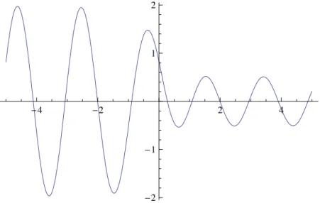
Corollary 8 Locally uniformly forx∈(−δ, δ), δ ∈(0,1), Pn πx n = D∞Υ(c) 2n−1/2p c h(0) Im ei θn/2G(λ; 2πix) 1 +O 1 n , (15)
with θn given in (8) andλ=ilog(c)/π.
See Figure 1 for a typical behavior of the function in the right hand side of (15) close to the origin. !4 !2 2 4 !2 !1 1 2
Figure 1: Typical graphics of the r.h.s. of (15) near the origin.
Recall thatPnhasnsimple zeros, all lying on (−1,1). It is well known that they distribute asymptotically in the weak-* sense according to the equilibrium measure of the interval. In other words, the normalized zero counting measure for the sequence Pn weakly tends to the
absolutely continuous measure on [−1,1] given by ω(x)dx, with
ω(x)def= 1
π
1 √
1−x2.
As it follows from several works of Deift and collaborators (and also from a recent series of papers of Lubinsky and Levin and Lubinsky, see e.g. [15, 16]), a much stronger statement holds: at any point of (−1,0)∪(0,1) they distribute very precisely in accordance withω(x), complying with the so-called “clock behavior”, see e.g. [19]. If, following [19], we enumerate the zerosx(jn) ofPn as follows,
then “clock behavior” at the origin (whereω(0) = 1/π) means lim n→∞ n π xj(n+1) −xj(n)= 1, j ∈Z. (17)
Proposition 9 If c > 1, then the sequence {n x(0n)/π} is dense in an interval of the form [0, t], where t=t(c)<1. Furthermore, 0<lim inf n n π x(kn)−x(k−n)1 ≤lim sup n n π x(kn)−x(k−n)1 <1, k∈N, and lim inf n n π x(kn)−x(k−n)1 >1, −k∈N.
In particular, the clock behavior of the zeros of Pn at the origin does not hold.
If 0< c <1, the same inequalities hold inverting the roles of kand −k.
This result is not surprising, taking into account that x= 0 is not even a Lebesgue point for the weightwc, that is, regardless of the meaning we give towc(0),
lim s→0+ 1 s s −s |wc(x)−wc(0)|dx6= 0.
However, to the best of our knowledge,wcwithc6= 1 provides the first instance of an explicit
orthogonality measure for which the clock behavior fails in the bulk (interior of its support).
Remark 10 A weaker condition than (17) is the quasi-clock behavior (see [19]), namely
lim
n→∞
x(jn+1) −x(jn) x(1n)−x(0n)
= 1, j∈Z.
This limit is violated in our situation too. However, lim j→±∞lim infn→∞ n π x(jn+1) −x(jn)= lim j→±∞lim supn→∞ n π x(jn+1) −x(jn)= 1, (18) which shows a smooth transition to the genuine clock behavior as we move away from the jump of the weight.
Very much related with the clock behavior is the “universality problem” for the Christoffel-Darboux (or CD) kernel
Kn(x, y)def=
n−1
X
k=0
pk(x)pk(y), (19)
where pn are the orthonormal polynomials with respect to the weight wc. This problem
many researchers. A recent series of remarkable contributions of Lubinsky allowed to weaken considerably the conditions on the weight to be able to assure universality: now we know that for twithin the support of the weight where it is continuous,
lim n→∞ π n√1−t2Kn t+ πx n√1−t2, t+ πy n√1−t2 = sin (π(x−y)) π(x−y) . (20) The right hand side is the well-known sine (or sinc) kernel; for our weightwc, this formula is valid for t∈(−1,0)∪(0,1). It was observed in [16] that (20) implies (17).
We show that the jump discontinuity in the weight leads to a different kernel, constructed in terms of the confluent hypergeometric function defined in (12):
Theorem 11 For c >0, c6= 1, locally uniformly forx and y on(−δ, δ), 0< δ <1, lim n→∞ π nKn πx n , πy n =K∞(x, y), (21) with K∞(x, y) = 1 h(0)πi logc c2−1 G(1 +λ; 2πix) ;G(λ; 2πiy) x−y , x6=y, 2 h(0) logc c2−1(G
0(1 +λ; 2πix)G(λ; 2πix)−G(1 +λ; 2πix)G0(λ; 2πix)), x=y,
(22)
where λ = ilog(c)/π, G was introduced in (12), and as usual, [f(x);g(y)] = f(x)g(y) −
f(y)g(x).
Several remarks are in order.
Since G0(1 +λ; 0) = λ+ 1/2 andG(λ; 0) = 1, evaluating K∞(0,0) in (22) we conclude that lim n→∞ Kn πxn ,πxn Kn(0,0)
=G0(1 +λ; 2πix)G(λ; 2πix)−G(1 +λ; 2πix)G0(λ; 2πix),
locally uniformly in (−δ, δ). This shows that even the weak Lubinsky’s “wiggle condition” (term coined by B. Simon, see e.g. [19, Theorem 3.6]) is not satisfied in a neighborhood of the jump of the weight.
The kernel for x 6= y in (22) is written in the so-called integrable form. Taking into account the properties of the functions in the right hand side, we can rewrite it alternatively in a totally real form:
K∞(x, y) = 2
π(x−y)h(0) logc
SinceG(1, z) = exp(z/2), straightforward computations show that asc→1,K∞reduces to the sine kernel. Notice that combining ideas from [16] and [18] we can use (23) to arrive at the same conclusions about the spacing of zeros ofPn’s as we did at the end of Subsection
3.4.
The confluent hypergeometric functions appeared in the scaling limit (as the number of particles goes to infinity) of the correlation functions of the pseudo-Jacobi ensemble in [3]. This ensemble corresponds to a sequence of weights of the form
(1 +x2)−n−Re(s)e2 Im(s) arg(1+ix), x∈R, (24) wherenis the degree of the polynomial andsis a complex parameter. The connection between both problems becomes apparent if we perform the inversionx7→1/xin (24); this creates at the origin an algebraic singularity with the exponent Re(s) and a jump depending on Im(s).
K∞ is a particular case of the reproducing kernel obtained by Borodin and Olshansky in Theorem 2.1 of [3] when Re(s) = 0; for a general situation, see [11].
A recent paper of Lubinsky [15] revealed an interesting connection ofK∞with the theory of entire functions. Namely, in accordance with Theorem 1.6 of [15], K∞ is a reproducing kernel of a de Brange space, equivalent to a classical Paley-Wiener space. More precisely and following the notation of [15], the Hermite-Biehler class HB is the set of entire functions
E with no zeros in the upper half plane C+ def= {Imz > 0} and such that |E(z)| ≥ |E(z)|
for z ∈ C+. The de Branges space H(E) corresponding to E ∈ HB is comprised of entire
functions g such that both g(z)/E(z) and g(z)/E(z) belong to the Hardy class H2(C+). A
reproducing kernel for H(E) is K(x, y) = i
2π
E(x)E(y)−E(x)E(y)
x−y , x6=y. (25)
Comparing this expression with K∞ in (22) we conclude that K(x, y) =K∞(x, y),
with λ=ilog(c)/π and
E(z) = 2 h(0) logc c2−1 1/2 G(λ,2πiz)∈HB
(see below). Lubinsky showed that reproducing kernels, different from the right hand side in (20), can appear for sequences of measures (cf. [3]). To the best of our knowledge, this is the first explicit example of a non-sine reproducing kernel of a de Brange space that arises as a universality limit in the bulk of a fixed measure of orthogonality.
The proof of the asymptotic results stated in this paper (see Section 3) is based on the steepest descent analysis of the Riemann-Hilbert problem that we carry out in Section 2. A key step is the construction of the local representation at the origin, which is done in
Subsection 2.6. The study of the zeros ofPn’s at the origin, the analysis of the clock behavior and the connection with the de Brange spaces requires some further properties of the confluent hypergeometric function1F1(λ; 1;z), which we were unable to find in the literature and which
might have an independent interest. We summarize them in the next proposition; the proofs are relegated to Section 4.
Proposition 12 Let a∈R\ {0}. Then
(i) functions
f1(z) =G(ia, iz) and f2(z) =G(1 +ia, iz)
(see (12)) belong to the Hermite-Biehler class HB; (ii) forx∈R,
1F1(ia; 1;ix)6= 0 and 1F1(1 +ia; 1;ix)6= 0. (26)
In particular, all zeros of 1F1(ia; 1;iz) lie in the lower half plane C− def
= {Imz < 0}, while the zeros of 1F1(1 +ia; 1;iz) lie in the upper half plane C+. Additionally,
|1F1(1 +ia; 1;iz)| ≤ |1F1(ia; 1;iz)|, Imz≥0, (27)
and the equality holds only for z∈R. (iii) ifa >0, the function
y(x)def= arg1F1(ia; 1;ix), y(0) = 0,
is real-analytic and non-positive, strictly increasing on the negative and strictly decreas-ing on the positive semiaxis. For a < 0 the same assertion is valid replacing y(x) by −y(x). It is also the solution of the following initial value problem:
xy0 =a(cos (x−2y)−1), y(0) = 0; (28)
(iv) for a∈R, the function
G(x)def=x−2 arg (1F1(ia; 1;ix)) =x−2y(x), G(0) = 0, (29)
is strictly increasing in R.
Remark 13 The assertion in (i) does not imply that 1F1(ia; 1;iz) ∈ HB, and in general,
this is not true.
Interestingly enough, the proof of (i) is based on some properties of the Christoffel-Darboux kernel observed by Lubinsky in [15]. In this sense, the theory of the confluent hypergeometric functions has benefited from the properties of the reproducing kernels. In the opposite direction, the strict inequality in (27) implies that K∞(z, z) >0 for z∈ C\R and c6= 1, see (113) below.
2
The steepest descent analysis
2.1 The Riemann-Hilbert problem
Following Fokas, Its and Kitaev [10] we characterize both the orthogonal polynomials and the CD kernel in terms of the unique solution Y of the following 2×2 matrix valued Riemann-Hilbert (RH) problem: forn∈N,
(Y1) Y is analytic in C\[−1,1].
(Y2) On (−1,0)∪(0,1), Y possesses continuous boundary values Y+ (from the upper half plane) and Y− (from the lower half plane), and
Y+(x) =Y−(x) 1 wc(x) 0 1 . (Y3) Asz→ ∞, Y(z) = I+O 1 z zn 0 0 z−n ,
whereI is the identity 2×2 matrix.
(Y4) Y has the following asymptotic behavior at the end points of the interval: for ζ ∈ {−1,1}set s=α ifζ = 1, and s=β ifζ =−1. Then forz→ζ,z∈C\[−1,1],
Y(z) = O 1 |z−ζ| s 1 |z−ζ|s ! , ifs <0; O 1 log|z−ζ| 1 log|z−ζ| ! , ifs= 0; O 1 1 1 1 ! , ifs >0.
Furthermore, at the originY has the following behavior: for z→0,z∈C\[−1,1],
Y(z) =O 1 log|z| 1 log|z| .
Standard arguments (see e.g. [14]) show that this RH problem has a unique solution given by
Y(z, n) = Pn(z) C(Pnwc) (z) −2πikn−2 1Pn−1(z) −2πik2n−1C(Pn−1wc) (z) , (30)
wherePnis the monic orthogonal polynomial of degreenwith respect towc;knis the leading coefficient of the orthonormal polynomial pn, and C(·) is the Cauchy transform on [−1,1] defined by C(f) (z) = 1 2πi 1 −1 f(x) x−zdx .
Clearly,Yand other matrices introduced hereafter depend onn, fact that we indicate writing
Y(·, n). However, we omit the explicit reference to n from the notation whenever it cannot lead us into confusion.
2.2 First transformations
We apply the Deift-Zhou method of steepest descent to the RH problem above; some of the steps are standard and we occasionally omit those less relevant details that can be easily found in literature (each time we try to provide a suitable reference though). As in (3),
ϕ denotes the conformal mapping from C\[−1,1] onto the exterior of the unit circle. Let
σ3=
1 0
0 −1
be the third Pauli matrix; in what follows, fora∈C\ {0}we use the notation
aσ3 def= a 0 0 1/a ;
then for b∈C,abσ3 is understood as (ab)σ3. Furthermore, if γ is an oriented Jordan arc, and an analytic function f has boundary values atγ, we denote byf+ (resp., f−) its boundary
values on γ from the left (resp., from the right). Set
T(z)def= 2nσ3Y(z)ϕ(z)−nσ3. (31) Then T is the unique solution of the following equivalent RH problem:
(T1) T is analytic in C\[−1,1].
(T2) On (−1,0)∪(0,1), oriented from−1 to 1,Tpossesses continuous boundary valuesT+
and T−, and T+(x) =T−(x) ϕ−+2n(x) wc(x) 0 ϕ2n − (x) . (T3) Asz→ ∞, T(z) =I+O 1 z .
Next transformation is based upon the factorization of the jump matrix forT: ϕ−+2n wc 0 ϕ−−2n = 1 0 w−c1ϕ−−2n 1 0 wc −1/wc 0 1 0 w−c1ϕ−+2n 1 . (32) In order to introduce a contour deformation we need to extend the definition of the weight of orthogonality to a neighborhood of the interval [−1,1].
By assumptions,his a holomorphic function in a neighborhoodU of [−1,1], and positive on this interval. We set
w(z)def=h(z) (1−z)α(1 +z)β (33) holomorphic in U \ ((−∞,−1]∪[1,+∞)), and such that w(x) > 0 for x ∈ (−1,1). In particular,w(0) =h(0). We also extend the definition of the step function Ξc by
Ξc(z) = ( 1, if Rez <0 c2, if Rez≥0. Then we set wc(z)def=w(z) Ξc(z), (34)
which is a holomorphic function in Ue
def
=U \((−∞,−1]∪[1,+∞)∪iR).
With this definition the left and rightmost matrices in (32) have an analytic extension to the portion of Ue in the lower and upper half plane, respectively, and we can define the next
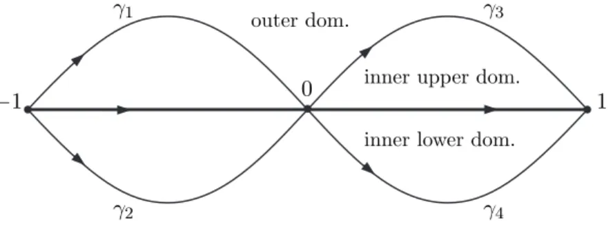
step: lens opening or contour deformation. Namely, we build four new contours γi lying in
−1 0 1
γ1
γ2
γ3
γ4
inner lower dom. inner upper dom. outer dom.
Figure 2: First lens opening.
e
U (except for their end points) such thatγ1 and γ3 are in the upper half plane, and γ1 and γ2 are in the left half plane, and oriented “from −1 to 1” (see Fig. 2). This construction
defines three domains: the inner upper domain, bounded by [−1,1] and the curvesγ1 andγ3;
the inner lower domain, bounded by [−1,1] and the curves γ2 and γ4, and finally the outer
Using the matrixT from (31) we define the new matrixS by S(z)def=
T(z), forz in the outer domain,
T(z) 1 0
−w1
c(z)ϕ
−2n(z) 1 !
, forz in the inner upper domain,
T(z) 1 1 0
wc(z)ϕ
−2n(z) 1 !
, forz in the inner lower domain.
(35)
Then S is the unique solution of the following RH problem: (S1) S is analytic in C\Σ, where Σdef= [−1,1]∪S4i=1γi.
(S2) S satisfies the following jump relations:
S+(z) =S−(z) 1 0 1 wc(z)ϕ(z) −2n 1 ! , forz∈ 4 [ i=1 γi ! \ {−1,0,1}, S+(x) =S−(x) 0 wc(x) − 1 wc(x) 0 , forx∈(−1,0)∪(0,1). (S3) Asz→ ∞, S(z) =I+O 1 z .
(S4) Shas the following asymptotic behavior at the end points of the interval: forζ ∈ {−1,1} set s=α ifζ = 1, ands=β ifζ =−1. Then for z→ζ,z∈C\Σ,
• fors <0: S(z) =O 1 |z−ζ|s 1 |z−ζ|s , asz→ζ; • fors= 0: S(z) =O log|z−ζ| log|z−ζ| log|z−ζ| log|z−ζ| , asz→ζ; • fors >0: S(z) = O 1 1 1 1 !
, asz→ζ from the outer domain;
O |z−ζ|
−s
1 |z−ζ|−s 1
!
(S5) S has the following behavior at the origin: asz→0,z∈C\Σ, S(z) = O 1 log|z| 1 log|z| !
, asz→0 from the outer domain;
O log|z| log|z| log|z| log|z|
!
, asz→0 from the inner domains.
2.3 The Szeg˝o function for wc
In this section we analyze in detail the structure and properties of the Szeg˝o function in-troduced in Section 1.1. Recall that for a non-negative function h on (−1,1) satisfying the
Szeg˝o condition 1 −1 logh(t) √ 1−t2 dt >−∞,
we define in C\[−1,1] its Szeg˝o functionD(·, h) by
D(z, h)def= exp √ z2−1 2π 1 −1 logh(t) √ 1−t2 dt z−t ! = exp p 1−z2C logh(t) √ 1−t2 (z) , (36) with (√1−z2)
+ >0 for z∈(−1,1) in the rightmost expression in (36).
Due to the multiplicative property of the Szeg˝o function, we have that forwc defined in
(33),
D(z, wc) =D(z, w)D(z,Ξc). (37)
Straightforward computation shows that
D(z, w) =D(z, h)(z−1) α/2(z+ 1)β/2 ϕα+2β(z) , D(z,Ξc) =c exp −λlog 1−i√z2−1 z !! , (38) where D(·, h) is computed by formula (36), and
λdef= ilogc
π . (39)
We must clarify that in (38) we take the main branches of (z−1)α/2, (z+ 1)β/2 and√z2−1
that are positive for z >1, as well as the main branch of the logarithm. From (37) we obtain that
D∞def=D(∞, wc) =
√
c D(∞, h) 2−(α+β)/2>0. (40) Let us study the boundary behavior of the Szeg˝o function on the interval. By (38),
lim z→x∈(−1,1), Imz>0 D(z, w) =eπiα/2(1−x)α/2(1 +x)β/2ϕ− α+β 2 + (x) lim z→x∈(−1,1), Imz>0 D(z, h),
where
ϕ+(x) =x+i
p
1−x2 =eiarccos(x), (41)
with (1−x)α/2, (1 +x)β/2 and √1−x2 positive forx∈(−1,1).
Analogously, lim z→x∈(−1,1), Imz<0 D(z, w) =e−πiα/2(1−x)α/2(1 +x)β/2ϕ α+β 2 + (x) lim z→x∈(−1,1), Imz<0 D(z, h).
We can be more specific about the limit values of D(z, h) on (−1,1) if we use the Sokhotskii-Plemelj formulas [12, Section 4.2]:
C± logh(t) √ 1−t2 (z) =±1 2 logh(t) √ 1−t2 + 1 2πi 1 −1 logh(t) √ 1−t2 dt t−x,
where is the integral understood in terms of its principal value. So, if we define~(x) as in
(6), then using (36) we get
lim z→x∈(−1,1), Imz>0 D(z, h) =ph(x)e−i~(x), lim z→x∈(−1,1), Imz<0 D(z, h) =ph(x)ei~(x).
Observe that ~(x) is real-valued on (−1,1), so thate±i~(x)
= 1. So, if we define on (−1,1)
the real-valued function
Φ(x)def= πα 2 − α+β 2 arccos(x)−~(x), (42) then lim z→x∈(−1,1), ±Imz>0 D(z, w) =pw(x) exp (±iΦ(x)).
On the other hand, it is easy to check that with the specified selection of the branch of the square root,
z7→ 1−i √
z2−1 z
is a conformal mapping of C\[−1,1] onto the lower half plane, such that the lower shore of
(−1,1) is mapped onto itself, while the upper boundary is mapped onto (−∞,−1)∪(1,∞). In particular, lim z→x∈(0,1), Imz6=0 arg 1−i √ z2−1 z ! = 0, lim z→x∈(−1,0), Imz6=0 arg 1−i √ z2−1 z ! =−π.
Hence, lim z→x∈(0,1), ±Imz>0 D(z,Ξc) =cexp −λlog 1±√1−x2 x ! =c exp ∓λlog 1 +√1−x2 x ! ,
with √1−x2>0 on (−1,1). Taking into account thate−λπi =c, we also get
lim z→x∈(−1,0), ±Imz>0 D(z,Ξc) = exp −λlog 1±√1−x2 x ! = exp ∓λlog 1 +√1−x2 x ! .
Both identities can be summarized by lim z→x∈(−1,0)∪(0,1), ±Imz>0 D(z,Ξc) = p Ξc(x) exp ∓i logc π log 1 +√1−x2 x ! .
In order to clarify the local behavior of D(z,Ξc) at the origin we observe that for z ∈
C\(−∞,1] functionD(z,Ξc) coincides with cexp
−λlog(1−ipz2−1) +λlog(z),
if we take there the main branch of log(z), so that
e−λlog(z)D(z,Ξc) =c exp −λlog1−ipz2−1. Since lim z→0, Imz>0 log1−ipz2−1= log(2), it yields D(z,Ξc) =c1+ i πlog(z/2)(1 +o(1)), asz→0, Imz >0.
The case Imz <0 can be deduced using the symmetry of D(·, wc) with respect toR.
We can summarize our findings in the following lemma:
Lemma 14 The Szeg˝o functionD(·, w)for the weightwdefined in (33)exhibits the following boundary behavior:
lim
z→x∈(−1,1), ±Imz>0
D(z, w) =pw(x) exp (±iΦ(x)), (43)
with the notation introduced in (6)and (42). Furthermore, for the step function Ξc,
lim z→x∈(−1,0)∪(0,1), ±Imz>0 D(z,Ξc) = p Ξc(x) exp ∓i logc π log 1 +√1−x2 x ! , and D(z,Ξc) =c1± i π log(z/2)(1 +o(1)), as z→0, ±Imz >0. (44)
Obviously, the boundary behavior of the Szeg˝o function D(·, wc) at (−1,1) can be deduced from this Lemma and (37).
2.4 Outer parametrix
Since |ϕ(z)|>1 forz∈C\[−1,1], the matrix Sintroduced at the end of Subsection 2.2 has jumps across each contourγi that are exponentially close toI, as long as we stay away from
the singularities ±1 and 0. So, we can expectS to behave similarly to the 2×2 solution N
of the following RH problem in this region. (N1) Nis analytic in C\[−1,1];
(N2) Nsatisfies the following jump relations on (−1,0)∪(0,1):
N+(x) =N−(x) 0 wc(x) −wc(x)−1 0 ; (N3) Asz→ ∞, N(z) =I+O 1 z .
An explicit solution of this problem is well-known (see e.g. [8] and [14, Section 5]) and can be built in terms of the Szeg˝o function D(·, wc) and its value at infinity defined in (40):
N(z)def=Dσ3 ∞A(z)D(z, wc) −σ3, (45) where A(z)def= A11 A12 −A12 A11 = a(z)+a−1(z) 2 a(z)−a−1(z) 2i a(z)−a−1(z) −2i a(z)+a−1(z) 2 ! , a(z)def= (z−1)1/4 (z+1)1/4, (46)
and we take the principal branches in such a way thatais analytic inC\[−1,1] witha(z)→1
as z → ∞. For future reference it is convenient to notice that an alternative expression for the entries ofA can be obtained using that
A11(z) = a(z) +a−1(z) 2 = ϕ(z)1/2 √ 2 (z2−1)1/4, A12(z) = a(z)−a−1(z) 2i = iϕ(z)−1/2 √ 2 (z2−1)1/4 = i ϕ(z)A11(z), (47)
where we take again the main branches of the roots.
It is known (see [14]) thatN does not match the behavior of S at the endpoints of the interval [−1,1], requiring a separate analysis there. Moreover, comparing the local condition (S5) for S with the behavior of D(·, wc) at the origin (see (44)) we conclude that a local
2.5 Local parametrices at the endpoints of the interval
We fix aδ∈(0,1/8) and for eachζ ∈ {−1,1}we consider the neighborhoodUζ={z∈C: |z−ζ|< δ}
such that Uζ lies entirely in the domainU of analyticity of h. We construct a 2×2
matrix-valued function Pζ in Uζ\Σ that exhibits the same jumps on Σ∩Uζ and the same local
behavior at z=ζ asS, and that matches the matrixNon the boundary∂Uζ. Namely, (Pζ1) Pζ is holomorphic inUζ\Σ and continuous up to the boundary.
(Pζ2) Pζ satisfies the following jump relations:
Pζ+(z) =Pζ−(z) 1 0 1 wc(z)ϕ(z) −2n 1 ! , forz∈Uζ∩ 4 [ i=1 γi ! \ {ζ}; Pζ+(x) =Pζ−(x) 0 wc(x) −w1 c(x) 0 , forx∈Uζ∩((−1,1)). (Pζ3) As n→ ∞, Pζ(z)N−1(z) =I+O 1 n
uniformly forz∈∂Uζ\Σ.
(Pζ4) Pζ has the following behavior as z → ζ, z ∈ Uζ\Σ: with s= α if ζ = 1 and s= β if ζ =−1, • fors <0, Pζ(z) =O 1 |z−ζ|s 1 |z−ζ|s ; • fors= 0, Pζ(z) =O log|z−ζ| log|z−ζ| log|z−ζ| log|z−ζ| ; • fors >0, Pζ(z) = O 1 1 1 1 !
, asz→ζ from the outer domain;
O |z−ζ|
−s
1 |z−ζ|−s 1
!
, asz→ζ from the inner domain.
2.6 Local parametrix at the origin
We fix aδ ∈(0,1/8) and consider the neighborhoodU0 ={z∈C: |z|< δ}such thatU0 lies
entirely in the domainU of analyticity ofh. We construct a 2×2 matrix-valued functionP0
inU0\Σ that exhibits the same jumps on Σ∩U0 and the same local behavior atz= 0 asS,
and that matches the matrix Non the boundary ∂U0. Namely,
(P01) P0 is holomorphic inU0\Σ and continuous up to the boundary.
(P02) P0 satisfies the following jump relations:
P0+(z) =P0−(z) 1 0 1 wc(z)ϕ(z) −2n 1 ! , forz∈U0∩ 4 [ i=1 γi ! \ {0}; P0+(x) =P0−(x) 0 wc(x) − 1 wc(x) 0 , forx∈U0∩((−1,0)∪(0,1)). (P03) As n→ ∞, P0(z)N−1(z) =I+O 1 n
uniformly forz∈∂U0\Σ.
(P04) P0 has the following behavior asz→0,z∈U0\Σ:
P0(z) = O 1 log|z| 1 log|z| !
, asz→0 from the outer domain;
O log|z| log|z| log|z| log|z|
!
, asz→0 from the inner domain.
We build the solution of this problem in two steps. First we obtain a matrix P(1) that satisfies conditions (P01, P02, P04), and after that, using an additional freedom in the
con-struction, we take care of the matching condition (P03).
Let us define at this point an auxiliary functionW holomorphic inU\((−∞,−1]∪[1,+∞)) given by (see (33))
W(z)def= pc w(z), such that W(x)>0 for x∈(−1,1). (48) Then W (x) = (p wc(x)c, −1< x <0; p wc(x)c−1, 0≤x <1. (49)
We construct the matrix functionP0 in the following form:
where En is an analytic matrix-valued function in U0 (to be determined). Matrix P(1) is
analytic in U0\Σ; using the properties of W and ϕit is easy to show that
P(1)+ (x) =P(1)− (x) 0 1/c −c 0 ! , x∈(−δ,0), 0 c −1/c 0 ! , x∈(0, δ), (51) and P(1)+ (z) =P(1)− (z) 1 0 c 1 ! , z∈(γ1∪γ2)∩U0\ {0}, 1 0 1/c 1 ! , z∈(γ3∪γ4)∩U0\ {0}. (52)
Taking into account that W(z) =O(1) and ϕ(z) =O(1) as z→ 0, we conclude also from (P04) thatP(1) has the following behavior at the origin: asz→0,z∈C\Σ,
P(1)(z) = O 1 log|z| 1 log|z| !
, from the outer domain,
O log|z| log|z| log|z| log|z|
!
, from the inner domain.
(53)
In order to constructP(1) we solve first an auxiliary RH problem on a set ΣΨ
def =S6
j=1Γj
of unbounded oriented straight lines converging at the origin, like in Fig. 3. More precisely, Γ1= n teiπ/2 : t >0o, Γ2 = n te3iπ/4 : t >0o, Γ3 = n te5iπ/4 : t >0o, Γ4= n te3iπ/2: t >0 o , Γ5 = n te−iπ/4 : t >0 o , Γ6 = n teiπ/4: t >0 o .
These lines split the plane into 6 sectors, enumerated anti-clockwise from¬to±as in Fig. 3. We look for a 2×2 matrix valued functionΨ(z), satisfying the following conditions: (Ψ1) Ψis analytic in C\ΣΨ.
(Ψ2) for k= 1, . . . ,6,Ψsatisfies the jump relation Ψ+(ζ) =Ψ−(ζ)Jk on Γk, with J1 = 0 c −1/c 0 , J2 =J6 = 1 0 1/c 1 , J3 =J5 = 1 0 c 1 , J4= 0 1/c −c 0 . (54)
¬ ® ± ° ¯ + − + − + − + − +− +− 0 Γ1 Γ4 Γ3 Γ2 Γ5 Γ6
Figure 3: Auxiliary contours Σψ.
(Ψ3) Ψhas the following behavior as ζ →0:
Ψ(ζ) = O log|ζ| log|ζ| log|ζ| log|ζ| ! , forζ ∈¬∪®∪¯∪±; O 1 log|ζ| 1 log|ζ| ! , asζ ∈∪°.
If we use the notationλ=ilog(c)/πintroduced in (39), then we readily see the connection of the RH problem above with that studied recently in [13]. Following the approach of [13] (with slight modifications), we constructΨexplicitly in terms of the confluent hypergeometric functions
φ(a,1;ζ)def= 1F1(a; 1;ζ) and ψ(a,1;ζ)
def
=ζ−a2F0(a, a;−;−1/ζ),
that form a basis of solutions of the confluent hypergeometric equationζw00+(1−ζ)w0−aw = 0, see [1, formula (13.1.1)]. Namely, let
G(a;ζ)def=φ(a,1;ζ)e−ζ/2, H(a;ζ)def=ψ(a,1;ζ)e−ζ/2.
They are solutions of the confluent equation (see e.g. [1, formula (13.1.35)])
ζw00+w0+ 1 2 − ζ 4−a w= 0; (55)
in fact, G(a;·) is the only entire solution of (55) such that G(a; 0) = 1. Function H(a, ζ) is multivalued, and we take its principal branch in−π
2 <arg (ζ)< 3π
2 . For these values ofζ we
define b Ψ(ζ)def= Γ (1−λ)G(λ;ζ) −H(λ;ζ) Γ (1 +λ)G(1 +λ;ζ) Γ(1+Γ(−λλ))H(1 +λ;ζ) ! . By (Ψ2), if we set Ψ(ζ)def= b Ψ(ζ)J6J1, forζ ∈¬; b Ψ(ζ)J6J1J2, forζ ∈; b Ψ(ζ)J6J1J2J3−1, forζ ∈®; b Ψ(ζ)J5, forζ ∈¯; b Ψ(ζ) forζ ∈°; b Ψ(ζ)J6, forζ ∈±;
then Ψhas the jumps across ΣΨ specified in (Ψ2). Explicitly,
Ψ(ζ) = c −1H(λ;ζ) −Γ(1−λ) Γ(λ) H 1−λ;e −πiζ −c−1 Γ(1+Γ(−λλ))H(1 +λ;ζ) H −λ;e−πiζ ! , ζ ∈¬, (56) Ψ(ζ) = Γ (1−λ)G(λ;ζ) − Γ(1−λ) Γ(λ) H 1−λ;e −πiζ Γ (1 +λ)G(1 +λ;ζ) H −λ,1;e−πiζ ! , ζ ∈, (57) Ψ(ζ) = cH λ;e −2πiζ −Γ(1Γ(−λλ))H 1−λ;e−πiζ −cΓ(1+Γ(−λλ))H 1 +λ;e−2πiζ H −λ;e−πiζ ! , ζ ∈®, (58) Ψ(ζ) = −c Γ(1−λ) Γ(λ) H 1−λ;e πiζ −H(λ;ζ) c H −λ;eπiζ Γ(1+λ) Γ(−λ) H(1 +λ;ζ) ! , ζ ∈¯, (59) Ψ(ζ) = Γ (1−λ)G(λ;ζ) −H(λ;ζ) Γ (1 +λ)G(1 +λ;ζ) Γ(1+Γ(−λλ))H(1 +λ;ζ) ! , ζ ∈°, (60) Ψ(ζ) = −c −1 Γ(1−λ) Γ(λ) H 1−λ;e −πiζ −H(λ;ζ) c−1H −λ;e−πiζ Γ(1+Γ(−λλ))H(1 +λ;ζ) ! , ζ ∈±. (61) Direct verification shows thatΨcoincides, after an appropriate change of parameters and a multiplication from the left by the constant matrix
1/c 0
0 1
,
with the solution of the corresponding RH problem found in [13] (cf. formulas (7.26) and (7.27) therein). In consequence, the matrix-valued functionΨdefined in (56)–(61) solves the RH problem (Ψ1)–(Ψ3); moreover, detΨ≡1.
In order to construct the analytic functionEnin (50) we need to study also the asymptotic
behavior of Ψat infinity. Let us introduce the notation
τλ
def
= Γ(−λ) Γ(λ) . Then for purely imaginary values of λ6= 0,
τλ= Γ(λ)
Γ(λ), |τλ|= 1, τ−λ =τλ. This value is not defined for λ= 0; by continuity, we setτ0 =−1.
Lemma 15 As ζ → ∞, ζ ∈C\ΣΨ, and with the notationλ=ilog(c)/π, we have Ψ(ζ) = I+λ ζ −λ −τλ −1/τλ λ +O 1 |ζ|2 ζ−λσ3e−ζσ3/2 × c−σ3, if π 2 <argζ < 3π 2 ; 0 −1 1 0 ! , if −π2 <argζ < π2, (62)
where we use the main branch of ζ−λ =e−λlogζ with the cut along i
R−.
This result is a direct consequence of formulas (4.60)–(4.63) from [13], and can be obtained by straightforward computation using the asymptotic properties of the confluent hypergeometric functions (see e.g. [1, formulas (13.5.1–2)]). In fact, formulas in [1] give us the complete expansion of Ψ.
Now we are ready to build P(1) as in (50). Recall that ϕ is a conformal mapping from
C\[−1,1] onto the exterior of the unit disk, so we can define in C\Rthe analytic function
f(z)def=
(
πi−2 logϕ(z), for Imz >0,
πi+ 2 logϕ(z), for Imz <0, (63)
where we take the main branch of the logarithm. Using thatϕ+(x)ϕ−(x) = 1 on (−1,1) we
conclude that f+(x) = f−(x) there, so that f is holomorphic in C\((−∞,−1]∪[1,+∞)).
For |z|<1 we have
f(z) = 2iz+1 3iz
3+O z5
, asz→0. (64) Hence, forδ >0 sufficiently small, f is a conformal mapping of U0. Moreover, by (41),
f(x) = 2iarcsin(x), x∈(−1,1), (65)
We can always deform our contoursγi close to z= 0 in such a way that
f(γ1∩U0)⊂Γ3, f(γ2∩U0)⊂Γ5, f(γ3∩U0)⊂Γ2, f(γ4∩U0)⊂Γ6.
With this convention, set
P(1)(z)def=Ψ(nf(z)), z∈U0. (66)
By (Ψ1)–(Ψ3) and (64), this matrix-valued function has the jumps and the local behavior at
z= 0 specified in (51)–(53). Taking into account the definition (63) we get that
enf(z)=enπiϕ∓2n(z), for ±Imz >0. Hence, by Lemma 15, Ψ(nf(z)) = I+ λ nf(z) −λ −τλ −1/τλ λ +O 1 n2 (nf(z))−λσ3i−nσ3 × c−σ3ϕnσ3(z), if Imz >0; 0 −1 1 0 ! ϕnσ3(z), if Imz <0, (67)
where the main branch of [nf(z)]λ is taken with the cut along (−∞,0]. Since [f(z)]λ =|f(z)|λexp −logc π arg (f(z)) ,
straightforward computations show that
[f(x)]λ±=
(
|f(x)|λc−1/2, for 0< x <1,
|f(x)|λc−1/2∓1, for −1< x <0, (68)
where we assume the natural orientation of the interval.
Now we will build the analytic matrix En in (50). In order to comply with condition
(P03) above, we need
En(z)∼N(z)ϕ(z)nσ3W(z)σ3 h
P(1)(z)
i−1
uniformly for z∈∂Uδ\Σ. Taking into account (67), we define
En(z) def =N(z)W(z)σ3× inσ3(nf(z))λσ3cσ3, if Imz >0; i−nσ3(nf(z))−λσ3 0 1 −1 0 ! , if Imz <0. (69)
By construction, En is analytic inU0\R. Furthermore, by (N2) and (49), for x ∈(−δ,0)∪ (0, δ), W (x)−σ3N−1 − (x)N+(x)W(x)σ3 = 0 wc(x)/W2(x) −W2(x)/wc(x) 0 = 0 c±1 −c∓1 0 , for ±Rex >0.
From (68) and (69) it follows that
E−n−1(x)En+(x) =I, forx∈(−δ,0)∪(0, δ).
So, the origin is the only possible isolated singularity of En inU0. Proposition 16 lim z→0En(z) = √ 2 2 D σ3 ∞ 1 1 −1 1 eiηnσ3, with ηn introduced in (7). In particular, En is analytic inU0.
Proof. Since En is analytic in a neighborhood of 0 with an at most algebraic singularity
there, it is sufficient to analyze its limit as z → 0 from the upper half plane. By (44) and (64), lim z→0 Imz>0 D(z,Ξc)f(z)−λ = lim z→0 Imz>0 c1+πi log(z/2)− i πlog(f(z))=c3/24−λ.
On the other hand, by (43) and (48) , lim z→0 Imz>0 D(z, w)W(z)−1 =c−1/2eiΦ(0) =c−1/2 exp iα−β 4 π−i~(0) ,
with Φ given by (42) and ~defined in (6).
Summarizing, lim z→0 Imz>0 D(z, wc)−1W(z)f(z)λ= 4λ c e −iΦ(0). By (45) and (69), if Imz >0, En(z) =D∞σ3A(z)mn(z)σ3, (70) with mn(z)def= W (z)f(z) λ D(z, wc) i nnλc. (71)
Gathering the limits computed above, and using that lim
z→0
Imz>0
a(z) =eπi/4
and the definition of ηn, the statement follows.
Therefore, by construction the matrix-valued functionP0given by (50) satisfies conditions
(P01)–(P04). Moreover, it is easy to check that
detP0(z) = 1 for everyz∈U0\Σ.
2.7 Final transformation
Recall that matrices N and Pζ,ζ ∈ {−1,0,1} have det = 1 in their domains of definition.
We may define
R(z)def=
(
S(z)N−1(z), z∈C\ {Σ∪U−1∪U0∪U1};
S(z)P−ζ1(z), z∈Uζ\Σ, ζ ∈ {−1,0,1}. (72) R is analytic in C\ {Σ∪∂U−1∪∂U0∪∂U1}. In fact, since N matches the jump of S on
(−1,1), and Pζ matches the jumps of S within Uζ, ζ ∈ {−1,0,1}, we conclude that R is
analytic in the complement to the contours ΣR depicted in Fig. 4, with additional possible
singularities at{−1,0,1}. But taking into account (S5) and the local behavior ofPζ at these
points (see (Pζ4)), we conclude that these singularities are removable.
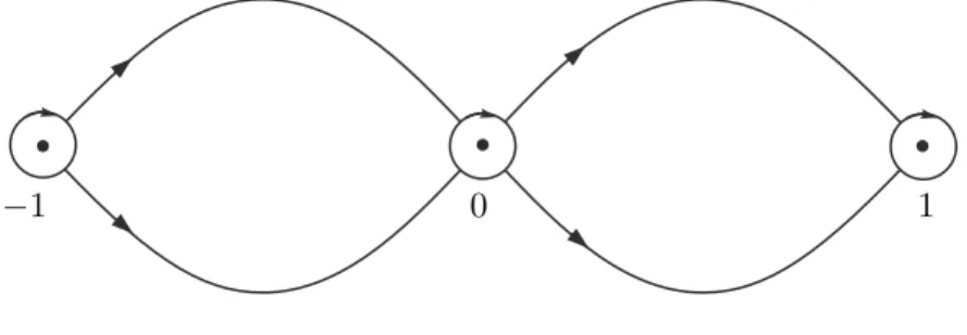
−1 0 1
Figure 4: Contours ΣR.
Now we compute the jumps ofR. For the sake of brevity, we denote ΣoutR def= ΣR\(∂U−1∪∂U0∪∂U1).
Then by (S2) and (72), for z∈Σout R , R+(z) =R−(z)N(z) 1 0 wc(z)−1ϕ(z)−2n 1 N−1(z). (73)
On the other hand, for ∂Uj (j ∈ {−1,0,1}) oriented clockwise, we have that R+(z) =
S+(z)N−1(z) and R−(z) =S−(z)P−j1(z). Hence,
R+(z) =R−(z)Pj(z)N−1(z), z∈∂Uj, j∈ {−1,0,1}. (74)
Summarizing,Rdefined in (72) is analytic inC\ΣR, satisfies the jump relations (73)–(74)
on ΣR, and has the following behavior asz→ ∞: R(z) =I+O 1 z . By (74) and (P03), asn→ ∞, R+(z) =R−(z) I+O 1 n
uniformly on ∂U−1∪∂U0∪∂U1. (75)
On the other hand, there exists a constant 0< q < 1 such that |ϕ(z)|−1 ≤q <1 uniformly on ΣoutR . SinceNdoes not depend on n, we conclude from (73) that asn→ ∞,
R+(z) =R−(z) I+O q2n uniformly on ΣoutR . (76) Motivated by (73) –(76) we define ∆(s)def= N(s) 1 0 wc(s)−1ϕ(s)−2n 1 ! N−1(s)−I, fors∈ΣoutR ; Pζ(s)N−1(s)−I, fors∈∂Uζ, j∈ {−1,0,1},
so that R+(z) =R−(z)(I+∆(z)), z ∈ ΣR. Following [14, Section 8] we can show that ∆
has an asymptotic expansion in powers of 1/n of the form
∆(s)∼ ∞ X k=1 ∆k(s, n) nk , as n→ ∞, uniformly for s∈ΣR. (77) By (76), fork∈N, ∆k(s) = 0, fors∈ΣoutR . (78) Furthermore, by [14, formulas (8.5)–(8.6)], ∆k(s) = (α, k−1) 2k[logϕ(s)]kN(s) h e±iπα2 c 1 2W(s) iσ3 (−1) k k (α2+ 1 2k− 1 4) −(k− 1 2)i (−1)k(k−1 2)i 1 k(α 2+1 2k− 1 4) ! ×he±iπα2 c 1 2W(s) i−σ3
and ∆k(s) = (β, k−1) 2k[log (−ϕ(s))]kN(s) h e∓iπβ2 c− 1 2W(s) iσ3 (−1) k k (β 2+1 2k− 1 4) (k− 1 2)i (−1)k+1(k−1 2)i 1 k(α2+ 1 2k− 1 4) ! ×he∓iπβ2 c− 1 2W(s) i−σ3
N−1(s), for±Ims >0 ands∈∂U−1,
where (α,0)def= 1,
(α, k)def= (4α
2−1)(4α2−9)· · ·(4α2−(2k−1)2)
22kk! .
Each∆kon the small contours encircling±1 is independent ofnand possesses a meromorphic
continuation to U−1 and U1 with the only pole at±1 of order at most [(k+ 1)/2]. However,
unlike in the case analyzed in [14], the existence of a jump in the weight is revealed through the contribution of the local parametrixP0, and hence, each∆kis in general not independent
on n, although uniformly bounded inn.
So, it remains to determine ∆k on ∂U0. Here we calculate explicitly only the first term, ∆1.
Using (45), (48), (50), (63), (67) and (69), we obtain
∆(s) =En(s) λ nf(s) −λ −τλ −1/τλ λ +O 1 n2 E−n1(s), s∈∂U0, n→ ∞. Let us define ∆1(s)def= λ f(s)En(s) −λ −τλ −1/τλ λ E−n1(s), s∈∂U0. (79) Using that by (69), En(s) =F(s) innλσ3 =F(s) incπi logn σ3 , where F(s)def= N(s)W (s)σ3cσ3f(s)λσ3, if Ims >0; N(s)W (s)σ3 0 1 −1 0 ! f(s)λσ3, if Ims <0, we conclude that for s∈∂U0,
∆1(s, n) = λ f(s)F(s) −λ (−1)n+1n2λτλ (−1)n+1n−2λ/τ λ λ F−1(s), (80) which is uniformly bounded in n, so that∆1 in (79)–(80) is genuinely the first coefficient in
Similar analysis can be performed for ∆k(·, n), k≥ 2, taking higher order terms in the
expansion of Ψin (62).
The explicit expression (80) and the local behavior off show that∆1(s, n) has an analytic
continuation toU0except for the origin, where it has a simple pole. Again, a similar conclusion
is valid for other ∆k(s, n), except that now the pole is of order k.
As in [5, Theorem 7.10] we obtain from (77) that
R(z)∼I+ ∞ X j=1 R(j)(z, n) nj , asn→ ∞, (81)
uniformly forz∈C\ {∂U−1∪∂U0∪∂U1}where eachR(j)(z) is analytic, uniformly bounded
inn, and R(j)(z, n) =O 1 z asz→ ∞.
This is a bona fide asymptotic expansion near infinity, since ∀l∈N ∃C >0 :|z| ≥2⇒ R(z)−I− l X j=1 R(j)(z, n) nj ≤ C |z|nl+1,
for any matrix normk·k. The proof is based on the integral representation for R,
R(z) =I+ 1 2πi ΣR R−(s)∆(s, n) s−z ds, z∈C\ΣR
(see [5]); although in our case the coefficients ∆k and Rk in (77) and (81) depend on n,
their uniform boundedness allows to follow the steps of the proof of Lemma 8.3 in [14]. In particular, expanding the jump relationR+=R−(I+∆) up to order 1/n we find that
R(1)+ (s, n)−R(1)− (s, n) =∆1(s, n), fors∈∂U−1∪∂U0∪∂U1.
Since R(1) is analytic in the complement of ∂U−1 ∪∂U0∪∂U1 (see (78)) and vanishes at
infinity, by the Sokhotskii-Plemelj formulas,
R(1)(z, n) = 1 2πi
∂U−1∪∂U0∪∂U1
∆1(s, n) s−z ds.
Recall that∆1can be extended analytically insideUj’s with simple poles at±1 and 0; let us denote by A(1)(n),B(1)(n) and C(1)(n) the residue of ∆1(·, n) at 1, −1 and 0, respectively.
Then residue calculus gives
R(1)(z, n) = A(1)(n) z−1 + B(1)(n) z+ 1 + C(1)(n) z , forz∈C\ {U−1∪U0∪U1}; A(1)(n) z−1 + B(1)(n) z+ 1 + C(1)(n) z −∆1(z, n), forz∈U−1∪U0∪U1. (82)
Residues A(1)(n) and B(1)(n) are in fact independent of n; they have been determined in [14, Section 8]: A(1)(n) =A(1)= 4α 2−1 16 D σ3 ∞ −1 i i 1 D−σ3 ∞ , B(1)(n) =B(1)= 4β 2−1 16 D σ3 ∞ 1 i i −1 D−σ3 ∞ (83)
(notice however an extra factor √c in the constant D∞ with respect to [14]). The value of the remaining residueC(1)(n) is given in the following
Proposition 17 Coefficient C(1)(n) in (82) is given by
C(1)(n) = logc 2π D σ3 ∞ −cosθn λ−isinθn λ+isinθn cosθn D−σ3 ∞ , where θn is defined in (8).
Proof. Taking into account (64) and (79) we conclude that
C(1)(n) = λ 2iEn(0) −λ −τλ −1/τλ λ E−n1(0). By Proposition 16, C(1)(n) = λ 4iD σ3 ∞ 1 1 −1 1 4λe−iΦ(0)innλ σ3 −λ −τλ −1/τλ λ ×4λe−iΦ(0)innλ−σ3 1 −1 1 1 D−σ3 ∞ .
With the notation (7) and choosing ς ∈Rsuch that eiς =τλ, we get 1 1 −1 1 eiηnσ3 −λ −eiς −e−iς λ e−iηnσ3 1 −1 1 1 = 2 −cos(2ηn+ς) λ−isin(2ηn+ς) λ+isin(2ηn+ς) cos(2ηn+ς) .
It remains to observe that 2ηn+ς=θn, and this settles the proof.
3
Asymptotic analysis. Proof of Theorems
Unraveling the transformations Y → T→ S → R we can obtain an expression for Y. We
specify the following domains (see Fig. 5): • De is the unbounded component ofC\ΣR;
• D±i correspond to the portion of the inner domain exterior to Uζ,ζ ∈ {−1,0,1}, lying in the upper (resp., lower) half-plane;
• D±ζ,e is the subset ofUζ in the outer domain and upper (resp., lower) half plane; • D±ζ,i is the subset of Uζ in the inner domain and upper (resp., lower) half plane.
From (31), (35), and (72), Y(z, n) = 2−nσ3RNϕnσ3(z), z∈ D e; 2−nσ3RN 1 0 ±w1 cϕ −2n 1 ! ϕ(z)nσ3, z∈ D i; 2−nσ3RP ζϕ(z)nσ3, z∈ D±ζ,e; 2−nσ3RP ζ 1 0 ±1 wc ϕ −2n 1 ! ϕ(z)nσ3, z∈ D± ζ,i; (84) with ζ∈ {−1,0,1}. −1 1 De Di+ Di− Di+ Di− D+0,e D−0,e D+0,i D−0,i
Figure 5: Domains for Y
Next, using the asymptotic expression forRderived above, we obtain information about the behavior of Y in different domains of the plane.
3.1 Asymptotics for the monic orthogonal polynomials on C\[−1,1]. Proof of Theorem 1.
If K is a compact subset of De, then by (81) and (84),
Y(z, n) = 2−nσ3R(z)N(z)ϕnσ3(z), z∈K. (85) Since Pn(z) =Y11(z, n), we get by (45)–(47) that
2nPn(z)
ϕ(z)n =
D∞
with R(z)def=R11(z)− i D2 ∞ϕ(z) R12(z). (86) By (47) and (81), uniformly on K, 2nPn(z) ϕ(z)n = D∞ D(z, wc) ϕ(z)1/2 √ 2 (z2−1)1/4 1 +Rn(z) n +O 1 n2 , asn→ ∞, with Rn(z)def= R(1) 11(z)− i D2 ∞ϕ(z) R(1) 12(z). (87)
Taking into account the expression for R(1) in (82), as well as (83) and Proposition 17, we
get that R(1)11(z) = 1−4α 2 16(z−1)+ 4β2−1 16(z+ 1)− log(c) cos(θn) 2πz , R(1)12(z) =iD2∞ 4α2−1 16(z−1)+ 4β2−1 16(z+ 1) + log(c) 2π log(c)/π−sin(θn) z . (88)
The trivial identity ϕ2(z) + 1 = 2z ϕ(z) yields 1 z±1 1± 1 ϕ(z) = 2 ϕ(z)±1, (89) and we conclude that in K ⊂ De,Rn(z) =Hn(z), withHn defined in (9).
3.2 Asymptotics of the recurrence coefficients
Recall that monic polynomialsPn satisfy the recurrence relation
Pn+1(x) = (x−bn)Pn(x)−a2nPn−1(x), n= 0,1, . . . ,
with P−1(x) = 0 and an >0. From [10] (see also [8]) it follows that the coefficients can be
found directly in terms of the matrixY in (85):
a2n= lim z→∞z 2Y12(z, n)Y21(z, n) = lim z→∞ −D 2 ∞ 2i +zR12(z, n) zR21(z, n) + 1 2iD2 ∞ , (90) bn= lim z→∞(z−Y11(z, n+ 1)Y22(z, n)) = limz→∞z(1−R11(z, n+ 1)R22(z, n)) . (91)
We may take limits in the asymptotic expansion (81); additionally to (88) we have that R(1)21(z) = i D2 ∞ 4α2−1 16(z−1)+ 4β2−1 16(z+ 1) + log(c) 2π log(c)/π+ sin(θn) z , R(1)22(z) = 4α 2−1 16(z−1)− 4β2−1 16(z+ 1)+ log(c) cos(θn) 2πz . (92) Thus, a2n= 1 4 − logc 2πn sin(θn) +O 1 n2 , n→ ∞,
which proves (10). Analogously,
bn= logc 2π cos(θn+1)−cos(θn) n +O 1 n2 , n→ ∞. By (7) and (8), θn+1−θn=π+ 2 logc π log 1 + 1 n , so that bn=−logc 2π
cos(θn+ 2logπc log(n+1n )) + cos(θn)
n +O 1 n2 =−logc 2πn 2 cos (θn) +O 1 n +O 1 n2 , which proves (11).
In [17] A. Magnus conjectured that for the weight
w(x) = (1−x)α(1 +x)β|x0−x|γ×
(
B, for x∈[−1, x0) , A, for x∈[x0,1] ,
with Aand B >0 andα,β and γ >−1, andx0∈(−1,1), the recurrence coefficients of the
corresponding orthogonal polynomials exhibit the following behaviorn→ ∞:
an= 1 2− M n cos 2nt0−2µlog (4nsint0)−Φe +o(1/n), (93) bn=− 2M n cos (2n+ 1)t0−2µlog (4nsint0)−Φe +o(1/n), (94) where x0= cos(t0), 0< t0 < π, µ= 1 2πlog B A, M = 1 2 r γ2 4 +µ 2 sint 0, e Φ = α+ γ 2 π−(α+β+γ)t0−2 arg Γ γ 2 +iµ −arg γ 2 +iµ .
Taking B = 1, A = c2, γ = 0, and x0 = 0 (t0 = π/2), we get µ = −logπc = iλ, M = |logc|/(2π), and e Φ = (α−β)π 2 −2 arg Γ (−λ)−arg (−λ) = (α−β)π 2 + 2 arg Γ (λ) + π 2 sgn(log(c)).
Replacing these expressions in (93) and using the definition in (7) we obtain
an= 1 2 − |logc| 2πn cos θn− π 2 sgn(log(c)) +o(1/n) = 1 2 − logc 2πn sin (θn) +o(1/n), (95) and bn=−|logc| πn sin θn− π 2 sgn(log(c)) +o(1/n) =−logc πn cos (θn) +o(1/n) . (96)
Comparing these expressions with (10)–(11) we see that Magnus’ conjecture is valid forγ = 0; moreover, we have shown that in this situation we can replace the error term o(1/n) by a more precise O(1/n2).
3.3 Asymptotics for the the leading coefficient kn
By (30), k2n=− 1 2πiz→∞lim z −nY 21(z, n+ 1), and with (84), k2n=− 1 2πiz→∞lim " 2ϕ(z) z n+1 (zR21(z, n+ 1)N11(z) +zR22(z, n+ 1)N21(z)) # .
Taking into account (N3), (47) and (92), we see that lim z→∞zR21(z, n+ 1) = i nD2 ∞ 2α2+ 2β2−1 8 + log(c) 2π log(c) π + sin(θn+1) +O 1 n2 , lim z→∞zN21(z) =− i 2D2 ∞ , and k2n= 4 n πD2 ∞ 1− 2α2+ 2β2−1 4 + log(c) π log(c) π + sin(θn+1) 1 n+O 1 n2 ,
3.4 Asymptotics for the monic orthogonal polynomials inU0 and on(−δ, δ).
By analyticity ofPn’s, it is sufficient to considerz∈ D+0,i and Rez >0. Using formulas (50), (66) and (84) we get Y(z, n) = 2−nσ3R(z)E n(z)Ψ(nf(z))W (z)−σ3ϕ(z)−nσ3 1 0 1 wcϕ −2n 1 ϕ(z)nσ3. (97) We are interested in the first column of Y, which is obtained multiplying the r.h.s. of (97) from the right by the column vector (1,0)T. Observe that
W (z)−σ3ϕ(z)−nσ3 1 0 1 wc(z)ϕ(z) −2n 1 ϕ(z)nσ3 1 0 = 1/W(z) W(z)/wc(z) = 1 W(z) 1 1/c ,
where we have taken into account the definition of W inD+0,i. Thus,
W(z)Y(z, n) 1 0 = 2−nσ3R(z)E n(z)Ψ(nf(z)) 1 1/c . (98) Notice thatD+
0,iis mapped byf onto the sector denoted by¬in Figure 3, and vector (1,1/c)T
corresponds to the first column of the jump matrix J2 in (54). Taking into account (Ψ2) we
conclude that the product of the last two matrices in the right hand side of (98) is equal to the first column of Ψin (57):
Ψ(nf(z)) 1 1/c = Γ (1−λ)G(λ;nf(z)) Γ (1 +λ)G(1 +λ;nf(z)) . (99) By (70), W(z)Y(z, n) 1 0 = 2−nσ3R(z)Dσ3 ∞A(z)mn(z)σ3 Γ (1−λ)G(λ;nf(z)) Γ (1 +λ)G(1 +λ;nf(z)) , (100)
withAand mn defined in (46) and (71), respectively. Taking into account formulas (47), we conclude that 2nW(z)Pn(z) =D∞ ϕ(z)1/2 √ 2 (z2−1)1/4 ×nR(z)mn(z)Γ (1−λ)G(λ;nf(z)) +Re(z)mn(z)−1Γ (1 +λ)G(1 +λ;nf(z)) o ,
where we have used notation (86) and
e R(z)def= R11(z) i ϕ(z) + 1 D2 ∞ R12(z).
Inserting again (81) we obtain the asymptotic expansion valid uniformly on compact subsets of U0. Using the functionRn defined in (87) and introducing
e Rn(z)def=R(1) 11(z) − iϕ(z) D2 ∞ R(1) 12(z)
we rewrite this identity forPn as 2nPn(z)W(z) =D∞A11(z) 1 + 1 nRn(z) +O 1 n2 mn(z)Γ (1−λ)G(λ;nf(z)) + i ϕ(z) 1 + 1 nRen(z) +O 1 n2 Γ (1 +λ)G(1 +λ;nf(z)) mn(z) . (101)
Let us simplify this expression for the case when z is on the real line. Taking the limit
z→x∈(−δ, δ) from the upper half plane, we get by (7), (65), (68) and Lemma 14,
mn(x) =ei(ρ(x)+ηn), forx∈(−δ, δ),
with ρ(x) given in (13), so that on (−δ, δ),
mn(x) =mn(x)−1.
Additionally, we have λ=−λand for x ∈R, on account of formulas (6.1.23) and (13.1.27) from [1], respectively, Γ (1 +λ) = Γ (1−λ), and G(1 +λ;ix) =1F1(−λ; 1;−ix)eix/2 =G(λ;ix). (102) Finally, on (−δ, δ), (A11(x))+= ϕ+(x)1/2 √ 2(x2−1)1/4 + = iϕ+(x) −1/2 √ 2(x2−1)1/4 + ! = (A12(x))+ = e−iarcsin(x)/2 √ 2(1−x2)1/4
and by (80), (82), (83) and Proposition 17,
R(1) 11(x) = R(1)(x) 11, R (1) 12(x) =− R(1)(x) 12.
Gathering all this information in (101) we conclude that locally uniformly on (−δ, δ), as
n→ ∞, 2nPn(x)W(x) = √ 2D∞ (1−x2)1/4 ×Re 1 +Rn(x) n +O 1 n2 e−iarcsin(x)/2mn(x)Γ (1−λ)G(λ;nf(x)) ,
with Rn defined in (87). Observe however that now the explicit expression for Rn differs from Hn defined in (9): by (82), inD+0,i, Rn(z) =Hn− (∆1(z, n))11− i D2 ∞ϕ(z) (∆1(z, n))12 ,
with ∆1(z, n) given in (79). Using (47), (70), and (71), we get (∆1(z, n))11= λ f(z) ϕ(z)2 ϕ(z)2−1 −λ 1 + 1 ϕ(z)2 − i ϕ(z) τλmn(z)2+ 1 τλmn(z)2 , (∆1(z, n))12= λ f(z) ϕ(z)2 ϕ(z)2−1D 2 ∞ 2i λ ϕ(z) −τλmn(z) 2− 1 τλmn(z)2ϕ(z)2 .
Hence, by (89) we have that
Rn(z) =Hn(z) + λ f(z) λ+ i ϕ(z)τλm −2 n .
For further simplification of our formula we may take into account that by [1, formula (6.1.29)], forc6= 1,
Γ (1−λ) = Γ (1 +λ) =λΓ (λ) =−ilogc
π |Γ (λ)|e
−iarg Γ(λ)
=−ip logc
logcsinh (logc)e
−iarg Γ(λ)=−iΥ(c)e−iarg Γ(λ),
with Υ(c) given in (14), and we obtain that forx∈(−δ, δ),
Γ (1−λ)mn(x) =−iΥ(c)e−iarg Γ(λ)ei(ρ(x)+ηn)=−iΥ(c)ei(ρ(x)+θn/2). Analogously, τλmn(x)−2 =e−2i(ρ(x)+θn/2), x∈(−δ, δ), so that for x∈(−δ, δ), λ f(z) λ+ i ϕ(z)τλm −2 n + = ilogc 2πarcsin(x) logc π +e −i(2ρ(x)+θn+arccos(x)) . Summarizing, 2nPn(x)W(x) = √ 2D∞Υ(c) (1−x2)1/4 ×Re 1 +Rn(x) n +O 1 n2 (−i)e−iarcsin(x)/2ei(ρ(x)+θn/2)G(λ;nf(x)) ,
which proves Theorem 6.
Furthermore, with the appropriate rescaling and taking into account the local behavior of the terms in the right hand side of the asymptotic expression for Pn we easily get the
assertion of Corollary 8.
In order to prove Proposition 9 we rewrite (15) as
Pn πx n = D∞Υ(c) 2n−1/2p c h(0) |1F1(λ; 1; 2πix)|Im e2i(θn−G(2πx)) 1 +O 1 n , (103)
whereGis the function introduced in (iii) of Proposition 12, corresponding toa= log(c)/π. Let us consider here only the case c >1 (the other case can be easily reduced to c >1 by a change of variables x7→ −x). Then Gis strictly increasing inR. If we denote by
· · ·< ζ−k(n)<· · ·< ζ−(n1)<0≤ζ0(n)<· · ·< ζk(n) < . . . (104) the solutions of 1 2πG(2πx)≡ θn 2π mod (Z), then by (103), lim n n π x (n) k −ζ (n) k = 0, k∈Z, (105)
where we have used notation (16). Since G(0) = 0, we have thatζ0(n) is given by 1 2π G(2πx) = θn 2π ,
where{·}is the fractional part of the number, which by strict monotonicity of Gshows that 1 2πG 2πζk(n) = θn 2π +k, k∈Z. (106) In particular, [k, k+ 1)3 1 2πG 2πζk(n)= 1 2π 2πζk(n)−2 arg1F1 λ; 1; 2πiζk(n)≥ζk(n),
where we have used (ii) of Proposition 12. Hence,
0≤ζ0(n)<1 and ζk−(n)1 < ζk(n)< k+ 1, k∈Z.
By compactness and diagonal argument, we can always select a subsequence Λ⊂Nsuch that the following limits exist:
lim
n∈Λζ (n)
By (106), 1 2πG 2πζk(n) − 1 2π G 2πζk−(n)1 = 1,
and taking limits we conclude that
ζk−ζk−1 = 1 +
1
π arg (1F1(λ; 1; 2πiζk))−arg (1F1(λ; 1; 2πiζk−1))
. (107)
Let k ∈ N; since arg (1F1(λ; 1; 2πiζk)) is strictly decreasing in [0,+∞), the second term in
the right hand side of (107) is <0, so that we conclude that 0< ζk−ζk−1 <1, k∈N. By (105), we obtain that 0<lim inf n n π x(kn)−x(k−n)1≤lim sup n n π x(kn)−xk−(n)1<1, k∈N.
In the same vein, since arg (1F1(λ; 1; 2πiζk)) is strictly increasing in (−∞,0), by (107), ζk−ζk−1>1, −k∈N, so that lim inf n n π x(kn)−xk−(n)1>1, −k∈N.
Furthermore, observe that forc6= 1, the accumulation points of the sequenceζ0(n) is dense in the interval G−1([0,2π]). Indeed, by (7) and (8),
θn 2π = n 2 + logc π2 logn+υ, υ def = logc π2 log 4 + β−α 4 + ~(0) π − 1 π arg Γ(λ).
Since c6= 1, we can always take b∈ {2,3} such that (logc)(logb)/π2 ∈/ Q(indeed, otherwise we would have that log 3/log 2 is rational, which is obviously impossible). For such ab, with
n= 2bm,m∈N, equation (106) is rewritten as 1 2π G 2πζ0(n)= mlogc π2 logb+υ+ logc π2 log 2 .
By Kronecker-Weyl theorem (see, e.g. [4, Chapter III]), the sequence
mlogc π2 log 2 +υ+ logc π2 log 2
is dense in (0,1), and it remains to use the strict monotonicity of G. This finishes the proof of Proposition 9.