1877–0509 © 2011 Published by Elsevier Ltd. doi:10.1016/j.procs.2011.08.043
Procedia Computer Science 6 (2011) 231–236
Complex Adaptive Systems, Volume 1
Cihan H. Dagli, Editor in Chief
Conference Organized by Missouri University of Science and Technology
2011- Chicago, IL
Identification of severe weather outbreaks using kernel principal
component analysis
Andrew E. Mercer
a*, Michael B. Richman
b, Lance M. Leslie
baNorthern Gulf Institute, Mississippi State University, 108 Hilbun Hall Mississippi State, MS 39760 USA bUniversity of Oklahoma School of Meteorology, 120 David L. Boren Blvd., Norman, OK 73072 USA
Abstract
A new adaptive approach to severe weather outbreak compositing and discrimination is described for datasets of known non-tornadic and tornado outbreaks. Kernel principal component analysis (KPCA) is used to reduce the dimensionality of the dataset and provide input for cluster analysis (CA) of the outbreaks to discern meteorological characteristics unique to each outbreak type. Results are compared to traditional principal component analysis (PCA). The KPCA methodology and CA assigned outbreaks to different composite (maps that have a close correspondence) sets than did PCA and CA. The clusters associated with each method were used as training for a support vector machine classification scheme. An independent subset of the outbreak dataset was retained for cross-validation classification of outbreak type. Significant differences in the two composite methods are observed, and a support vector machine classification scheme demonstrates compelling effectiveness in distinguishing outbreak types based on the resulting composites.
Published by Elsevier B.V.
Keywords: Principal Component Analysis; Kernel Methods; Support Vector Machines; Severe Weather Outbreaks
1.Introduction
Outbreaks of severe weather, which involve multiple potentially destructive storms in a single system, adversely affect the central and eastern United States annually, causing millions of dollars in damage and numerous fatalities. Owing to their destruction, these events are catalogued in a research data base. One of the attributes of this dataset is the type(s) of severe weather produced (e.g., tornadic or nontornadic). Doswell et al. (2006) define a tornado outbreak (TO) as a storm system with at ≥ 6 tornadoes encompassing a space scale ˃1000 km in diameter (known as synoptic scale). Their methodology distinguishes TOs from primarily nontornadic outbreaks (PNTOs) and ranks each outbreak based on the relative severity, using variables such as the number of significant hail reports, the number of significant wind reports (> 33 ms-1), the number of significant tornadoes, and the number of fatalities. © 2011
Open access under CC BY-NC-ND license. Open access under CC BY-NC-ND license.
The ranking is used to create TO and PNTO types or classes. Translating this ranking scheme into a physical understanding of atmospheric conditions that give rise to these high impact events requires understanding the large-scale physical processes that govern each type of outbreak with a lead time useful for decision makers. Previous research on large-scale processes is limited to case studies of major TOs (e.g. Roebber et al. 2002), or averages of a series of maps (Schaefer and Doswell 1984). No study has investigated synoptic-scale conditions unique to TOs and PNTOs, a prerequisite for successful forecasting of severe event type. Mercer et al. (2009) formulated a support vector machine (SVM - Cristianini and Shawe-Taylor 2000) that distinguishes TOs from PNTOs using output from a synoptically forced numerical weather prediction model. However, that study did not identify synoptic scale precursors to outbreak type, rather focusing on mesoscale (on the order of 100 km) processes in numerical simulation output useful for discriminating outbreak types. Identifying synoptic patterns spanning each outbreak type requires synoptic composites for a 3-D atmospheric domain, centered on particular outbreak events.
This study formulates synoptic composites of TOs and PNTOs using principal component analysis (PCA). However, one major limitation of PCA is the assumption of linearity. This is particularly problematic when considering highly nonlinear atmospheric data; therefore, kernel principal component analysis (KPCA - Schölkopf et al. 1998) is applied to the outbreak data. Richman and Adrianto (2010) demonstrated the utility of KPCA in formulating atmospheric height patterns over Europe. Their methodology is applied here to the TO and PNTO data. The main goal of this work is to appraise the differences between PCA and KPCA formulated composites of TOs and PNTOs. The outbreak discrimination capabilities of the composites are assessed using a SVM. Section 2 outlines the data and methodology. Results are show in Section 3 and summarized in Section 4.
2. Data and Methodology 2.1 Data
As the goal of this study is to determine the meteorological signals associated with different types of severe weather outbreaks, datasets of outbreaks and a synoptic-scale meteorological dataset are required. The 50 highest ranked TOs and PNTOs from 1970 – 2005, using to the Doswell et al. (2006) methodology, were obtained (a list is available in Shafer et al. 2009). These 50 events were deemed to be the most prototypical and distinct between the two classes. Failure to observe differences in the meteorological fields associated with these two sets of events would suggest further investigations are unwarranted.
The synoptic-scale dataset used to formulate the composites is a collection of surface and atmospheric information collected from 1948 to the present and processed through a specific analysis model to produce a reanalysis (Kalnay et al. 1996). These data are available on a 2.5° latitude-longitude grid with 17 vertical levels, and a surface level. Kalnay et al. (1996) provide a reliability grade for different variables in the reanalysis, based on their use of observations in lieu of model and/or climatology data. An A grade is the most reliable and D the least. To portray the 3-D atmospheric state, five reanalysis quantities were used that describe atmospheric energy content (temperature – reliability of A), atmospheric moisture (relative humidity - B), and atmospheric motion (u and v wind components) and pressure - A. At upper levels, the height of a constant pressure surface is used instead of vertical pressure values and is quantified as geopotential height (A).
2.2 Composite Methodology
The goal of compositing methodology is to isolate highly similar patterns in a data matrix, X. For meteorological applications, the matrix X consists of a parameter dimension (e.g. temperature, relative humidity), a spatial dimension (gridpoint observations), and a temporal dimension (individual case days). The matrix X is a 3D cube, whereas the analyses are 2D, so the data cube must be flattened into a 2D matrix. In this study, the same weather variables are used for each event; therefore, rows of the matrix index gridpoint observations and columns index individual case days. Because reanalysis data are provided on a latitude-longitude grid, longitude convergence occurs moving away from the equator that will inflate artificially, as a function of latitude, the similarity values used for both PCA and KPCA. To avoid convergence, the data are mapped to a new set of equally spaced gridpoints, known as a Fibonacci grid (Swinbank and Purser 2006), with only a 1% interpolation root mean square error introduced by this projection. After the data are interpolated onto the Fibonacci grid, defining X, a similarity matrix is formed (for PCA, a correlation or covariance matrix; for KPCA, a kernel matrix). This similarity matrix describes
variability along either the rows or columns of X. Since the relationship between events is of interest in this study, the similarity matrix is formulated along the case axis for a T-mode analysis (Richman 1986). However, since multiple variables (the same for each case) reside along each column axis, the analysis is a hybrid T-mode. Additionally, as the data have different magnitudes (e.g. 500 mb geopotential height is on the order of 5500 m, while relative humidity can only range from 0 to 100), preprocessing of each variable is required prior to calculation of the similarity matrix. In the present study, standardized anomalies are created based on case averages for each variable at each gridpoint. These preprocessed standardized data are used to form a correlation matrix, R.
The PCA model equation is given as Z = FAT, where Z represents a matrix of standardized anomalies, F
represents a matrix of uncorrelated PC scores, and A represents a loading matrix. The primary working equation for PCA decomposes R using an eigensolver (Bell Laboratories - 2011) to determine the eigenvalue and eigenvector matrices V and D from R. A is then computed as A=VD½.
Since data reduction is an important aspect of PCA, it is essential to determine and retain only significant PC loading vectors to compress the information in R into fewer principal components (PCs). The eigenvalues are sorted in order of decreasing magnitude explained, so that a majority of the variance (considered to contain signal) is explained by the first few (k) PCs and the remaining (n-k) PCs contain variance indistinguishable from noise. Typically, a relatively small number of PCs are retained prior to the computation of A. Various methods exist to determine this truncation point (e.g. the scree test – Wilks 2006, the congruence test – Richman and Lamb 1985). In this study, the number of PCs retained is one (variance explained is 17% for TOs, 22% for PNTOs), based on optimizing the CA of the PC loadings (described below).
Each row of A is a loading vector of correlation weights that describes the relationship between Z and F used to form a Euclidean distance matrix that is input into a k-means CA (Gong and Richman 1995). The number of clusters is unknown, a priori, and, to determine the optimal number, it is desirable to maximize the cluster separation and minimize cluster cohesion. The cluster separation is the average distance between a point and the nearest cluster of which it is not a member, while cohesion is the average distance between points within the same cluster. One approach is to optimize the silhouette coefficient of a vector a, defined by Rosseeuw (1987) as:
(1)
A silhouette value of 1 indicates perfect clustering, while negative values suggest a is in the wrong cluster. An iterative process was conducted that computed from 2 to 15 clusters. The maximum silhouette coefficient and separation to cohesion ratio that did not provide any negative silhouette coefficient values was chosen as the cluster number. For TOs from the PCA based CA, this value was 3.76 for the separation-cohesion ratio and 0.65 for the silhouette coefficient, occurring at 7 clusters. For PNTOs, 6 clusters were retained, with a separation-cohesion ratio of 3.45 and a silhouette coefficient of 0.62.
A second methodology is applied, where the CA calculates distances based on the loadings of KPCA. The KPCA method (Schölkopf et al. 1998) uses a kernel function to map a nonlinear dataset into a higher dimensional Hilbert space where the data are linear. The PCA covariance matrix projected by a kernel map function φ can be written as:
(2) The dot product of the kernel map functions is the kernel matrix K (i.e. k(xi,xj) = <φ(xi),φ(xj)> for all x in Թ). Schölkopf et al. (1998) show that the primary KPCA eigenproblem can be expressed as:
Kαi = mλi αi (3)
where αi represents weights that are linear combinations of φ(xk). Equation (3) can be solved using a traditional
eigensolver, resulting in eigenvectors vi and eigenvalues λi, and are projected onto a KPC by taking the dot product
of v and φ(x). These projections are used as input into a k-means CA, similar to the PCA methodology. An important decision in implementing the KPCA methodology is determining the optimal kernel function that will represent most accurately the higher dimensional structure of the data. Several kernel functions exist, and parameters associated with each kernel function must be examined. Variables such as the degree p in the
polynomial kernel and the σ (width) of the radial basis kernel are free to vary, yielding a large number of possible kernel function selections. After extensive investigation into the best generalization properties of the solution, a Gaussian radial basis function was selected:
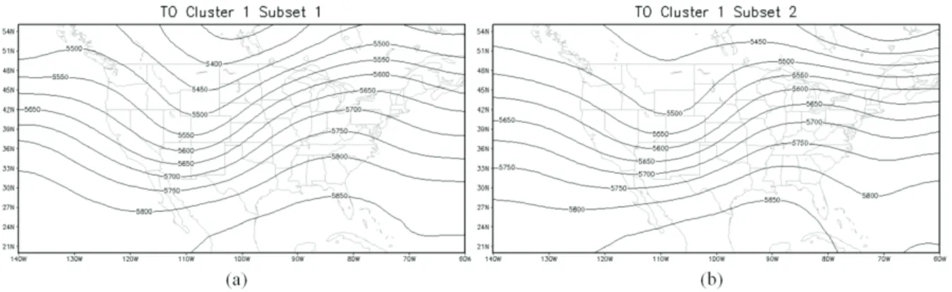
(4) To examine to generalization of our results, the cross-validation was conducted by dividing the training cases into two equal sets by random selection and computing the root mean square error (RMSE) values and correlation between the composites from each subset. Small RMSE values between the two subsets are an indication of good generalization. Many combinations of kernel functions and variables provided excellent generalization (low RMSE) along with high correlation (r≥ 0.95). Maximization of the silhouette coefficient and separation to cohesion ratios were used to identify the optimal number of KPCs and clusters to formulate. These experiments found that the Gaussian radial basis kernel function with σ = 200 optimized silhouette coefficients and separation to cohesion ratios of 0.65 and 4.14 for TOs, respectively, when retaining 1 KPC (variance explained of 14%) and 8 clusters from that KPC. For PNTOs, the silhouette coefficient was 0.64 and the separation-cohesion ratio was 3.48 with 1 KPC (variance explained of 19%) and 7 clusters. The RMSE for 500 mb geopotential height between the TO KPCA subsets was 49.9 m (approx. 0.9% of the average magnitudes of 500 mb geopotential height) and for the PNTOs the RMSE was 48 m (approx. 0.8%). This combination had good generalization as well (e.g. Fig. 1).
Fig. 1. Cluster 1 (RMSE=49.9 m) TO 500 mb geopotential height from KPCA cross-validation using the Gaussian radial basis kernel function with σ=200. Subsets 1 and 2 represent the two halves of the TO data used in the cross-validation.
Once the optimal kernel functions and numbers of clusters were determined for the two outbreak datasets, the composite analyses from the valid time of the event (0000 UTC on the severe weather outbreak day) to 72 hours prior to the outbreak event, at 6 hour intervals, were formulated, leading to 13 3-D atmospheric composites for TOs and PNTOs for each cluster and each compositing method. All composites are centered on the subjective centroid of the severe weather outbreak occurrence, based on storm reports from the Storm Prediction Center. This outbreak-centeredness is critical to ensure that no spatial phase-shift errors occur when grouping or compositing the events. This constraint also signifies that specific geographical locations on the composite charts are arbitrary.
To test the utility of these composites at classifying outbreak type, 40 NTOs and 40 TOs were retained as training data, with the remaining 20 withheld for testing. An SVM classification model was formulated on the TO and PNTO clusters for each method to learn and predict each type of outbreak. The 20 testing outbreaks were used as input into the SVM classification scheme to determine objectively the outbreak type. Since the true outbreak type was known, the results were assessed using traditional contingency statistics (Wilks 2006). This SVM approach is adaptive, since additional cases added to the KPCA or PCA CA will result in modified or new clusters, and training the SVM on these new patterns will result in new types of outbreaks the method can discriminate.
3.Results
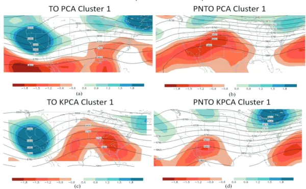
Upon completion of the PCA and KPCA composites, differences in the meteorological data were noted between the two outbreak types. The TO type is associated with a deeper geopotential height trough with positive vorticity values at 500 mb (blue areas in Fig. 2). Both PNTO composites have an upper-level height ridge over the center of the domain, associate with anticyclonic vorticity (red areas in Fig. 2). This type of synoptic weather pattern is most common in summer (evident from analyzing the dates of the 50 associated cases). Two of the 7 PCA-derived PNTO composites and 6 KPCA-derived PNTO composites have a springtime appearance (lower height magnitudes and vorticity centers shifted farther south -- not shown). While at this time it is not evident which composite set is more representative of its constituent members, clear differences exist primarily in the vorticity maxima and minima for the two different compositing methods (congruence coefficients for the normalized height data were 0.99 and for the normalized vorticity data were 0.91 for TOs and 0.6 for PNTOs).
Fig. 2. 500 mb geopotential height (contours, units in m), and vorticity (shaded, units in 10-5 s-1) for the KPCA TO and PNTO
first cluster and the PCA TO and PNTO first cluster. The plots are valid 24 hours prior to the outbreak valid time.
The SVM classification contingency statistics (Table 1) demonstrate that the composites had a perfect probability of detection for TOs (POD = 1) in the independent testing set, though the SVM misclassified 2-3 PNTOs as seen in the false alarm ratio (FAR = 0 would be perfect) showing some misclassification that is was slightly higher with the KPCA composites. Uncertainty arising from sample size and case selection suggests that the results between the two methods were statistically indistinguishable. The skill of the forecast (HSS = 1 would be perfect) did not degrade significantly to lead times of 72 hours, suggesting a strong discrimination capability of the synoptic composites using both methods, though the PCA HSS values were slightly higher.
Table 1. Contingency statistics for the PCA and KPCA SVM classifications of the 20 independent testing outbreak cases. POD values of 1 indicate perfect classification, and FAR values of 0 indicate no false alarms. A HSS value of 1 is perfect skill.
PCA KPCA
Lead Time (h) POD FAR HSS POD FAR HSS
0 1 0.09 0.9 1 0.17 0.8
24 1 0.17 0.8 1 0.23 0.7
48 1 0.17 0.8 1 0.23 0.7
4.Conclusions and Future Work
Synoptic weather composites of TOs and PNTOs were formulated using cluster analysis based on the PCA and KPCA techniques. The goal of the research was to obtain synoptic patterns that discriminate TOs from PNTOs with a high probability of detection, a low false alarm ratio, and to determine the viability of KPCA for representing TO and PNTO composites. The composite maps have some notable differences (Fig. 1), but the contingency statistics (Table 1) from the SVM formulations suggest that PCA and KPCA are virtually indistinguishable for the 100 cases selected. The SVM was successful at discrimination and classification of the two outbreak types, a goal of the work. As additional cases are added to the KPCA or PCA clusters, new and/or revised clusters will emerge, and the SVM will adapt to these changes to distinguish for outbreak type. In future work, the technique will be applied to the entire outbreak period of record from 1979 – present (over 6500 cases), separating events, not only based on their tornadic potential but also based on their overall severity.
Acknowledgements: This work was funded by NSF Grant AGS0831359.
5. References
Barnes, S. L., 1964: A technique for maximizing details in numerical weather map analysis. J. Appl. Meteor., 3, 396–409.
Bell Laboratories, 2011: R version 2.13.0. Mississippi State University
Cristianini, N., and J. Shawe-Taylor, 2000: An Introduction to Support Vector Machines and other Kernel-Based Learning Methods. Cambridge University Press, Cambridge, England, 189 pp.
Doswell, C. A., R. Edwards, R. L. Thompson, J. A. Hart, and K. C. Crosbie, 2006. A simple and flexible method for ranking severe weather events. Wea. Forecasting, 21, 939-951.
Gong, X., and M. B. Richman, 1995: On the application of cluster analysis to growing season precipitation data in North America east Rockies. J. Climate, 8, 897-931.
Kalnay, E., M. Kanamitsu, R. Kistler, W. Collins, D. Deaven, L. Gandin, M. Iredell, S. Saha, G. White, J. Woolen, Y. Zhu, A. Leetmaa, B. Reynolds, M. Chelliah, W. Ebisuzaki, W. Higgins, J. Janowiak, K. C. Mo, C. Ropelewski, J. Wang, R. Jenne, and D. Joseph, 1996. The NCEP/NCAR 40-Year Reanalysis Project. Bull. Amer. Meteor. Soc., 77, 437-471.
Mercer, A., C. M. Shafer, C. A. Doswell III, L. M. Leslie, and M. B. Richman, 2009: Objective classification of tornadic and nontornadic severe weather outbreaks. Mon. Wea. Rev., 137, 4355-4368.
Richman, M. B., and P. J. Lamb, 1985: Climatic pattern analysis of 3 and 7 day summer rainfall in the central United States: Some methodological considerations and a regionalization. J. Clim. Appl. Meteor., 24, 1325 –
1343.
, 1986: Rotation of principal components. J. Climatology, 6, 293-335.
, and I. Adrianto, 2010: Classification and regionalization through kernel principal component analysis.
Phys. And Chem. of the Earth, 35, 316-328.
Roebber, P., D. Schultz, and R. Romero, 2002: Synoptic regulation of the 3 May 1999 tornado outbreak. Wea. Forecasting, 17, 399-429.
Rousseeuw, P.J., 1987. Silhouettes: a graphical aid to the interpretation and validation of cluster analysis. J. Computational and Appl. Mathematics20, 53–65.
Schaefer, J., and C.A. Doswell III, 1984: Empirical orthogonal function expansion applied to progressive tornado outbreaks. J. Meteor. Soc. Japan, 62, 929-936.
Schölkopf, B., Smola, A.J., Müller, K.-R., 1998. Nonlinear component analysis as a kernel eigenvalue problem.
Neural Computation, 10, 1299-1319.
Shafer, C. M., A. E. Mercer, C. A. Doswell, M. B. Richman, and L. M. Leslie, 2009: Evaluation of WRF forecasts of tornadic and nontornadic severe weather outbreaks when initialized with synoptic scale input. Mon. Wea. Rev.,
137. 250-1271.
Swinbank, R., and R. J. Purser, 2006. Fibonacci grids: A novel approach to global modeling. Q. J. R. Meteor. Soc.,
132, 1769 - 1793.