Eustace M. Dogo1, Nnamdi I. Nwulu2, Bhekisipho Twala3, Clinton Aigbavboa4 1,2Dept. of Electrical and Electronic Engineering Science
1Institute for Intelligent Systems
4Dept. of Construction Management and Quantity Survey
Faculty of Engineering and the Built Environment, University of Johannesburg, South Africa 3School of Engineering, Department of Electrical and Mining Engineering, University of South Africa
[email protected], [email protected], [email protected]
Corresponding Author: Eustace M. Dogo, [email protected], Phone: +27 (0) 11 559-2153
Abstract. Traditional machine learning (ML) techniques such as support vector machine, logistic regression, and artificial neural network have been applied most frequently in water quality anomaly detection tasks. This paper presents a review of progress and advances made in detecting anomalies in water quality data using ML techniques. The review encompasses both traditional ML and deep learning (DL) approaches. Our findings indicate that: 1) Generally, DL approaches outperform traditional ML techniques in terms of feature learning accuracy and fewer false positive rates. However, is difficult to make a fair comparison between studies because of different datasets, models and parameters employed. 2) We notice that despite advances made and the advantages of the extreme learning machine (ELM), application of ELM is sparsely exploited in this domain. This study also proposes a hybrid DL-ELM framework as a possible solution that could be investigated further and used to detect anomalies in water quality data.
Keywords: Machine learning, anomaly detection, deep learning, extreme learning machine, smart water grids, water quality
1
Introduction
Water is essential in sustaining life hence it is critical to ensure that water is always safe for drinking and for other uses. It has been well established by experts that many diseases are water-related in nature and these are classified into four categories: waterborne, water-based, water-related, and water-scarce diseases (NHMRC 2011; Waterwise Rand water 2017). Therefore, access to and availability of good quality water leads to improved domestic hygiene and sanitation which experts in the medical field believe improves public health and is critical for national security (Zheling Yang et al. 2014, 2663-2668). Water quality has a significant impact on life expectancy, the burden on health care facilities and the economies of nations. (Sensus 2012) )reported, based on a survey of 182 global water utilities that, around $184 billion is spent annually by utilities on clean water supply, but that a potential annual cost saving of about $12.5 billion could be effected through the implementation of smart water solutions. Potential saving by water utilities globally could thus be huge.
A smart water solution is an integrated approach that enables the automation of processes associated with the operation of a water distribution system (WDS) and routine maintenance of infrastructure (Sensus 2012). It sometimes involves the generation of a large amount of raw data, which can be transformed into useful information leveraging on artificial intelligence (AI) (Sensus 2012; Dogo et al. 2019). A WDS involves facilities or infrastructure used for the collection, treatment, storage and distribution of water from source to consumers, while maintaining the right quality, quantity and pressure (Sensus 2012). The report in (Sensus 2012) also reveals that 41% of surveyed water utilities still rely on manual collection of water samples for analysis, with only 16% relying on automated sampling. Whereas, 40% of these utilities would like to have a real-time water quality monitoring (WQM) system, only 17% currently have one. The remaining 43% of utilities still rely on the manual method of sample collection. In 2015, the United Nations (UN) General Assembly, comprising 193 countries, developed and adopted a proposal on Sustainable Development Goals (SGDs), consisting of 17 goals with 169 targets. SGD goal 6 (SGD 6) is one of the 17 SGDs that call for safe, clean water and sanitation for the entire globe by the year 2030. Safe drinking water is key to protecting citizens from water-related diseases, thus making societies healthier and economically more productive.
It is the opinion of the authors that AI andinformation and communication technology have the potential to synergize the efforts of researchers and all stakeholders in the water industry towards achieving the SDG 6 water target (UN 2015). Continual real-time datasets generated by sensors are key to detecting and understanding
unexpected anomalous and gradual changes in the physical, chemical and biological qualities of water. Several factors are responsible for these changes in water quality. These include the concentration of microscopic pathogens such as bacteria and viruses, quantities of pesticides, insecticides, heavy metals and several other contaminants, as measured by sensors installed in the WDS. These factors are induced or caused by natural disasters such as earthquakes, terrorist attacks and contaminants caused by man-made activities, such as industrial waste (Muharemi, Logofătu, and Leon 2019, 1-14). The raw data collected from these sensors can provide valuable information in support of utilities to enable them to make better decisions, in conjunction with ML techniques, so that proactive and corrective action can be taken in case of contamination to remedy the situation (Zhao, Hou, Huang, and Zhang, 2014). Currently, the concept of smart cities is fast becoming a reality around the world. Smart water networks are an integral part of the smart cities concept that consists of numerous types of private and public connected and interdependent infrastructures, leveraging on internet of things (IoT) and cloud computing technologies, with the overall objective of improving the quality of life of people living in those cities, through improved productivity and efficiency and satisfying customers’ expectations (Garcia-Font, Garrigues, and Rif-Pous 2016, 868; Sensus 2012).
In recent times, there has been increased interest in detecting anomalies in diverse fields, including anomaly detectionand cyber-physical attacks in the WDS (Muharemi, Logofătu, and Leon 2019, 1-14; Shalyga, Filonov, and Lavrentyev 2018; Taormina et al. 2018, 4018048), to enable accurate, faster and better decision support mechanisms (IBM 2017), as a component of an early warning system (Bartrand, Grayman, and Haxton 2017, 1-118). New and innovative technologies are used, with advanced analytics techniques such as ML (Zahra Zohrevand et al. 2016, 1551; Geoffrey E. Hinton, Simon Osindero, and Yee-Whye Teh 2006, 1527-1554; Goodfellow, Bengio, and Courville 2016; Adu-Manu et al. 2017, 1-41; G. Huang et al. 2015, 32-48), largely because of the complexities associated with modern data, such as non-linearity, high dimensionality and the dynamic behaviour of data generated. Of particular interest is the importance of quick response times and high accuracy of detecting contaminants. This is premised on numerous incidents of water contamination that occur yearly worldwide, such as the introduction of cyanide compound into water pipes near a United States (US) embassy in Italy, a direct terrorist attack on US water supply systems (R. Murray et al. 2010, 1-92); water contamination in Japan, the presence of Aeromonas species in a public drinking water supply in Scotland and in tap water in Turkey (Zulkifli, Rahim, and Lau 2017, 2657-2689). Numerous unreported cases occur around the world, especially in developing countries.
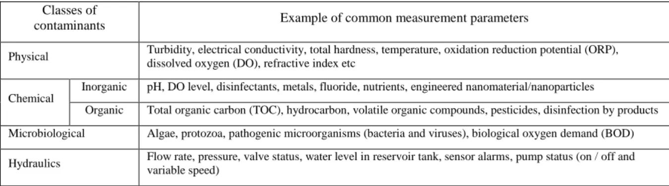
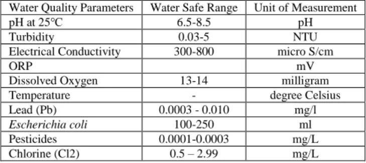
A list of common water quality contaminants and hydraulic parameters in WDSs is summarised in Table 1. Changes in hydraulic parameters, such a flow rate and pressure, are an indication of pipe leakage or burst pipes (Y. Wu and Liu 2017, 972-983), which could result in deterioration of water quality owing to a high possibility of chemical and microbiological contaminants getting into the WDS, thereby triggering anomalies in the water quality dataset. Table 2 shows the World Health Organisation safe drinking water limits of some water quality parameters, which is a compliance guide for water utilities in providing safe drinking water for citizens.
Table 1. Common water quality contaminants and hydraulic parameters Classes of
contaminants Example of common measurement parameters
Physical Turbidity, electrical conductivity, total hardness, temperature, oxidation reduction potential (ORP), dissolved oxygen (DO), refractive index etc
Chemical
Inorganic pH, DO level, disinfectants, metals, fluoride, nutrients, engineered nanomaterial/nanoparticles
Organic Total organic carbon (TOC), hydrocarbon, volatile organic compounds, pesticides, disinfection by products Microbiological Algae, protozoa, pathogenic microorganisms (bacteria and viruses), biological oxygen demand (BOD) Hydraulics Flow rate, pressure, valve status, water level in reservoir tank, sensor alarms, pump status (on / off and variable speed)
Table 2. World Health Organisation Limits of Safe Drinking Water Water Quality Parameters Water Safe Range Unit of Measurement
pH at 25℃ 6.5-8.5 pH
Turbidity 0.03-5 NTU
Electrical Conductivity 300-800 micro S/cm
ORP mV
Dissolved Oxygen 13-14 milligram
Temperature - degree Celsius
Lead (Pb) 0.0003 - 0.010 mg/l
Escherichia coli 100-250 ml
Pesticides 0.0001-0.0003 mg/L Chlorine (Cl2) 0.5 – 2.99 mg/L
This survey paper focuses on review of water quality anomaly detection (WQAD) using AI approaches, more specifically ML methods for water quality anomaly detection across several academic databases particularly in the ScienceDirect, IEEE Xplore and Google Scholar databases. Publications between 2002 and 2018 were considered, since the intensification of research on water quality anomaly detection occurred after the 11 September 2001 attacks. The general search query use is “Water Quality Anomaly Detection” AND “Artificial Intelligence” OR “Machine Learning” AND “Water Distribution System”. Additional query modifications were filtered based on ML: Traditional ML including extreme learning machine (ELM) and deep learning (DL) techniques. For each paper identified, the following attributes were used for reporting: study domain, dataset used, data parameter investigated, method applied, performance metrics and findings.
This study reviews DL frameworks in addition to most used traditional ML methods that are used for WQAD in WDSs. Hybrid frameworks could be exploited to address some of the challenges associated with the traditional and supervised anomaly detection methods identified earlier.It will hence be interesting to see how they would perform in this task to achieve better results in comparison to already existing studies.
The contribution of this survey study is:
1. To carry out a systematic literature review in order to ascertain the current ML techniques used for the WQAD problem.
2. To highlight the shortcomings and limitations of these current methods
3. To propose a hybrid DL-ELM framework in WQAD, which could be investigated further 4. To recommend future research directions
2.
Background and Literature Review
Anomaly detection is a process of discovering patterns in a dataset that do not conform to expected notions of normal behaviour or fit well in a dataset (Chandola, Banerjee, and Kumar 2009). In the context of this paper, anomaly seeks to detect unusual or suspicious observations caused by either intentional or unintentional attacks, or failure in one of the system's components or events of interest in the WDS. For example, unusual chlorine content in water will indicate low water quality, whereas, changes in flow rate and pressure will indicate a leak, which could comprise the water quality in the pipelines. Anomaly detection is often used interchangeably with
outlier detection, novelty detection, noise detection, deviation detection or exception mining (Hodge and Austin 2004, 85-126) or as a surprise in cognitive science (C. Wu and Guo 2015, 181-186; Ahmed, Mahmood, and Hu 2016, 19-31). Surprise is defined as the divergence between a sensing target’s internal approximation with the model and the real environment, based on free-energy principles (Friston 2009, 293-301). The choice of term is mainly based on the authors’ preferences and perspectives, but the definitions and techniques employed in detecting these terms are fundamentally similar (Hodge and Austin 2004, 85-126).
Anomaly detection algorithms could be broadly sub-divided into four main categories:statistical, classification, information theory and clustering based algorithms (Pimentel et al. 2014, 215-249; Ahmed, Naser Mahmood, and Hu 2016, 19-31). Anomaly detection usually attempts to quantify normal or abnormal behaviour flagging irregular behaviour as possibly anomalous (Yolacan and Kaeli 2016, 39-50). The challenges of anomaly detection are defining what constitutes normal for a given subject area, deciding what degree of the observed activity to flag as abnormal, and how to make that decision (Axelsson 1998). A significant amount of survey on anomaly detection has been carried out across numerous domains (Hodge and Austin 2004, 85-126; Chandola, Banerjee, and Kumar
2009; Pimentel et al. 2014, 215-249; Patcha and Park 2007, 3448-3470; Ahmed, Naser Mahmood, and Hu 2016, 19-31) and research has been done in many application areas: aviation (Das et al. 2013, 2668-2673; Janakiraman and Nielsen 2016, 1993-2000), network infrastructure in smart cities (Difallah, Cudré-Mauroux, and McKenna 2013, 39-47), water quality and smart cities (D. Zhang et al. 2014; Abid, Kachouri, and Mahfoudhi 2017, 1-4), electric power systems (Martinelli et al. 2004, 1242-1248), earthquake studies (Akhoondzadeh 2015, 1200-1211), transfer representation learning (Andrews et al. 2016), web layer cloud (Kozik et al. 2017, 226-233) and computational biology (Görnitz, Braun, and Kloft 2015, 1833–1842).
The following are well-known challenges associated with anomaly detection research (Ahmed, Mahmood, and Hu 2016, 19-31; Erfani et al. 2016, 121-134):
Since anomalies are rare to find in most cases, there is the issue of imbalance in the anomalous-to-normal data ratio, which could affect the accuracy of a prediction model by exhibiting high false positive rates. A high false positive rate measures the proportion of non-anomalous events or behaviour that is wrongly classified as anomalous: it is equivalent to a false alarm.
Lack of a universally accepted anomaly detection technique that could be applied across domains is problematic. It then becomes a challenge to researchers to find methods that would be most suitable for any given problem and domain. For example, an anomaly detection technique in internet activities with a labelled dataset or in financial transactions may not be useful for WQAD in WDS with the unlabelled dataset.
Difficulty in differentiating noise, missing data, inaccurate or faulty sensors reading with an anomaly in the dataset
Ii is difficulty with obtain publicly available and real-world datasets from utilities to be used for testing and evaluating WQAD models owing to privacy and legal concerns.
Increased false alarms are generated by ML models owing to training with a limited dataset.
Account must be taken of dynamic behaviour of anomalies in time series and continual evolving of normal, as what is termed normal today maybe abnormal tomorrow and vice versa. For example, 1) an increase in population and water usage pattern by consumers can change over time; 2) anomaly detection techniques may become obsolete with time owing to the complex nature of data and attack scenarios on the WDS.
2.1 Types of Anomalies
There are three main types of anomalies (Chandola, Banerjee, and Kumar 2009), which are briefly discussed: Point anomaly: This occurs when a single data instance, is detached from the normal pattern in the rest of the
dataset. For example, if a normal household’s water consumption is 1500 litres per day and it suddenly becomes 3000 litres on any given day, it is a point anomaly.
Contextual anomaly: These are data instances that are considered as anomalies in a specific context only. For example, during
a
heat wave in summer, water consumption is usually higher than during the rest of the year. Although higher, it may not be termed anomalous but contextually normal. Contextual anomaly is also referred to as conditional anomaly. Collective anomaly: When a collection of similar data instances behaves anomalously with respect to the entire dataset, the group of data instances is termed a collective anomaly. Single data instances in a collective anomaly will possibly not be considered anomalies by themselves, but the collection of single data instances together could indicate a collective anomaly.
Factors such as the nature of the dataset, availability of labelled data, type and nature of anomalies to be detected and application domain often determine the anomaly detection technique to be employed (Ahmed, Mahmood, and Hu 2016, 19-31).
3.
Water Quality Anomaly Detection Studies
Water quality is terminology that describes the physical, chemical, and biological features of water, in relation to its suitability for an intended purpose or use(South African 2017). The key aspect is ensuring that the quality of water is suitable for its intended use in line with approved standards. Hence, the overall objective of water quality anomaly is to detect contamination more quickly and accurately.
3.1 Traditional Manual Water Quality Monitoring Approach
WQM for anomaly detection over the years has evolved from a traditional manual laboratory-based approach to traditional manual in situ methods (Adu-Manu et al. 2017, 1-41). More recently techniques based on wireless
sensor networks (WSN) have been used, where real-time sensor measurements are analysed using data analytic methods to detect abnormal events. The common traditional WQM methods are briefly discussed as follows:
Physical Observation: Water quality is usually judged through observation of contaminants in the water. This to an extent is still prevalent today, with water utility personnel and consumers still acting as sensors and offering insights into the safety of drinking water based on the observed presence or absence of specific water quality indicators.
Laboratory-based Analysis Method: This method is still very much in use by water utility companies, where water samples are taken randomly or at specified time intervals for laboratory analysis by highly skilled personnel, using specialised equipment to ascertain the safety of drinking water. Several laboratory-based methods exist, which vary in terms of contaminant to be detected, sensitivity, and time taken for detection. However, these methods can only account for the time and place the sample is taken, and not the entire WDS.
Handheld Detection Devices: Handheld portable devices sometimes with wireless network capabilities, have been developed and are currently used for water contaminant detection in small water bodies.
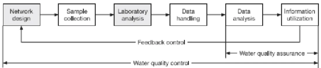
A general traditional WQM framework is shown in Fig 1, which involves several stages from network design to information utilisation.
Fig. 1. Traditional WQM framework (Adu-Manu et al. 2017, 1-41)
Drawbacks: These traditional WQM methods are time-consuming and challenging in detecting contaminants in low concentrations. Moreover, they cannot meet the needs of real-time, multiple and heterogeneous water quality parameters, as well as the need for high accuracy detection of water quality events across the entire WDS, hence the need for detection using AI techniques on data obtained from stationed on-site multiple water quality sensors.
3.2 Wireless Sensor Networks Approach
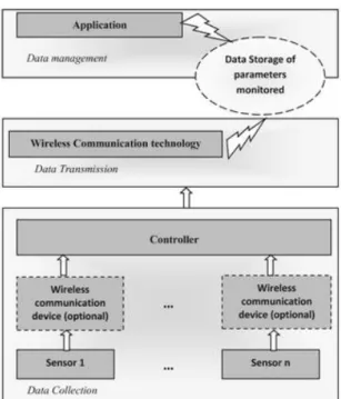
Advances in WSNs are key to their adoption for water quality analysis for anomaly detection as opposed to the traditional manual methods because of the aforementioned challenges. A detailed survey on WSN and its application in numerous environmental monitoring domains which are also applicable to the smart water grid, are provided by (Akyildiz et al. 2002, 393–422). Of the five common smart grid systems: electricity, gas, telecommunication, transportation and water, the smart water grid remains underdeveloped despite tremendous progress in sensor technology and data analytics. This may partly be attributed to slower progress by water utility companies embracing new technologies. However, despite the perceived slow rate of adoption of these technologies by the water utilities, progress has been mad recently in the deployment of interconnected sensor devices that allow for continuous collection and analysis of data in real-time. Data analytics capable of extracting useful information from the massive amount of data generated by these real-time sensor devices for large-scale WDS remains a major challenge in the research and academic ecosystem (Difallah, Cudré-Mauroux, and McKenna 2013, 39-47). A general smart water monitoring framework is depicted in Fig. 2, comprised of three layers. The first is the collection of water quality parameters data by wireless sensors, which are sent to a controller. The next is data transmission using suitable wireless communication technology, depending on the distance of communication, followed by data management where data analysis is carried out (Geetha and Gouthami 2017, 1-19)
Fig. 2. Wireless Communication technology Data Transmission (Geetha and Gouthami 2017, 1-19)
Real-time sensor readings are usually captured over the course of time, referred to as time-series measurements (Gamboa 2017), which makes the dataset challenging to analyse with traditional ML techniques. A time-series is defined (Gamboa 2017) as a vector 𝑋 = {𝑥(1), 𝑥(2), ⋯ , 𝑥(𝑛)}, where each element 𝑥(𝑡)∈ 𝑅𝑚 relating to 𝑋 is an array of 𝑚 values such that {𝑥1(𝑡), 𝑥2(𝑡), ⋯ , 𝑥𝑚
(𝑡)
}. Each one of the 𝑚 values corresponds to the input variables measured in the time-series. The rate at which data are measured in time-series is called the sampling frequency. The sampling frequency gives the granularity of the data sampling, which is the average number of samples per given time.
A water quality contamination warning system is an integrated system that enables monitoring and detection of contamination events and provides timely alert warnings using advanced technologies for data analysis. This system consists of an online monitoring system, supervisory control and data acquisition (SCADA), event detection system, and decision support system (Zhao et al. 2014, 1-15). The US Environmental Protection Agency (USEPA) and Sandia National Laboratories are the main research organisations that focus on real-time water anomaly event detection algorithms based on time-series with a linear filter or autoregressive moving average, k-mean clustering and binomial event discriminator. The algorithms are integrated to form an event classification model in an open source software called CANARY. However, the growing amount of real-time heterogeneous data these wireless sensing devices are expected to generate, taking into account the notion of time, motivates researchers to explore newer data analytic methods such DL, hybrid or ensemble approaches for the emerging big sensor data concept and trend (L. Chen and Kang 2015, 1020-1026; Y. Zhang et al. 2016, 155-166), with the purpose of achieving better results, as opposed to the traditional ML approaches that do not adequately handle these data instances.
Over the past decade academic scholars and research organisations such as the USEPA, Harvard University Water Security Initiative, and Abdul Latif Jameel Water and Food Systems Lab in the Massachusetts Institute of Technology (J-WAFS) have spearheaded a tremendous amount of interdisciplinary research on a wide range of domains, including securing the WDSs to address vulnerabilities as fallout of the events on 11 September, 2001, to detect and respond to possible accidental and intentional attacks, as well as modernising water utilities for enhanced efficiency informed by science and technological advancements. The science and engineering research focus could be broadly categorised as shown in Table 3 (Bakker et al. Nov 4, 2012):
Table 3. Summary of Science and Engineering Research Direction Related to WQAD
S/N Research Focus Study
1 Sensor development for detection of contaminants
(Hall 2009; Raich 2013, 1-33; Tatari et al. 2016; Zulkifli, Rahim, and Lau 2017, 2657-2689)
2 Optimal sensor placement for contamination and leak detection in WDS
(Eliades, Kyriakou, and Polycarpou 2014, 602-611; Mukherjee, Diwekar, and Vaseasht 2017, 91-102; Propato, Cheung, and Piller 2006, 1-8; Rathi and Gupta 2014, 181-188; Rosich, Sarrate, and Nejjari 2012, 776-781; Casillas et al. 2013, 14984-15005; Berry et al. 2006, 218-224; R. Murray et al. 2010, 1-92)
3 Real-time monitoring via WSN
(Allen, Preis, and Iqbal 2013; Lambrou et al. 2014, 2765-2772; Zabasta et al. Sept 2014, 42-47)
4 Identification of the source of contaminants
(Deuerlein, Meyer-Harries, and Guth 2017, 53-59; Propato, Cheung, and Piller 2006, 1-8; Klise et al. 2016, 4016001)
5 Optimal response after detection of contaminants to mitigate adverse effects on public health
(Mukherjee, Diwekar, and Vaseasht 2017, 91-102; Rasekh and Brumbelow 2014, 12–25)
6 Anomaly detection using AI and data mining techniques
Deng and Wang, 2017; Inoue, Yamagata, Chen, Poskitt, and Sun, 2017; Tian, Jiang, Guo, and Wang 2012; Vries, van den Akker, Vonk, de Jong, and van Summeren, 2016; Zohrevand et al. 2016; Zhang et al. 2014; Zhang, Zhu, Yue, and Wong 2017.
According to (Raciti, Cucurull, and Nadjm-Tehrani 2012, 98-119), water quality anomaly detection in WDS can be categorised into two namely, hydraulic fault anomaly, which deals with mechanical systems, and water quality anomaly, which has to do with anomalous changes of water as a result of accidental or intentional injection of contaminants into the WDS. However, hydraulic fault anomaly such as a change in flow rate or pressure could indicate a pipe burst and contaminants finding their way into the WDS.
4.
Artificial Intelligence Methods
4.1 Overview of Traditional Machine Learning Methods
Support vector machine (SVM), logistic regression (LR), linear discriminant analysis (LDA), and artificial neural networks (ANN) are the traditional (ML) methods that have gained most attention in recently time in WQM and anomaly detection (F. Muharemi et al. 2018, 173-183). Aside from these traditional ML methods, statistical methods are also trusted for anomaly detection of water quality data. Multivariate techniques such as principal component analysis and linear discriminant analysis have also been applied in this area of study (F. Muharemi et al. 2018, 173-183). Because of space constraints, the theoretical background of these traditional ML techniques is not covered however, readers are referred to (F. Muharemi et al. 2018, 173-183) for details.
Most of these traditional ML techniques suffer drawbacks, as they are associated with high computational memory and time complexities, an imbalanced anomalous-to-normal data ratio and sensor signal processing noise, resulting in high false alarm rates, poor handling of missing data, a low level of accuracy and lack of robustness in handling real-time big datasets from multiple and heterogeneous sensory sources in high dimensional data search space (Ahmed, Naser Mahmood, and Hu 2016, 19-31; Erfani et al. 2016, 121-134; Muharemi, Logofătu, and Leon 2019, 1-14). DL model architectures have consequently lately also started being considered. Therefore, it becomes necessary to investigate other novel anomaly detection techniques to improve performance and overcome the shortcomings of these ML methods. This work is motivated by earlier works that show ML techniques producing good results for WQAD tasks (Muharemi, Logofătu, and Leon 2019, 1-14) and good prospects in using hybrid DL and one-class SVM models for anomaly detection tasks (Erfani et al. 2016, 121-134). A ML technique that is not quite recent but has enjoyed a tremendous research following is ELM. A brief theoretical background is given in the subsequent subsection.
4.2 Extreme Learning Machine
Motivated by the learning speed of feedforward neural networks, which is generally considered much slower than expected owing to slower iterations and parameter tuning of the networks, Huang et al proposed ELM algorithm. The classical ELM consists of a three-layer feedforward architecture. The first layer acts as the input, and the second is the only hidden layer. The connection weights between the input and hidden layers are randomly generated, set and fixed without being altered for the entire duration of the network, the hidden layer then projects the input layer to a higher dimensionality. Using non-linear sigmoid activation functions the outputs from the hidden layer are generated. The third layer acts as the output and has linear input-output characteristics. Using the training data, the connection weights between the hidden and output layers are trained and analytically determined in a single pass using a regularised least square method, such as the Moore-Penrose pseudo-inverse, to calculate the hidden layer values and the desired output (Tissera M.D., McDonnell M D 2015, 325-354). ELM is mathematically described as follows:
For any given N distinct training samples (𝑥𝑖, 𝑡𝑖) ∈ 𝑅𝑛, with 𝑁̃ hidden nodes and activation function is
mathematically represented as,
𝑜𝑗= ∑ 𝛽𝑖𝜎𝑖(𝑥𝑗) = ∑ 𝛽𝑖𝜎(𝑤𝑖∗ 𝑥𝑗+ 𝑏𝑗) 𝑁̃ 𝑖=1 𝑁̃ 𝑖=1 , 𝑗 = 1, … , 𝑁 (1) where 𝑜𝑗 is the output vector of the Single hidden-layer feedforward neural network (SLFN) with regards to the
input sample 𝑥𝑖, and 𝑏𝑗 are learning parameters generated randomly by the jth hidden node, representing the
biases of the hidden layer neurons. 𝛽𝑖= [𝛽𝑖1, 𝛽𝑖2, … 𝛽𝑖𝑚]𝑇is the link connecting the jth hidden node and the output
nodes, which represents output weights, and 𝜎(𝑤𝑖∗ 𝑥𝑗+ 𝑏𝑗) is the activation function. When 𝑤𝑖∗ 𝑥𝑗 is set as an
inner product, equation (1) assumes the following form:
𝑯𝜷 = 𝟎 (2) where, 𝐻 = [ 𝜎(𝑤𝑖∗ 𝑥𝑗+ 𝑏𝑗 ⋯ 𝜎(𝑤𝑁̃∗ 𝑥𝑗+ 𝑏𝑁̃ ⋮ ⋮ ⋮ 𝜎(𝑤𝑖∗ 𝑥𝑁+ 𝑏𝑗) ⋯ 𝜎(𝑤𝑁̃∗ 𝑥𝑁+ 𝑏𝑁̃ ] 𝑁×𝑁̃
𝑯 is the hidden layer output matrix of the neural network.
𝜷 = [ 𝛽1𝑇 ⋮ 𝛽𝑁̃𝑇 ] 𝑁̃×𝑚 , 𝑶 = [ 𝑜1𝑇 ⋮ 𝑜𝑁𝑇 ] 𝑁×𝑚
To minimise the network cost function ‖𝑂 − 𝑇‖, and based on the ELM theories that the hidden nodes 𝑤𝑗 and 𝑏𝑗
learning parameters are randomly assigned without considering the input data. Equation (2) assumes a linear system and the output weights are defined by finding a least-square solution, which is given as:
𝜷̂ = 𝑯†𝑻 (3)
where 𝐻† is the Moore-Penrose generalised pseudo-inverse of the matrix 𝐻 (G. Huang, Zhu, and Siew 2006a,
489-501)
In the case where the training patterns are more than the number of the hidden neurons, which is usual in most cases, a regularised ELM is obtained to improve the generalisation and robustness of the solution for 𝛽̂, which then assumes this form:
𝜷̂ = (𝑰 𝑪+ 𝑯
𝑻𝑯) −𝟏
𝑯𝑻𝑯 (4)
where 𝐼 is called the identity matrix of dimension L and 𝐻𝑇𝐻 is called the ELM kernel matrix for the ELM kernel
ℎ(𝑥𝑖) ∙ ℎ(𝑥𝑗) (G. Huang et al. 2015, 32-48)
As opposed to backpropagation (BP) based neural networks, iterations and parameter tuning are absent in ELM. Fast training and good generalisation which is the ability to perform well on new inputs unseen previously other than those trained by the model, are the main strengths of the ELM algorithm, hence its wide application in ML
research (G. -. Huang, Chen, and Siew 2006, 879-892). Extensive studies conducted by various researchers have aimed at improving the original ELM’s performance in terms of theories and applications.
Despite the popularity of ELM in the research realm, to the best of our knowledge no studies are currently being conducted on WQAD using ELM. However, because of training speed and good generalisation performance, ELM is gaining a lot of attention among researchers in tackling anomaly detection problems in other domains, as reported in studies by (Ding, Xu, and Nie 2014, 549-556; G. Huang, Zhu, and Siew 2006b, 489-501; Janakiraman and Nielsen 2016, 1993-2000; Wang et al. 2015, 415-425). It will be interesting to see how it performs in the drinking-water anomaly detection task.
4.3 Deep Learning
DL is a sub-domain of ANNs, which is a ML algorithm inspired by the structure and function of the human brain. It emulates the concept of several layers of the human neocortex, capable of self-learning data features by imitating the self-learning process layer by layer in the human visual cortex, which processes visual stimuli and creating a data-driven model with the given dataset ((Z. Y. Wu, El-Maghraby, and Pathak 2015, 479-485). DL is a study of learning models with multilayer representations and heavily based on knowledge drawn from statistics, neuroscience and applied mathematics (Goodfellow, Bengio, and Courville 2016). DL scales well for large amount of data, better programming software and advances in fast computer architectures and hardware system designs. DL can also discover and learn good representations in dataset using feature learning. The learning algorithm’s success depends to a large extent, on how well data are represented (Bengio 2009, 1-127; Bengio 2012, 17-37). DL is described as an ANN approach with many layers of depth in the architectural models (Goodfellow, Bengio, and Courville 2016), hence the phrase “deep”. Another recent definition is captured in (LeCun, Bengio, and Hinton 2015, 436) with emphasis on the multi-layered approach of DL. The main DL architectural models are convolutional neural network (CNN) (LeCun et al. 1998, 2278-2324), recurrent neural networks (RNN) (Rumelhart, Hinton, and Williams 1986, 318-362), stacked denoising autoencoder (SDAE) (Vincent et al. 2010, 3371-3408), deep belief network (DBN) (Geoffrey E. Hinton, Simon Osindero, and Yee-Whye Teh 2006, 1527-1554), deep boltzmann machine (DBM) (Salakhutdinov and Hinton 2009, 448-455) and their respective variations.
4.3.1 Deep Learning Architectural Models
Convolutional Neural Network
CNN is the most widely used DL model in the areas of computer vision, image process, speech recognition and natural language processing and in anomaly detection for drinking water using BiLSTM ensemble technique (Chen, Feng, Wu and Liu, 2018). CNN employs a convolutional mathematical operation at the CNN layers to derive a weighting function w(a), where a is the age of measurement for time series data. By applying a weighted average operation at every time interval, the convolution operation is generally defined as follows:
𝑠(𝑡) = ∫ 𝑥(𝑎)𝑤(𝑡 − 𝑎)𝑑𝑎 = 𝑠(𝑡) = (𝑥 ∗ 𝑤)(𝑡) (5) where 𝑥 is input and 𝑤 as the kernel or filter, and 𝑠 the output called the feature map for continuous time series 𝑡. The discrete convolution operation with the assumption that 𝑥 and 𝑤 are defined based on integer values of 𝑡 will assume the following form:
𝑠(𝑡) = (𝑥 ∗ 𝑤)(𝑡) = ∑ 𝑥(𝑎)𝑤(𝑡 − 𝑎)
∞
𝑎=−∞
(6)
CNN differs from the usual neural network layers by having 1) sparse interactions whereby the kernel is made smaller than the input, by using only meaningful features that translate to fewer parameters and operations to compute the output with better model statistical efficiency, 2) parameter sharing, which refers to the use of one weight value or parameter for multiple functions in a model, and 3) equivariant representation, where output changes when input changes in the same manner (Goodfellow, Bengio, and Courville 2016). Significant research progress has been made in detecting microbiological parasites and bacteria through images obtained from sensors to assess water quality in real-time data such as, E-coli sense sensor (Ecoli Sense 2019). Labelled images obtained
from these sensors could be fed into a CNN model for classification of water as bacteria infected or not infected. This will possibly give an indication of the water quality.
Recurrent Neural Network and Long Short-Term Memory
RNN (Graves 2013) is a feedforward neural networks model with feedback loops that recursively processes each variable-length sequence input values 𝑥 = (𝑥1, … 𝑥𝜏) while maintaining its internal hidden state h. This means
that the output of the RNN model is a function of not only the current input, but also of the previous output. RNN is trained with BP. Generally, RNN comprises three layers, namely input, recurrent hidden and output. RNN has N sequential input values 𝑥𝑡𝑖 and sequential 𝑦𝑡𝑖 through time stamp from t to 𝜏. The hidden layer has M hidden
ℎ𝑡𝑖values. However, because of the challenge of learning long-term dependencies in sequential data, storing
information for a very long time becomes very hard, which makes RNN suffers a set-back in vanishing gradient descent during BP. Long short-term memory (LSTM) addresses this weakness in RNN by providing longer-term memory and non-linear gating units to control how information enters and leaves the gated cells. Deeper treatment of LSTM variants is provided in (Greff et al. 2017, 2222-2232).
Autoencoder
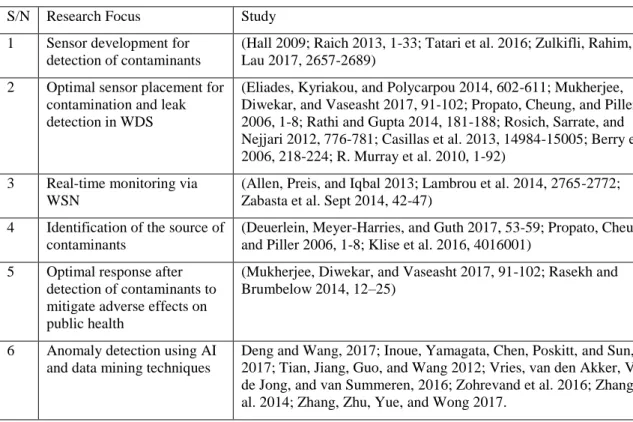
Autoencoder (AE) is an unsupervised neural network learning algorithm using BP, where the target values are set to be equal to the input values as 𝑦𝑖= 𝑥𝑖 (Goodfellow, Bengio, and Courville 2016). The architecture of the AE
learning algorithm is shown in Fig. 3 (Andrew Ng 2011, 72).
Fig. 3. Architecture of autoencoder learning algorithm (Andrew Ng 2011, 72)
Comprising three layers, input, hidden and output layers, the AE tries to learn to approximate the function ℎ𝑊,𝑏(𝑥) ≈ 𝑥, to output 𝑥̂ that is like 𝑥. The AE network has two main parts: an encoder function ℎ = 𝑓(𝑥) which
transforms the input data to a low-dimensional code and a decoder that reconstructs the data from the code 𝑥̂ = 𝑔(ℎ) = 𝑔(𝑓(𝑥)). Hence AE could be mathematically represented as follows:
𝑥̂ = 𝑔(𝑊𝑥 + 𝑏) (7)
where 𝑥 is the input, 𝑊 is the weights, 𝑏 is the bias and 𝑔 is the sigmoid or rectified activation function.
AE is generally good for dimensionality reduction and in unsupervised nonlinear feature extractor problems. AE has numerous enhanced variants such as SDAE and sparse AE (Andrew Ng 2011, 72)
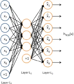
Restricted Boltzmann Machine
A restricted boltzmann machines (RBM) is a deep probabilistic model that is an undirected probabilistic graphical model made up of a layer of visible variables and a single layer of hidden variables connected by symmetrically undirected weights as shown in Fig. 4 (Chu et al. 2017). RBMs could be stacked on one another to produce deeper models (Goodfellow, Bengio, and Courville 2016).
Fig. 4. Restricted boltzmann machine model (Chu et al. 2017)
An RBM is an energy-based model and its joint probability distribution taking into account its energy function, is given as:
𝑃(𝑣, ℎ) =1
𝑍exp(−𝐸(𝑣, ℎ)) (8)
where 𝐸(𝑣, ℎ) is the RBM energy function given by:
𝐸(𝑣, ℎ) = ∑ 𝑎𝑖𝑣𝑖− ∑ 𝑏𝑗ℎ𝑗 𝑗∈ℎ𝑖𝑑𝑑𝑒𝑛 − ∑ 𝑣𝑖ℎ𝑗𝑤𝑖𝑗 𝑖.𝑗 𝑖∈𝑣𝑖𝑠𝑖𝑏𝑙𝑒 (9)
where 𝑣 = (𝑣1, 𝑣2… 𝑣𝑛) 𝑎𝑛𝑑 ℎ = (ℎ1,ℎ2… . ℎ𝑚) are the visible and hidden vectors; 𝑎𝑖 𝑎𝑛𝑑 𝑏𝑗 are their biases;
n and m are the visible and hidden layers dimension and 𝑤𝑖𝑗 the connection weight matrix between the visible
and the hidden layers, while 𝑍 is the normalising constant called the partition function and mathematically defined as the summation of all pairs of visible and hidden layers possible:
𝑍 = ∑ ∑ exp(−𝐸(𝑣, ℎ))
ℎ 𝑣
(10)
Deep Belief Network
A DBN is a hybrid stacked RBM made up of both directed and undirected connections, with multiple hidden layers, usually trained using BP. DBN, unlike RBM, has many hidden layers. RBM normally has only one hidden layer. Figure 5 shows a three-layer configuration with two hidden layers and one visible layer, with the top two-layer connection undirected, but with the other two-layers connected and directed toward the two-layer nearest to the data, but with no intra-layer connections except between units in neighbouring layers (Goodfellow, Bengio, and Courville 2016).
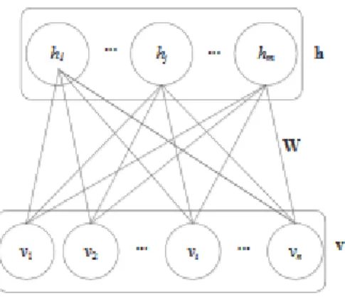
Deep Boltzmann Machine
DBN neural network is an undirected graphical connection model with variables inside all layers and made of several stacked layers and hidden variables, more than in the RBM model. A typical DBM graphical model is shown in Fig. 6 (Goodfellow, Bengio, and Courville 2016), made up of two top hidden layers and one visible bottom layer. In the DBM model, there are no intra-unit layer connections, except between units in neighbouring layers.
Fig. 6. Deep Boltzmann machine graphical model (Goodfellow, Bengio, and Courville 2016)
Several anomaly detection studies using DL exist in literature, showing for example that the application of deep belief network learning algorithm in smart water networks performs better when compared to the traditional ANN (Z. Y. Wu, El-Maghraby, and Pathak 2015, 479-485). Deep structured energy-based models, adopt energy score and reconstruction error as decision criteria for anomaly detection (Zhai et al. 2016). Autoencoder is also proposed in the domain of WDS (Taormina and Galelli 2018, 4018065; Chandy et al. 2019, 4018093).
5.
Machine Learning Techniques and Data used in WQAD
Table 4 shows a comparison of different ML models based on the F-score of the GECCO challenge public water company Thüringer Fernwasserversorgung dataset
(SPOTSeven Lab 2017)
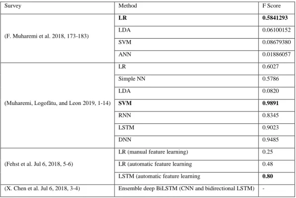
. The result in (F. Muharemi et al. 2018, 173-183) shows the linear regression statistical model achieving a better F-score compared to the other evaluated ML models. The use of only two parameters rather than using all input parameters played a significant part in the result obtained. The authors acknowledge that SVM and ANN could achieve results if all parameters are used with enough training time on the models.In an extended work, (Muharemi, Logofătu, and Leon 2019, 1-14) went further to evaluate the performance of ML when compared to LR model. According to the result obtained, SVM showed better performance on a time series-based dataset in comparison to LR, even though generally the other evaluated ML models also did well. However, the authors observed that SVM, ANN and LR were less susceptible to an imbalanced dataset, while the DNN, RNN and LSTM DL models were more susceptible to it.
The effect of automatic feature learning, when compared to manual feature learning on drinking-water quality anomaly detection using ML models, is further observed (Fehst et al. Jul 6, 2018, 5-6). LSTM with automatic feature learning showed superior performance with an F-score of 80% when compared to the statistical LR model with an F-score of 48%.
The work by (X. Chen et al. Jul 6, 2018, 3-4) using an ensemble CNN and bidirectional LSTM (deep BiLSTM) model claims suitability of the proposed framework for the drinking-water quality anomaly detection dataset, in terms of handling time series and the imbalanced data problem, although no performance metric value was given in the study.
The overall conclusion is that ML models are generally suitable for drinking-water quality anomaly detection problems if time series and imbalanced dataset problem are well captured in the architectural model implementation. This forms a basis for justification and motivation for researchers to explore other ML architectural frameworks/models that could possibly improve the performance of WQAD problems.Table A. 6 presents a summarised performance of traditional and deep ML techniques applied to WQAD.
Table 4. Comparison of some ML Models on GECCO Dataset (SPOTSeven Lab 2017)
Survey Method F Score
(F. Muharemi et al. 2018, 173-183)
LR 0.5841293
LDA 0.06100152
SVM 0.08679380
ANN 0.01886057
(Muharemi, Logofătu, and Leon 2019, 1-14)
LR 0.6027 Simple NN 0.5786 LDA 0.0820 SVM 0.9891 RNN 0.8345 LSTM 0.9023 DNN 0.9485
(Fehst et al. Jul 6, 2018, 5-6)
LR (manual feature learning) 0.25 LR (automatic feature learning 0.48 LSTM (automatic feature learning 0.80
(X. Chen et al. Jul 6, 2018, 3-4) Ensemble deep BiLSTM (CNN and bidirectional LSTM) -
5.1 Performance Metrics for Evaluating WQAD Methods
Performance metrics for comparing experimental results in ML study are fundamental in evaluating the quality of models (Ferri, Hernández-Orallo, and Modroiu 2009, 27-38). The most commonly accepted performance evaluation methods in WQAD classification problems are accuracy, precision, recall and the F-score. However, the authors in (F. Muharemi et al. 2018, 173-183) advocate the use of a combination of these different metrics to assess the goodness of fit for models better, as reliance on only one metric, such as accuracy, may be misleading. We present a brief definition of these commonly used metrics:
Confusion matrix: This is an n x n matrix, where n is the number of classes being predicted. For anomaly detection using a binary classification problem, n=2, we, therefore, will have a 2 x 2 matrix as shown on Table 5.
Table 5. Confusion Matrix for Two-class Scenario Predicted class
Actual class
Class =Anomaly = Yes Class = Not Anomaly= No Class = Anomaly = Yes True Positive (TP) False Negative (FP) Class = Not Anomaly = No False Positive (FP) True Negative (TN)
True Positives (TP): These are the correctly predicted positive class or value. It means that the actual event is anomaly detected is True = Yes and the predicted class is also True = Yes
True Negatives (TN): These are the correctly predicted negative class or value. It means that the actual event, no anomaly detected is False = Yes and the predicted class is also False = Yes.
False Positives (FP): This occurs when the actual class contradicts the predicted one. In this case, it means that the actual event, no anomaly, is False = No and the predicted class is False = Yes
False Negative: This occurs when predicted class contradicts the actual one. In this case, it means that the actual event, anomaly detected, is True = Yes and the predicted class is True = No.
Accuracy: This is the total number of correctly classified predictions, so it means the number of predicted events or observations divided by the total number of events or observations. Accuracy is a very intuitive performance metric and is dependent on whether the dataset is balanced or imbalanced, that is, the ratio of anomalous and non-anomalous events in the data set. However, because in real -life situations this ratio is skewed towards normal events, it implies that other metrics need to be evaluated in tandem with accuracy as well to truly consider the goodness of fit of the model being evaluated.
𝐴𝑐𝑐𝑢𝑟𝑎𝑐𝑦 = 𝑇𝑃 + 𝑇𝑁
𝑇𝑃 + 𝐹𝑃 + 𝐹𝑁 + 𝑇𝑁 (11)
Precision: This is the ratio of correctly predicted positive events examples to the total number of predicted positive event examples in the data. This metric answers the question, of all the events labelled non-anomalous, how many are actually non-anomalous events? High precision means a low false positive rate.
𝑃𝑟𝑒𝑐𝑖𝑠𝑖𝑜𝑛 = 𝑇𝑃 𝑇𝑃 + 𝐹𝑃=
𝐶𝑜𝑟𝑟𝑒𝑐𝑡𝑙𝑦 𝑐𝑙𝑎𝑠𝑠𝑖𝑓𝑖𝑒𝑑 𝑝𝑜𝑠𝑖𝑡𝑖𝑣𝑒 𝑒𝑣𝑒𝑛𝑡𝑠
𝑇𝑜𝑡𝑎𝑙 𝑛𝑢𝑚𝑏𝑒𝑟 𝑜𝑓 𝑝𝑟𝑒𝑑𝑖𝑐𝑡𝑒𝑑 𝑝𝑜𝑠𝑖𝑡𝑖𝑣𝑒 𝑒𝑣𝑒𝑛𝑡𝑠 (12)
Recall: This is the ratio of the correctly predicted positive event examples to all the events in the actual class that are labelled Yes in the data. Recall answers the question: if the events or observation are non-anomalous, how many had that label?
𝑅𝑒𝑐𝑎𝑙𝑙 = 𝑇𝑃 𝑇𝑃 + 𝐹𝑁=
𝑐𝑜𝑟𝑟𝑒𝑐𝑡𝑙𝑦 𝑐𝑙𝑎𝑠𝑠𝑖𝑓𝑖𝑒𝑑 𝑝𝑜𝑠𝑖𝑡𝑖𝑣𝑒 𝑒𝑣𝑒𝑛𝑡𝑠 𝑎𝑙𝑙 𝑝𝑜𝑠𝑖𝑡𝑖𝑣𝑒𝑜𝑏𝑠𝑒𝑟𝑣𝑎𝑡𝑖𝑜𝑛𝑠𝑒𝑣𝑒𝑛𝑡𝑠
(13)
F score: This is the weighted average value of precision and recall
𝐹1 𝑆𝑐𝑜𝑟𝑒 = 2 ×𝑃𝑟𝑒𝑐𝑖𝑠𝑖𝑜𝑛 × 𝑅𝑒𝑐𝑎𝑙𝑙
𝑃𝑟𝑒𝑐𝑖𝑠𝑖𝑜𝑛 × 𝑅𝑒𝑐𝑎𝑙𝑙 (14)
There is generally consensus in literature on the use of the F-score as the preferred performance metric when evaluating ML models for WQAD in classification problems, due to imbalanced nature of real-world dataset in anomaly task as derived in Table A.6.
6.
Proposed Framework
5.1 Hybrid DL-ELM approaches
In this study was, motivated by the work in (Erfani et al. 2016, 121-134) that proposed a hybrid DL-one-class SVM to anomaly detection. SVM is generally a good ML technique that is insensitive to noise in the training dataset, but its drawback is that it is memory and time-intensive during training and is less effective when handling large datasets in a high-dimensional anomaly detection task. We propose a hybrid DL-ELM approach to WQAD to satisfy some of the desirable requirements that the algorithm be efficient in terms of accuracy, time, anomaly detection time and memory computational complexities, as well as being able to handle high-dimensional data search space occupied by sensors deployed within the WDS in time series domain, by exploiting ELM against SVM.
DL and ELM are related in origin through neural networks, which have their roots in Rosenblatt’s study on perceptron model development (Rosenblatt 1957, 1-29) but differ in concepts. ELMs are SLFNs, with the first weight matrix initialised randomly and only learn the last layer, hence their fast computation and reduced learning time ((G. Huang, Zhu, and Siew 2006a, 489-501). However, are limited in terms of feature extraction, owing to the single-hidden network layer structure. DL, on the other hand, advocates joint optimisation of all layers greedily, by learning all the layers of deep architecture or deep neural networks (Goodfellow, Bengio, and Courville 2016). However, it is computationally slower owing to the gradient descent parameters adjustment
process. From the general concept point of view of a hybrid DL-ELM model, DL algorithms train multiple hidden layers with unsupervised initialisation and feature extraction, while the last DL layer is replaced by ELM. Then the ELM pools those trained features as its own training input for classification. The combination of these two algorithms gives rise to the hybrid anomaly detection model, which can be used for testing and evaluating the model. The whole idea is to benefit from the complementary strengths of DL and ELM in terms of higher accuracy, lower computational cost of training and testing and a higher detection rate, which are critical for WQAD. Figure 7 depicts a conceptualised representation of a hybrid DL-ELM model with either a binary-based label output of normal or anomaly or a scoring-based anomaly detection output. Generally, anomaly detection approaches with binary-based label output are more computationally efficient than the scoring-based label output since no anomaly score is attached to each data instance (Ahmed, Naser Mahmood, and Hu 2016, 19-31).
Fig. 7. Pictorial representation of a conceptual hybrid DL-ELM model
7.
Conclusion and Future Research Directions
This paper has presented a survey on WQAD using AI approaches, in smart WDSs. A considerable body of knowledge exist on data mining using traditional ML techniques and lately using DL models owing to renewed interest in water security, the proliferation of IoT, the big data era, new AI techniques to improve the performance of existing algorithms and the UN SDG initiative, among other factors. However, the accuracy of DL models could often depend on the depth of the network and the available amount of training data (Sun et al. 2015; Srivastava, Greff, and Schmidhuber 2015). The key issues in WQAD are the accuracy and latency of detection, which are linked to the computational time of the model. Hence, hybrid approaches are also beginning to be implemented, as they generally provide better results and overcome drawbacks of one approach over the other. At the same time, they are able to handle real-time dataand detect a sophisticated and distributed attack on the WDS
The review reveals that the application of DL models for WQAD is sparsely recorded in literature, hence the approach is still in its infancy. Additionally, application of ELM for WQAD to the best of our knowledge based on the currently reviewed literature, is non-existent. Therefore, an interesting research direction will include further investigation of DL and ELM models as well as hybridisation of DL with ELM and other traditional ML methods such as SVM, using the DL model as feature extraction and ELM or SVM as classification engines, in fairness to computational cost, accuracy and detection latency.
We summarise and enumerate the future research gaps and opportunities that could be explored further as follows: Exploring the feasibility and performance of ELM for big data techniques for WQAD
Investigating other DL models that could be suitable for WQAD tasks Hybridisation of DL with ELM or other ML techniques
Optimisation techniques such as using natured-inspired approaches like particle swarm optimisation, cuckoo search, genetic algorithm, to find optimal neural network hyperparameters, in order to improve existing WQAD methods.
Comparison and evaluation of WQAD techniques across existing studies with a common dataset and simulation environment
It is expected that this study will contribute to anomaly detection studies in general and provide researchers with insight into various AI methods in WQAD in a smart WDS, with the potential to realise significant financial savings for water utilities, as well as addressing global concerns on water security and quality as enshrined in the UN Goal 6 SDG water target.
Table A. 6. Summary of the survey on water quality anomaly detection using machine learning techniques
Type Survey Case Study Dataset Data parameters Method Performance
Metric Findings T ra ditio na l Ma chi ne L ea rni ng mo dels (Raciti, Cucurull, and Nadjm-Tehrani 2012, 98-119)
U.S. EPA event detection system challenge of water utilities
Sensor measurement values from the U.S. EPA database
Chlorine, pH, temperature, ORP, TOC, conductivity, turbidity, sensor alarms and hydraulic parameters of pump station (flow, pressure, valve status, pH and chlorine level at different time points
Cluster-based algorithm – Anomaly Detection with Fast Incremental ClustEring (ADWICE) Detection latency, detection rate (DR), false positive rate (FPR) and derived ROC curve from DR and FPR
Results obtained from detection rate and false positive rate shows that some contaminants are easier to detect than others, while in terms of sensitivity result shows higher detection rates and low false positive rates in the presence of more contaminant concentration, similarly latency of the detection shows improvement as the contaminants are increased. However, a poor performance in one instance owing to the inaccuracy of data provided.
(S. Murray, Ghazali, and McBean 2012, 63-70)
Water quality event detection
Multiparameter sonde probe sensor readings
E-coli contamination using the following parameters: pH, turbidity, conductivity
Bayesian network Probability of contamination
Using sets of parameters, the method can predict contamination however, the method was shown to be sensitive to inclusion or exclusion of nonresponsive sensors. (Tian et al.
2012, 518-521)
Municipal waste water treatment plant (MWWTP), Northwest China Operational data of MWWTP Flow, COD, NH3-N, pH) and DO
SVM Accuracy Model validation result shows that grid search- SVM has a high accuracy of 95% compared to standard SVM (88%) and PSO-SVM (89%) (J. Zhang et
al. 2017, 36-41)
Water body (River system)
3-month water quality data from a monitoring station in a river system
pH Autoregressive
linear combination model using dual-time moving windows
False positive rate Technique decreased false positive rate and number by 1.3% and 4 compared to baseline methods (AD and ADAM algorithms)
(Cordoba, Tuhovčák, and Tauš 2014, 399-408)
Water supply system, Czech Republic
WDS database Chlorine, flow, pH, temperature, turbidity
ANN To access factors influencing chlorine decay
(Zahra Zohrevand et al. 2016, 1551) Contextual anomaly detection and cybersecurity in the water supply system
SCADA-based municipal water supply system of the City of Surrey, British Columbia,
Canada (2011-2012)
Flow, temperature, and TimeDiff
Enhanced hierarchical semi-hidden Markov model
Precision, recall and F measure
Outperforms best base-line method by 19%, 8% and 14%
(Izquierdo et al. 2007, 341-350)
A hydraulic network of water supply system
Hydraulic dataset from pipeline networks
Pressure and flow rate Neuro-fuzzy Accuracy of classification
Generally, small water losses from pipe were not well classified due to demand variations, unlike big losses that are well classified. For the experiment with fuzzy output, all loses over 0.01m3 /s are classified as unlike all losses over 0.016m3/s with the crisp defuzzified output
(Perelman et al. 2012, 8212)
WDS CANARY database Chlorine, electrical conductivity (EC), pH, temperature, total organic carbon (TOC), and turbidity
ANN and Bayes’ rule for finding the probability of an anomalous event The correlation coefficient, MSE, confusion matrices, ROC, TPR and FPR
Mean and standard deviation (STD), of ANN model between
the measured and estimated water quality parameters during testing remained relatively close, but the correlation coefficient and MSE differed significantly due to noise.
(BUCAK and KARLIK 2011, 75-81)
Water supply infrastructure
Not mentioned PH, conductivity, chlorine, turbidity, TOC Cerebellar model articulation controller CMAC based ANN Accuracy & detection rate
Better performance of CMAC AN compared to MLP NN in terms of accuracy & fast detection rate (Yang et al. 2014, 2663-2668) CANARY experimental testbed
CANARY station dataset Free chlorine, PH, ORP Multivariate empirical mode decomposition (MEMD) + Mahalanobis distance
Energy density level Investigated single time-frequency water quality detection into the multi-dimensional field for anomaly detection. Method found to be suitable for multi-dimensional indicator fusion
(D. Zhang et al. 2014)
Water body (coastal body of water (Dublin Bay) project)
Sensor readings from multi-parameter sonde probe (YSI 6600EDS V2-2) between 10/2010-05/2011
Turbidity, salinity, events Modified pixel-based adaptive segmentation (MoPBAS) for detection + ROC clustering of events
Anomaly Authors claim MoPBAS method suitable for anomaly detection in the marine environment
(F. Muharemi et al. 2018, 173-183)
Water quality anomaly event detection on time series data
Thüringer
Fernwasserversorgung public water company (GECCO competition) dataset
Time, temperature, chlorine dioxide, pH value, redox potential, electrical conductivity, turbidity, flow rates and EVENT as the target variable
Performance evaluation of 4 models: SVM, LR, LDA and ANN
F-score Linear regression had a better F-score (F1 = 0.58412932) compared to LDA, SVM and ANN Dee p L ea rning mo del s (Inoue et al. 2017, 1058-1065)
Secure water treatment (SWaT) experimental testbed Water purification plant project, at the Singapore University of Technology and Design for cyber-security research
SWaT testbed operational dataset
Sensor and actuator readings DNN and a layer of LSTM False positives, precision F measure, recall
DNN has better performance in terms of fewer false positives, and slightly better F-measure in comparison with one-class SVM, however one-class SVM marginally detects more anomalies.
(Yuan and Jia 2015)
Water body reservoir Data acquired from DanJiangKou reservoir, China
DO, COD, TP, BOD, NH3-N, NO3-N, oil, chlorophyll, PH, conductivity, turbidity, CL, temperature and total coliform
Sparse Autoencoder + SoftMax classifier
Accuracy Method outperforms with accuracy=98.4%, compared to softmax=88.7%, BP-NN=94.1%, RBF-NN=95.6%, SVM=97.2% (Z. Y. Wu, El-Maghraby, and Pathak 2015, 479-485) Water distribution modelling
Testbed dataset Tank level, pump status, flow, aggregate and differential demand
DBN Accuracy,
sensitivity analysis
DBN model has better feature learning accuracy and sensitivity analysis than the ANN model
(Muharemi, Logofătu, and Leon 2019, 1-14)
Water quality anomaly event detection on time series data
Thüringer
Fernwasserversorgung public water company (GECCO competition) dataset
Time, temperature, chlorine dioxide, pH value, redox potential, electrical conductivity, turbidity, flow rates and EVENT as the target variable Performance evaluation of classification models: LR, LDA, SVM, ANN, DNN, RNN and LSTM
F-score All evaluated models showed weaknesses with imbalanced data sets, though SVM, ANN and LR were less vulnerable compared to DNN, LSTM and RNN
(X. Chen et al. Jul 6, 2018, 3-4)
Water quality anomaly event detection on time series data
Thüringer
Fernwasserversorgung public water company (GECCO competition) dataset
Time, temperature, chlorine dioxide, pH value, redox potential, electrical conductivity, turbidity, flow rates and EVENT as the target variable
Ensemble CNN + bidirectional LSTM (Deep BiLSTM)
The approach was found suitable for anomaly detection for drinking water quality
(Fehst et al. Jul 6, 2018, 5-6)
Water quality anomaly event detection on time series data
Thüringer
Fernwasserversorgung public water company (GECCO competition) dataset
Time, temperature, chlorine dioxide, pH value, redox potential, electrical conductivity, turbidity, flow rates & EVENT as the target variable
LSTM F-score, precision, recall
LSTM with F-score = 80% shows superior performance when compared to the LR model
References
Abid, A., A. Kachouri, and A. Mahfoudhi. 2017. "Data Analysis and Outlier Detection in Smart City."IEEE, February 17-19, 2017. doi:10.1109/SM2C.2017.8071256. http://ieeexplore.ieee.org/document/8071256.
Adu-Manu, K., C. Tapparello, W. Heinzelman, F. Katsriku, and J-D. Abdulai. 2017. "Water Quality Monitoring using Wireless Sensor Networks." ACM Transactions on Sensor Networks (TOSN) 13 (1) (Feb 9,): 1-41. doi:10.1145/3005719. http://dl.acm.org/citation.cfm?id=3005719.
Ahmed, M., A. N. Mahmood, and J. Hu. 2016. "A Survey of Network Anomaly Detection Techniques."
Journal of Network and Computer Applications (60): 19-31.
Akhoondzadeh, M. 2015. "Application of Artificial Bee Colony Algorithm in TEC Seismo-Ionospheric Anomalies Detection." Advances in Space Research 56 (6): 1200-1211. doi:10.1016/j.asr.2015.06.024.
http://www.sciencedirect.com/science/article/pii/S0273117715004603.
Akyildiz, I. F., W. Su, Y. Sankarasubramaniam, and E. Cayirci. 2002. "Wireless Sensor Networks: A Survey."
Computer Networks 38 (4): 393–422.
Allen, M., A. Preis, and M. Iqbal. 2013. "Sensor Networks for Monitoring and Control of Water Distribution Systems."International Society for Structural Health Monitoring of Intelligent Infrastructure, December 9-11, 2013.
Ng, A. "Sparse Autoencoder."Stanford University.
Andrews, J. T. A. Edwards J. Morton, and Lewis D. Griffin. 2016. "Transfer Representation-Learning for Anomaly Detection."Journal of Machine Learning Research: W&CP.
Axelsson, S. 1998. "Intrusion Detection Systems: A Survey and Taxonomy." Technical Report 98-17, Chalmers University of Technology, Goteborg, Sweden.
Bakker, M., T. Lapikas, B. H. Tangena, and J. H. G. Vreeburg. 2012. "Monitoring Water Supply Systems for Anomaly Detection and Response."IWA.
http://www.narcis.nl/publication/RecordID/oai:tudelft.nl:uuid:44c1e071-0cc6-4349-90e6-cb9b56eb994f.
Bartrand, T., W. Grayman, and T. Haxton. 2017. Drinking Water Treatment Source Water Early Warning System State of the Science Review: United States Environmental Protection Agency.
Bengio, Y. 2012. "Deep Learning of Representations for Unsupervised and Transfer Learning.".
Bengio, Y. 2009. "Learning Deep Architectures for AI." Foundation and Trends in Machine Learning 2 (1): 1 127.
Berry, J., W. E. Hart, C. A. Phillips, J-P. Watson, and J. G. Uber. 2006.. "Sensor Placement in Municipal Water Networks with Temporal Integer Programming Models." Journal of Water Resources Planning and Management 132 (4) (Jul): 218-224. doi:4(218).
http://ascelibrary.org/doi/abs/10.1061/(ASCE)0733-9496(2006)132:4(218).
Bucak, I. O. and B. Karlik. 2011. "Detection of Drinking Water Quality using CMAC Based Artificial Neural Networks." Ekoloji 20 (78): 75-81.
Casillas, M. V., V. Puig, L. E. Garza-Castañón, and A. Rosich. 2013. "Optimal Sensor Placement for Leak Location in Water Distribution Networks using Genetic Algorithms." Sensors (Basel, Switzerland) 13 (11): 14984-15005. doi:10.3390/s131114984. http://www.ncbi.nlm.nih.gov/pubmed/24193099.
Chandola, V., A. Banerjee, and V. Kumar. 2009. "Anomaly Detection: A Survey." ACM Computing Surveys. Chandy, S. E., A. Rasekh, Z.; A. Barker, and M. E. Shafiee. 2019. "Cyberattack Detection using Deep
Generative Models with Variational Inference." Journal of Water Resources Planning and Management
145 (2) (Feb 1,): 4018093. doi:10.1061/(ASCE)WR.1943-5452.0001007.
http://ascelibrary.org/doi/abs/10.1061/(ASCE)WR.1943-5452.0001007.
Chen, L. and K-D Kang. 2015. "A Framework for Real-Time Information Derivation from Big Sensor Data."IEEE, doi:10.1109/HPCC-CSS-ICESS.2015.46. https://ieeexplore.ieee.org/document/7336303.
Chen, X.; F. Feng, J. Wu, and W. Liu. 2018. "Anomaly Detection for Drinking Water Quality Via Deep biLSTM Ensemble." ACM.
Chu, J., H. Wang, H. Meng, P. Jin, and T. Li. 2017. "Restricted Boltzmann Machines with Gaussian Visible Units Guided by Pairwise Constraints." CoRR abs/1701.03647. https://arxiv.org/abs/1701.03647. Cordoba, G. A. Cuesta, L. Tuhovčák, and M. Tauš. 2014. "Using Artificial Neural Network Models to Assess
Water Quality in Water Distribution Networks." Procedia Engineering 70: 399-408. doi:10.1016/j.proeng.2014.02.045.
Das, S., S. Sarkar, A. Ray, A. Srivastava, and D. L. Simon. 2013. "Anomaly Detection in Flight Recoder Data: A Dynamic Data-Driven Approach."IEEE.
Deuerlein, J., L.Meyer-Harries, and N. Guth. 2017. "Technical Note: Efficient Online Source Identification Algorithm for Integration within a Contamination Event Management System." Drinking Water Engineering and Science 10 (2) (Jul 17,): 53-59. doi:10.5194/dwes-10-53-2017.
https://search.proquest.com/docview/1919433511.
Difallah, D. E., P. Cudré-Mauroux, and S. A. McKenna. 2013. "Scalable Anomaly Detection for Smart City Infrastructure Networks." IEEE Internet Computing 17 (6): 39-47.
Ding, S., X. Xu, and R. Nie. 2014. "Extreme Learning Machine and its Applications." Neural Computing and Applications 25 (3) (Sep): 549-556. doi:10.1007/s00521-013-1522-8.
Dogo, E. M., A. F. Salami, N. I. Nwulu, C. O. Aigbavboa. 2019. " Blockchain and Internet of Things-Based Technologies for Intelligent Water Management System." In: Al-Turjman F. (eds) Artificial Intelligence in IoT. Transactions on Computational Science and Computational Intelligence. Springer, Cham
Ecoli sense, Technology Review Accessed 20 March 2019. http://www.ecoli-sense.com/
Eliades, D. G., M. Kyriakou, and M. M. Polycarpou. 2014. "Sensor Placement in Water Distribution Systems using the S-PLACE Toolkit." Procedia Engineering 70: 602-611. doi:10.1016/j.proeng.2014.02.066. Erfani, S. M., S. Rajasegarar, S. Karunasekera, and C. Leckie. 2016. "High-Dimensional and Large-Scale
Anomaly Detection using a Linear One-Class SVM with Deep Learning." Pattern Recognition 58 (Oct): 121-134. doi:10.1016/j.patcog.2016.03.028.
https://www.sciencedirect.com/science/article/pii/S0031320316300267.
Muharemi F., D. Logofătu, C. Andersson, and F. Leon. 2018. Approaches to Building a Detection Model for Water Quality: A Case Study. Modern Approaches for Intelligent Information and Database Systems., edited by Sieminski A., Kozierkiewicz A., Nunez M., Ha Q. Vol. 769: Springer. Cham.
Fehst, V., H. La, T-D. Nghiem, B. Mayer, P. Englert, and K-H. Fiebig. 2018. "Automatic Vs. Manual Feature Engineering for Anomaly Detection of Drinking-Water Quality." ACM.