Large eddy simulation of shock boundary layer interaction control using micro-vortex generators

(1)

LARGE EDDY SIMULATION OF SHOCK BOUNDARY LAYER

INTERACTION CONTROL USING MICRO-VORTEX GENERATORS

BY

SANG LEE

DISSERTATION

Submitted in partial fulfillment of the requirements

for the degree of Doctor of Philosophy in Aerospace Engineering

in the Graduate College of the

University of Illinois at Urbana-Champaign, 2009

Urbana, Illinois

Doctoral Committee:

Professor Eric Loth, Chair

Professor Michael Bragg

Professor Kenneth Christensen

Professor Ki Lee

(2)

Abstract

The performance of supersonic engine inlets and external aerodynamic surfaces can be critically affected by shock wave / boundary layer interactions (SBLIs), whose severe adverse pressure gradients

can cause boundary layer separation. Currently such problems are avoided primarily through the use of

boundary layer bleed/suction which can be a source of significant performance degradation. This study

investigates a novel type of flow control device called micro-vortex generators (µVGs) which may offer

similar control benefits without the bleed penalties. μVGs have the ability to alter the near-wall structure of compressible turbulent boundary layers to provide increased mixing of high speed fluid which

improves the boundary layer health when subjected to flow disturbance. Due to their small size, μVGs are embedded in the boundary layer which provide reduced drag compared to the traditional vortex

generators while they are cost-effective, physically robust and do not require a power source.

To examine the potential of μVGs, a detailed experimental and computational study of micro-ramps in a supersonic boundary layer at Mach 3 subjected to an oblique shock was undertaken. The experiments

employed a flat plate boundary layer with an impinging oblique shock with downstream total pressure

measurements. The moderate Reynolds number of 3,800 based on displacement thickness allowed the

computations to use Large Eddy Simulations without the subgrid stress model (LES-nSGS). The LES

predictions indicated that the shock changes the structure of the turbulent eddies and the primary vortices

generated from the micro-ramp. Furthermore, they generally reproduced the experimentally obtained

mean velocity profiles, unlike similarly-resolved RANS computations. The experiments and the LES

results indicate that the micro-ramps, whose height is h≈0.5δ, can significantly reduce boundary layer thickness and improve downstream boundary layer health as measured by the incompressible shape

(3)

factor, H. Regions directly behind the ramp centerline tended to have increased boundary layer thickness

indicating the significant three-dimensionality of the flow field. Compared to baseline sizes, smaller micro-ramps yielded improved total pressure recovery. Moving the smaller ramps closer to the shock

interaction also reduced the displacement thickness and the separated area. This effect is attributed to

decreased wave drag and the closer proximity of the vortex pairs to the wall.

In the second part of the study, various types of μVGs are investigated including micro-ramps and micro-vanes. The results showed that vortices generated from μVGs can partially eliminate shock induced flow separation and can continue to entrain high momentum flux for boundary layer recovery

downstream. The micro-ramps resulted in thinner downstream displacement thickness in comparison to

the micro-vanes. However, the strength of the streamwise vorticity for the micro-ramps decayed faster

due to dissipation especially after the shock interaction. In addition, the close spanwise distance between

each vortex for the ramp geometry causes the vortex cores to move upwards from the wall due to induced

upwash effects. Micro-vanes, on the other hand, yielded an increased spanwise spacing of the streamwise

vortices at the point of formation. This resulted in streamwise vortices staying closer to the wall with less

circulation decay, and the reduction in overall flow separation is attributed to these effects. Two hybrid

concepts, named “thick-vane” and “split-ramp”, were also studied where the former is a vane with side

supports and the latter has a uniform spacing along the centerline of the baseline ramp. These geometries

behaved similar to the micro-vanes in terms of the streamwise vorticity and the ability to reduce flow separation, but are more physically robust than the thin vanes.

Next, Mach number effect on flow past the micro-ramps (h~0.5δ) are examined in a supersonic boundary layer at M=1.4, 2.2 and 3.0, but with no shock waves present. The LES results indicate that

micro-ramps have a greater impact at lower Mach number near the device but its influence decays faster

than that for the higher Mach number cases. This may be due to the additional dissipation caused by the

primary vortices with smaller effective diameter at the lower Mach number such that their coherency is

(4)

distance between the vortex core and the wall had similar growth indicating weak correlation with the

Mach number; however, the spanwise distance between the two counter-rotating cores further increases with lower Mach number.

Finally, various μVGs which include micro-ramp, split-ramp and a new hybrid concept “vane” are investigated under normal shock conditions at Mach number of 1.3. In particular, the

ramped-vane was studied extensively by varying its size, interior spacing of the device and streamwise position

respect to the shock. The ramped-vane provided increased vorticity compared to the micro-ramp and the

split-ramp. This significantly reduced the separation length downstream of the device centerline where a

larger ramped-vane with increased trailing edge gap yielded a fully attached flow at the centerline of

separation region. The results from coarse-resolution LES studies show that the larger ramped-vane provided the most reductions in the turbulent kinetic energy and pressure fluctuation compared to other

devices downstream of the shock. Additional benefits include negligible drag while the reductions in

displacement thickness and shape factor were seen compared to other devices. Increased wall shear stress

and pressure recovery were found with the larger ramped-vane in the baseline resolution LES studies

which also gave decreased amplitudes of the pressure fluctuations downstream of the shock.

(5)

(6)

Acknowledgements

I would like to thank my research adviser, Professor Eric Loth, for his guidance and patience in completing this dissertation. Besides all the technical and the fundamental aspects of the computational

flow physics, he has shown the importance of creativity and efficient task planning.

I wish to thank Professors Michael Bragg, Ki Lee, Carlos Pantano and Kenneth Christensen for

serving on my committee. Drs. Holger Babinsky and Andy Dorgan are gratefully acknowledged for their

invaluable comments and suggestions for this research.

This work was funded under Grant NRA NNH06ZNH001 from NASA and

FA-9550-06-1-0400

from AFSOR.

I wish to thank Drs. Nick Georgiadis and James DeBonis, Bernie Anderson, John Benek and Jon Tinapple and Matt Goettke for their technical support. The computational resource was kindly

made possible by NCSA (National Center for Supercomputing Applications) here at the University of

Illinois.

I’m also grateful to the rest of my research group, Drs. Pratik Bhattacharjee, Rajeev Jaiman, Ilker

Bayer, and Ingrid Chiles, Terry Coyne, James Kersey, Albert Lee, Vince Lee, Phil Martorana, Michael

Rybalko, Adam Steele, Chung Wang and Sida Wang. It was a pleasure to work under the same roof of

319 Talbot.

Finally, I would like to express my deepest gratitude to my beloved wife, Hyejin, my daughter, Irene,

(7)

List of Figures

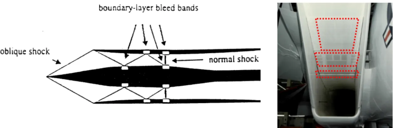
1.1 a) Axisymmetric mixed-compression inlet (M~2.5) with bleed bands for shock control, and b) F-15 external compression inlet (M~2.2) with the ramp bleed regions marked with red boxes... 7

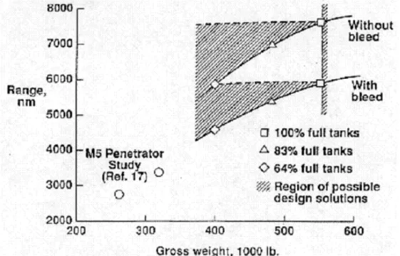
1.2 Range studies by Lockheed-Martin (Loth, 2000) for supersonic cruiser with and without bleed... 8

1.3 Streamwise vortices generated by the micro-vortex generators... 9

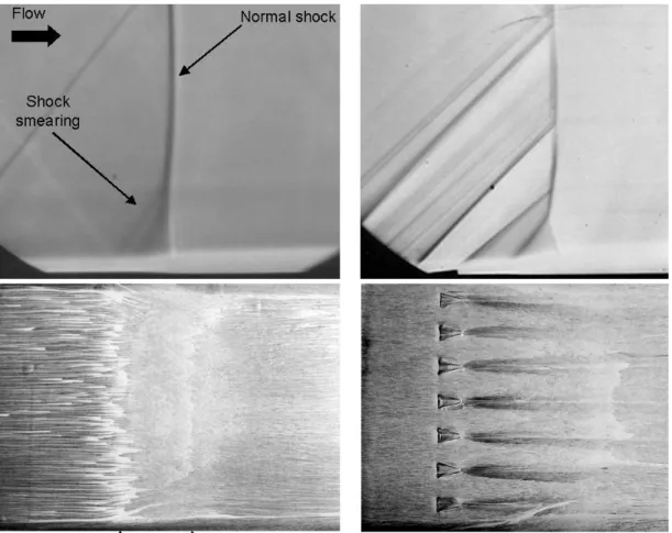
1.4 SBLI control with micro-vanes at M=1.5 by shadowgraph and oil-streak visualization with: no control (where “S” indicates separation and “R” indicates reattachment, b) flow with

micro-ramps... 10

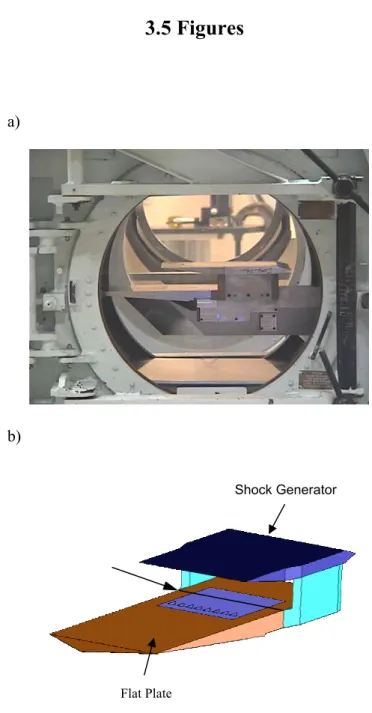
3.1 a) Flate plate with shock generator installed in TGF, b) Forebody Boundary Layer Management Model schematic... 34

3.2 Dimensions of baseline micro-ramp from Anderson et al. (2006)... 35

3.3 Boundary layer rakes a) schematic where holes represent Pitot probe positions (mm unit), b) an actual picture of the rakes... 36

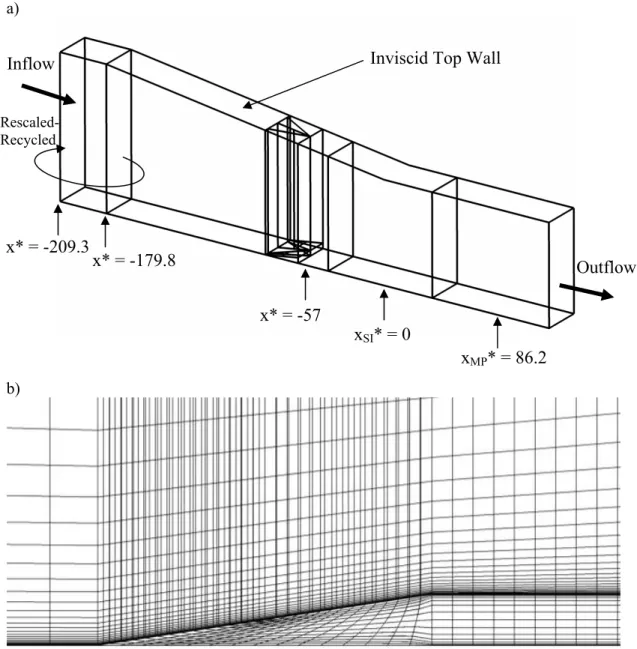
3.4 Grid topology for a) angled view of the whole domain, and b) zoom in at the micro-ramp... 37

3.5 Study of a) integral time convergence on velocity profile, b) grid resolution on velocity profile, c) integral time convergence on total pressure profile, and d) grid resolution on total pressure profile for baseline ramp... 39

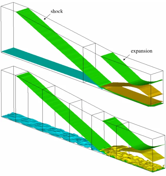
3.6 Iso-surface of density for NR where RANS shown on top and LES on bottom... 40

3.7 Visualization of various plane for NR z*=0 and at y+_{=1 from x*=-38 to +102: a) mid-span Mach} number contours for y*=0 to 69, and b) near-wall streamwise velocity contours for z*=-11.9 to +11.9. Note that the plane y+_{=1 corresponds to the first vertical grid point above the wall, which} was the same for all flows since this grid point was based on the NR shear stress at x*=-209.3.... 41

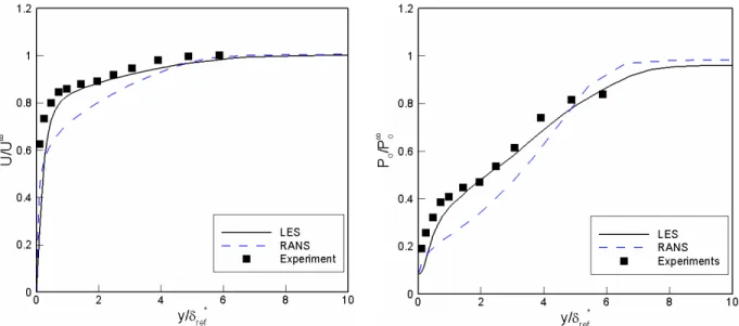
3.8 Streamwise velocity and total pressure profile comparison between RANS, LES and experimental data for NR at measuring plane (xMP*=86.2)... 42

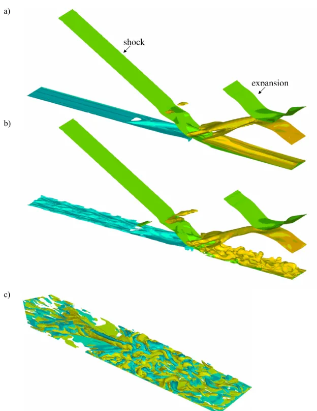
3.9 Iso-surface of a) density for averaged LES, b) instantaneous LES and c) streamwise vorticity of instantaneous LES... 43

(12)

3.10 Visualization of a) streamwise and b) spanwise planes for BR with same contours and domain as for Fig. 3.7. The solid arrow indicates the spanwise location of the streamwise contours while the two dashed arrows indicate the two streamwise positions shown in Fig. 3.11... 44 3.11 a) velocity contours at y+_{=5 for NR and b) velocity contours at y}+_{=5 for BR showing streamwise}

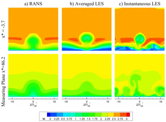
lengths of 8δ (400 wall units) and 20δ (1000 wall units) in the spanwise length... 45 3.12 Visualization of cross sectional plane Mach contours for BR at x*=-3.7 (near shock impingement)

and x*=86.2 (measuring plane) for a) RANS, b) averaged LES and c) and instantaneous LES.... 46

3.13 Comparison of streamwise velocity and total pressure profile for LES, RANS and experimental data for BR at x*=86.2 (measuring plane) for Rake 1 (z*=11.8), Rake 2 (z*=9.7) and Rake 3

(z*=7.5)... 47

3.14 RANS turbulence model comparison (Shear Stress Transport (SST), Spalart-Allmaras (S-A), Baldwin-Lomax (BL)) with LES and experimental data... 48

3.15 Visualization streamwise velocity from x*=-28.5 to 102 at y+_{=1 plane for BR, HR and HRHD for a)} averaged LES average and b) instantaneous LES... 49

3.16 Mach contours at various cross sections for BR, HR and HRHD: a) instantaneous LES at the micro-ramp’s trailing edge (x*=-57 for BR and HR and x*=-28.5 for HRHD), b) instantaneous LES at measuring plane and c) averaged LES at measuring plane... 50

3.17 Spanwise distributions of a) total pressure loss for BR and d) HR and HRHD, b) displacement thickness for BR and e) HR and HRHD, c) incompressible shape factor for BR and f) HR and HRHD at measuring plane, x* = 86.2, comparing with experimental data... 51

4.1 Various types of μVGs with length and width scaled with the height (h) where the spacing between the centerlines of the adjacent μVGs is 7.5h : a) baseline ramp (BR), b) half height ramp (HHR), c) half width ramp (HWR), d) split ramp (SR), e) baseline vane BV, f) thick vane (TV)... 70

4.2 Computational grid a) at z=0 with the domain dimensions and b) a side view of the μVG at

z=11.85δref*... 71 4.3 Streamwise velocity profile compared with experimental data4 at MP for a) NR and b) BR where

results for the baseline grid (BG), the dense grid (DG) and two different averaging time-scales are compared... 72

4.4 Flow visualization of oblique shock interaction: a) density iso-surface for NR, b) velocity contours at y+_{=5 for NR and c) velocity contours at y}+_{=5 for BR showing reference lengths of 1000}

streamwise wall units and 100 spanwise wall units... 73

4.5 Cross-sections of time-averaged (T*=4) streamwise velocity contour at the trailing edge of μVGs (x*= -57 with the center of the vortices are indicated by the arrows) and the inviscid shock location (x*= 0)... 74

4.6 Time-averaged streamwise velocity contour for a) spanwise view of flow separation region shown in dark for negative wall shear stress at y+_{=1 and b) streamwise view showing the oblique shock}

(13)

and the separation bubble (blue region) for x*=-57 to 19 at a spanwise location of z*=11.8

(consistent with the red arrow in Fig. 4.6a)... 75 4.7 Time-spatially averaged (for T*=4 from y*=0 to 4.66 and z*=0 to 4.66) values for pressure and

turbulent kinetic energy at discrete streamwise locations. Arrows indicate the SBLI regions... 76

4.8 Temporally and spatially averaged (same as Fig. 4.7) values for streamwise vorticity and the spatially averaged center that represents the path of the vortex pair for each μVGs. Arrows indicate the SBLI region... 77

4.9 Side view a) schematic of transverse path of the vortex tube with respect to the boundary layer (BL) edge with the oblique shock interaction, b) averaged density contour of BR case, top view of the streamwise velocity contours at y+_{=5 for c) BR and d) TV where the streamlines show the}

approximate trajectories of the primary vortices... 78

4.10 Correlation of a) circulation of various μVGs at 5h downstream with the device height in wall units and b) decay of vortex peak strength with downstream distance... 79

4.11 Spanwise distribution of stagnation pressure recovery, displacement thickness and incompressible shape factor for various μVGs, where δNR*/δref* = 1.07, αNR = 0.80 and HNR = 1.25. The incompressible shape factor from Ashill et al.(2002) data for a baseline micro-vane (Ashill Vane), which has the same dimensional scaling as Fig. 4.1e, is compared with the present LES result... 80

5.1 Computational domain beginning with the recycling zone (Lrec=26.6h) where the micro-ramp is placed at the middle of the domain with downstream extension of 57.9h... 98

5.2 Vorticity modulus at y+=25 for a turbulent boundary layer at M=3 with a coarse grid (CG) resolution for present simulations: a) min-mod 3rd order, b) superbee 3rd order, c) superbee 5th order. Also shown is d) Urbin et al. (1999) simulations with a similar coarse grid (CG) resolution using Reimann solver and 2nd /3rd order reconstruction functions... 99

5.3 Numerical scheme study based on the velocity and streamwise Reynolds stress profiles comparing with various supersonic experimental data and Urban et al. (1999) course grid results... 100

5.4 Vorticity modulus at y+_{=25 for different grid resolution are shown for a turbulent boundary layer at} M=3 a) course grid (Δx+ = 28, Δz+ = 13 and Δy+ = 1 with r = 15%), b) same as CG except Δx/2, c) same as CG except Δz/2 and d) same as CG except Δx/2+Δz/2... 101 5.5 Streamwise velocity contour at y+_{=8 for different grid resolution are shown for a turbulent}

boundary layer at M=3 a) same as CG except Δx/2, b) same as CG except Δz/2, c) same as CG except Δx/2 + Δz/2 and d) DNS of Martin (2007)... 102 5.6 Reynolds stress profiles in a) streamwise, b) transverse, c) spanwise direction are shown where grid

resolution sensitivity is studied and compared with Urbin et al. (1999) CG and DG profiles along with the experimental data of Konrad & Smits (1998). Mean velocity profiles are compared in similar fashion... 103

5.7 Mean velocity profiles comparisons of subsonic (Klebonoff 1954) and supersonic (Konrad & Smits 1998) experiments, theoretical prediction of White & Christoph (1991), Wu & Martin (2008) DNS data and LES using the baseline grid where close agreement is seen at the log-layer... 104

(14)

5.8 Streamwise view of instantaneous density contours at z=0 for a) M = 1.4 b) M=3.0 and velocity contours for c) M = 1.4 and d) M=3.0... 105 5.9 Wall surface pressure coefficient for a) M=1.4 experiments (Konrad & Smits 1998), b)

instantaneous LES predictions at M=1.4, c) M=2.2 and d) M=3.0... 106

5.10 Mach contours of instantaneous LES flow solution at y+_{=12 (above the floor and the top surface of} the micro-ramp) for a) M=1.4 and b) M=3.0... 107

5.11 Oil visualization for a) M=1.4 and b) M=2.5 are compared with instantaneous streamlines of LES c) for M=1.4 and d) M=2.2 where each micro-ramp heights are similar... 108

5.12 Spanwise view of instantaneous streamwise velocities are shown at various downstream locations for M=1.4 and M=3.0 using LES... 109

5.13 Low speed streaks (a, b) and vorticity modulus (c, d) for M=1.4 and M=3.0 at y+_{=25 are shown,} along with the shear stress coefficient (x1000) downstream of the micro-ramp (e, f)... 110 5.14 Spanwise view of streamwise vorticity along various downstream locations of the micro-ramp

showing different decay rate for M=1.4 and 3.0... 112

5.15 Spanwise view of turbulent kinetic energy shown at various downstream location of the micro-ramp where M=1.4 case have higher decay rate than the higher Mach number... 113

5.16 Spanwise averaged profiles of turbulent kinetic energy at upstream and downstream locations of the micro-ramp for different Mach number where the micro-ramp has the most impact on the lower Mach number case... 114

5.17 Correlation of circulation with respect to the effective height normalized in local wall units for various experiments and numerical simulation results... 115

5.18 Averaged streamwise vorticity a) decay along the streamwise direction and b) that normalized by the averaged streamwise vorticity at h downstream of the micro-ramp displayed in log units... 116

5.19 Vortex core trajectory for a) normal and b) spanwise distance for the experimental cases of Ashill et al. (2002) and Babinsky et al. (2009) and LES study at various Mach numbers... 117

6.1 a) schematic of a two dimensional computational domain and b) the mesh which used for RANS flow solutions... 138

6.2 RANS flow with a freestream Mach number of 1.4 and different diffuser lengths: a) 1.15L, b) 1.20L and c) 1.25L... 139

6.3 Mach profiles at the measuring plane for various diffuser heights and upstream Mach numbers... 140

6.4 Streamwise velocity contour showing the effects of the diffuser slope angle (5o_{and 7}o_{) and diffuser} shape (straight and sinusoidal curve where blue regions have a negative streamwise velocity (indicating flow separation) and red regions have a streamwise velocity at least 99% of the freestream velocity... 141

(15)

6.6 Schematic of a) the computational domain for large eddy simulation is shown which begins with the recycling zone and the μVGs are placed upstream of the shock, which sits in front of the inlet splitter plate (at x=0). b) Streamwise view of the LES grid... 143

6.7 Computational grid near a micro-ramped vane: a) top-view indicating the leading edge gap (gLE) and trailing edge gap (gTE) and b) side-view... 144

6.8 Various configurations of μVGs where spacing, length and width dimensions are specified relative to terms of device height (h) for; a) ramp (R2), b) split-ramp (SR2), c) ramped-vane (RV2, RV2U and RV3), d) ramped-vane with larger spacing (RV1) and e) ramped-vane with 50% size increase (RV1B)... 145

6.9 LES predictions with coarse (CG) and baseline-resolution (BG) for of a) mean stream wise velocity, b) Reynolds stress... 147

6.10 Time-averaged spanwise CG LES in the vicinity of the normal shock (x=-14.9δref to 2.1δref)

showing flow separation (negative wall shear stress) as the dark regions. The red arrows pointing to the left are the locations of the device trailing edge, except for RV2U whose trailing edge is at x=-18.4 δref (indicated by the long arrows)... 148 6.11 Spanwise view of streamwise vorticity at x=-12.3δref (just upstream of the shock interaction) based on time-averaged CG LES results for various devices... 149

6.12 Spanwise view of turbulent kinetic energy for various devices based on time-averaged CG LES results at the same positions as Fig. 6.10... 150

6.13 Spatially and time-averaged profiles at MP for various devices for: a) streamwise velocity b) turbulent kinetic energy and c) pressure RMS fluctuations... 151

6.14 Spanwise distribution of stagnation pressure recovery, displacement thickness and incompressible shape factor for various μVGs at MP... 152 6.15 Turbulent energy spectra of incoming streamwise velocity fluctuations for LES with baseline grid resolution compared with DNS spectra of Wu & Martin (2007)... 154

6.16 Spanwise view of streamwise vorticity at various locations downstream of RV1B for low and high resolution simulations... 155

6.17 Spanwise view of turbulent kinetic energy at various locations downstream of RV1B for low and high resolution simulations... 156

6.18 Instantaneous (INST) and time-averaged (AVG) streamwise velocity contours of NR and RV1B from coarse and baseline simulations over a streamwise distance of x=-18.4δref to 2.1δref where dark regions indicate negative wall shear stress... 157

6.19 Streamwise view of instantaneous (INST) and time-averaged (AVG) Mach contours of NR and RV1B at z=0 from coarse and baseline simulations over a streamwise distance of x=-18.4δref to 68.9δref. The red arrows are the RV1B positions... 158

(16)

6.20 Iso-surface of Mach contours at M=0.2 and M=1.2 of a) NR and b) RV1B where insets show a close up view near the shock... 159 6.21 Iso-surface of an instantaneous streamwise vorticity of a) NR and b) RV1B with insets showing a close up view near the shock and a downstream region... 160

6.22 Spanwise view of skin friction coefficient contours (x=-14.9δref to 68.9δref) where blue indicates flow separation for a) NR and b) RV1B... 161

6.23 Temporal and spatially averaged skin friction coefficient along downstream of the device for NR and RV1B where the shock region is indicated by the arrow... 162 6.24 Temporally and spatially averaged static pressure at the wall along downstream for NR and RV1B and the shock region is indicated by the arrow... 163

6.25 Pressure signals at (a) the wall and (c) y-ywall=8δref for NR and RV1B at upstream of the shock (x=-21.6δref) and MP (x=43.5δref). Pressure energy spectra are shown at the same streamwise locations at (b) the wall and (d) y-ywall=8δref... 164 6.26 Temporally averaged streamwise distribution of peak streamwise vorticity in terms of a) magnitude, b) transverse path and c) spanwise path. Black arrows indicate the SBLI region and the reds are the inlet location... 165

6.27 Spanwise distribution of stagnation pressure recovery, displacement thickness and incompressible shape factor for NR and RV1B at MP... 166

(17)

List of Tables

3.1 Dimension of the domain and the μVGs... 38

3.2 Spanwise Averaged Performance Parameters where αNR =0.80, δNR*= 1.09δref* (xSI), HNR=1.25 and Asep,NR=8.01Dδref* ... 52

4.1 Spanwise averaged performance parameters for different μVGs with Asep NR=8.01Dδref* ... 81

5.1 Reynolds number dependence on wall shear stress... 111

6.1 Definitions of acronyms for μVG configurations... 146

(18)

List of Symbols

a speed of sound

α total pressure recovery factor Asep separation area

β frictional velocity ratio BR baseline micro-ramp BV baseline micro-vane c cord length of the micro-ramp CFL Courant-Freidrichs-Lewy number

CG coarse grid

d width of the micro-ramp

δ boundary layer thickness

D width of the computational domain

DG dense grid

δref* reference displacement thickness at x=0 but with no shock effects

dt differential time

dx differential length in streamwise direction dy differential length in normal direction dz differential length in spanwise direction E height of the computational domain

γ specific heat ratio

Γ circulation induced by vortex generators h micro-ramp height

H incompressible shape factor

η wall normal coordinate normalized by boundary layer thickness HHR baseline micro-ramp with reduced height by half

HR baseline micro-ramp reduced in size by half

HRHD HR positioned at mid point between the BR and inviscid shock impingement location HWR baseline micro-ramp with reduced width by half

κ Von Karman constant

K spatial average of time-averaged turbulent kinetic energy L length of the computational domain

μ micro

M Mach number NR no micro-ramp

p time-averaged pressure

P spatial-average and time-averaged pressure Po total pressure

Reref Reynolds number based on δref*

(19)

s spacing between adjacent micro-ramps at the centerline SR BR split at the centerline

SBLI shock boundary layer interaction t fluid convection time scale

Δt time step T temperature

τ integration time for averaging

τ∗ _{integration time normalized by the freestream flow convection time}

TV thick vane

u instantaneous streamwise velocity u’ streamwise fluctuation velocity U average streamwise velocity Uτ frictional velocity

υω kinematic viscosity at wall

v transverse velocity VG vortex generators w width of the micro-ramp w spanwise velocity W weighting function

W average streamwise vorticity

ωmax maximum streamwise vorticity in a vortex core ωx streamwise vorticity

x streamwise distance

Δx streamwise length of computational cell

ξ i direction in computational domain y normal distance relative to solid-wall Δy transverse length of computational cell Y transverse trajectory of streamwise vorticity

ψ j direction in computational domain

z spanwise distance relative to center of domain Δz spanwise length of computational cell

Z spanwise trajectory of streamwise vorticity

ζ k direction in computational domain Superscripts

_

time-averaged + _{dimension in wall units} * _{dimension normalized by}_δ

ref*

** _{dimension normalized by h}

∞ freestream value

inner boundary layer inner region outer boundary layer outer region

Subscripts

dom domain

eddy turbulent eddies exit domain exit

f total integration time required for final convergence

(20)

∞ freestream value

inlet upstream plane used as input for recycling int total integration time

max maximum

MP measuring plane

rec downstream recycling plane SI theoretical shock impingement location TE μVG trailing edge location

(21)

Chapter 1 Introduction

The performance of supersonic engine inlets is critically affected by shock wave/boundary layer

interactions (SBLIs) occurring throughout the supersonic portion of the flow. Many of these interactions

are caused by oblique shock waves, but the final interaction is usually due to a normal shock. In all these

shock systems, the boundary layers growing along the walls of the intake are subjected to severe adverse

pressure gradients which can cause boundary layer separation, unsteady flow, and even engine un-start.

This chapter discusses flow control devices for SBLIs and provides motivations for the present study. A

review of previous work is also given. Finally, the chapter concludes with a statement of the objectives of

the present study.

1.1 Motivation

Currently, problems in SBLIs with flow separation and boundary layer unsteadiness are avoided

primarily through the use of boundary layer bleed/suction. This control method is able to suppress shock

induced separation and improve the boundary layer health if sufficient mass removal is employed. Bleed

can also fix the location of the final shock wave and help to prevent shock oscillations and flow

unsteadiness. Figure 1a shows the application of bleed to a mixed-compression inlet, while Figure 1b shows ramp bleed regions for a typical high-speed external compression inlet (this inlet also contains

additional side-wall and cowl bleed). The bleed is sometimes separated into “performance-bleed” and

(22)

while the second is designed to ensure normal shock stability. However, many forms of bleed in current

inlets satisfy both goals.

However, bleed mass flow rates have to be considerable to achieve the desired control effect (often

10-20% of intake mass flow). Such a large removal represents a source of significant vehicle performance

degradation because of the lost engine mass flow, the over-sizing of the inlet, and the effective drag

associated with bleed. As such, several design studies have shown that the bleed penalty on overall

performance can be significant. For example, trade studies completed by Lockheed-Martin (Loth 2000)

have shown that large range increases (on the order of 20%) are possible if bleed could be completely

eliminated as shown in Fig. 2. Similarly, Boeing Phantom Works conducted trade studies which indicated

that the gross total over weight (GTOW) can be reduced by as much as 10% if bleed mass flow could be

eliminated without degrading inlet performance (Loth 2000). Therefore, it would be highly advantageous

to devise a flow control system which gave the SBLI benefits of bleed but did not incur the penalties

associated with the mass removal.

It is the intention of this study to investigate novel types of flow control that may be able to offer

similar control benefits without the need for bleed. As long as these gains are achievable with negligible

drag increase and possibly increased shock stability, the overall advantage of such flow control system

could be highly significant. Perhaps a more likely scenario for future inlet flow control is that bleed will

be reduced (instead of eliminated) when coupled with effective zero-transpiration SBLI control systems.

Thus, in either case, techniques that can allow the advantages of bleed on boundary layer health and

stability during shock interactions without the mass flow rate loss are highly desirable.

1.2 Previous Studies

Several new approaches have been suggested in recent years which have significant potential for

SBLI control as discussed in the reviews by Raghunathan (1988) and Srinivasan et al. (2006). Vortex

(23)

interactions in internal flows. These devices introduce upstream streamwise vorticity into a flow field to

delay or suppress flow separation. Traditional vortex generators, however, have a large drag penalty due to their size and are not ideal for use inside inlets due to their mechanical vulnerability. Holmes et al.

(1987) suggested that smaller VGs can produce benefits similar to those of traditional VGs while having

greatly reduced parasitic drag. These smaller VGs are characterized by heights less than the boundary

layer thickness and have been referred to as “low-profile” or “micro” VGs, where in particular,

micro-vanes and micro-ramps are shown in Fig. 3. Meso-scale versions (smaller than the boundary layer

thickness but of the same order in size) were investigated by McCormick (1993) with encouraging results.

Micro-devices (much smaller than the boundary layer thickness), may have a significantly reduced

viscous drag penalty since they are well embedded and below most, if not all, of the supersonic portions.

The potential of micro-devices for supersonic inlet flow control has been investigated via various

SBLI configurations. For example, experiments in the NASA Unitary Plan Wind Tunnel with a full M=2

external-compression inlet showed that small flexible flaps improved stagnation pressure recovery,

reduced unsteadiness, and increased mass flow rate as compared to solid walls (Loth et al. 2004). This is

consistent with simulations and small-scale experiments whereby normal and oblique shock flows were

shown to be improved significantly with small-scale flow control (Loth 2001, Gefroh et al. 2002,

Hafenrichter et al. 2002, Kim et al. 2003). Recent work has focused again on vanes and

micro-ramps as they are physically robust, while still allowing a significant impact on SBLI flows. For example,

in an experimental study of normal SBLIs at Mach 1.5, micro-ramps have been shown to considerably

reduce separations while micro-vanes have been demonstrated to completely eliminate separation (Holden and Babinsky 2006). An example of the latter is shown in Fig. 4.

On transonic airfoils, micro-ramps have been shown experimentally to reduce shock strengths and

delay shock induced separations (Ashill et al. 2001) with significantly reduced device drag when

compared to traditional VGs. More recently, RANS computations performed by NASAGlenn Research

Center (Anderson et al. 2006) on inlet configurations, have demonstrated that micro-ramps have the

(24)

offering practical advantages such as physical robustness, low-cost and no power requirements. He

optimized the size and relative length scales of the device based on the downstream incompressible shape factor using RANS numerical methods.

However, the above control methods are not yet fully understood at a fundamental level. Initial

mean-flow measurements and Reynolds-Averaged Navier-Stokes studies have raised a number of questions as

to the detailed flow structure downstream of such devices, which is small-scale, highly three-dimensional,

and unsteady, but yet uncharacterized. This lack of basic understanding makes it impractical to optimize

their application to a real problem and define, for example, the ideal location and number of devices as

well as their optimum size/strength. Thus, the potential for bleed reduction/elimination and possible

performance gains have not been quantified with high fidelity. To date there have been only a few

systematic experimental and LES studies comparing different types of μVG flow control methods in conjunction with flow-fields representative for supersonic inlets. Ghosh et al. (2008) used a hybrid

Reynolds Average Navier-Stokes / Large Eddy Simulations (RANS/LES) with an Immersed Boundary

Method (IBM) to study oblique shock interactions with micro-ramps. Their RANS/LES approach is

helpful in that it allows much higher Reynolds numbers than are practical to compute with an LES.

However, the role of the turbulence model empiricism is increased as compared to LES. Their IBM

approach is computationally efficient because the grid does not need to conform to the ramps and does

not require fine normal spacing on the surface of the ramps. However, their approach yields a

wall-function like description of the micro-ramp boundary layers which may miss some important detailed

flow features that would be captured by an LES approach with body-fitted grids.

1.3 Objectives of the Present Study

The proposed Large-Eddy Simulation (LES) technique has been shown to provide details of the eddy

structure with high-fidelity of the mean and turbulence properties of supersonic turbulent boundary layers.

(25)

basic SBLIs which represent the canonical flows in supersonic inlets. Emphasis will be placed on

examining fundamental aspects of turbulent interactions with the generated streamwise vorticity, separation bubble dynamics and character, and boundary layer recovery and health. The resulting

investigation will allow direct evaluation of the efficacy of the μVG’s for SBLIs with respect to the three primary performance functions:

i) ability to improve separation reduction (decrease bleed mass rate and/or distortion)

ii) ability to improve stagnation pressure characteristics (increase recovery)

iii) ability to improve boundary layer health (decrease susceptibility to downstream

adverse pressure gradients caused a subsonic diffuser)

Such an integrated assessment is unprecedented and important, as the gains that could be achieved by

better flow management through novel control could be substantial. Chapter 3 investigates micro-ramps

under an oblique shock condition with a freestream Mach number of 3. Three different micro-ramp

configurations are simulated to assess the impact of ramp size and its position on overall performance as

measured by total pressure recovery, boundary layer growth, and incompressible shape factor of the

boundary layer downstream of the interaction. Chapter 4 presents results on further variations of the

geometry of the flow control device to understand how the development of the vortices differs between

various device geometries and compare that to previous subsonic measurements (Ashill et al. 2002).

Furthermore, the evolution of the turbulent eddies passing over the μVGs and their impact on the oblique shock is investigated. Finally, the downstream boundary layer properties are compared with the results of

different devices. Chapter 5 investigates the Mach number effect on flow traveling over the micro-ramp at

three different Mach numbers of 1.4, 2.2 and 3.0, but with no shocks. The impact of micro-ramps on the

turbulent boundary layer with respect to the high-speed fluid entrainment, the wake effects and the

(26)

counter-rotating vortices and their mean trajectories are compared as well. Lastly, Chapter 6 presents similar

studies with the various types of flow control device, but under normal shock conditions with a subsonic

diffuser. Course resolution results using different μVGs are compared to select the optimum candidate which is then simulated on a high-density grid to evaluate the device performance at the diffuser.

(27)

1.4 Figures

Fig. 1.1 a) Axisymmetric mixed-compression inlet (M~2.5) with bleed bands for shock control, and b) F-15 external compression inlet (M~2.2) with the ramp bleed regions marked with red boxes

(28)

Fig. 1.2 Range studies by Lockheed-Martin (Loth 2000) for supersonic cruiser with and without bleed

(29)

(30)

Fig. 1.4 SBLI control with micro-vanes at M=1.5 by shadowgraph and oil-streak visualization with: no control (where “S” indicates separation and “R” indicates reattachment), b) flow with micro-ramps

(31)

Chapter 2 Numerical Methodology

2.1 Governing Equations

The governing fluid dynamic equations are often put into nondimensional form. The

advantage in doing this is that the characteristic parameters such as Mach number, Reynolds

number, and Prandtl number can be varied independently. Also, by nondimensionalizing the

equations, the flow variables are “normalized”, so that their values fall between certain

prescribed limits such as 0 and 1. The nondimensional coordinates and the primitive and

thermodynamic variables are shown in the following:

*

x

L

=

* y y L = * z z L = * / t t L U_∞ = * u u U_∞ = * v v U_∞ = * w w U_∞ = *

μ

_∞ = *

ρ

_∞ = * 2 p p U

ρ

_∞ _∞ = * T T T_∞ = * 2 e e U_∞ = (2.1) where the non-dimensional variables are denoted by an asterisk, freestream conditions are denoted by ∞,

and L is the reference length used in the Reynolds number:

ReL U L

ρ

μ

∞ ∞ ∞ = (2.2)

(32)

If this non-dimensionalizing procedure is applied to the compressible Navier-Stokes equations, the

following nondimensional equations are obtained. Note that the asterisks are dropped for convenience.

0 U

E

F

G

t

x

y

z

∂

₊

∂

₊

∂

₊

∂

₌

∂

_(2.3) where U, E, F and G are the vectors of

t u U v w E

ρ

⎡ ⎤ ⎢ ⎥ ⎢ ⎥ ⎢ ⎥ = ⎢ ⎥ ⎢ ⎥ ⎢ ⎥ ⎣ ⎦_(2.4) 2 ( ) xx xy xz t xx xy xz x u u p E uv uw E p u u v w q

ρ

τ

ρ

τ

ρ

τ

⎡ ⎤ ⎢ ⎥ + − ⎢ ⎥ ⎢ ⎥ = − ⎢ ⎥ ⎢ − ⎥ ⎢ ⎥ + − − − + ⎢ ⎥ ⎣ ⎦_(2.5) 2 ( ) xy yy yz t xy yy yz y v uv F v p vw E p v u v w q

ρ

τ

ρ

τ

ρ

τ

⎡ ⎤ ⎢ ₋ ⎥ ⎢ ⎥ ⎢ ⎥ =_⎢ + − _⎥ ⎢ ₋ ⎥ ⎢ ⎥ + − − − + ⎢ ⎥ ⎣ ⎦_(2.6) 2

(

)

xz yz zz t xz yz zz z

w

uw

G

vw

w

p

E

p w u

v

w

q

ρ

τ

ρ

τ

ρ

τ

⎡

⎤

⎢

⎥

−

⎢

⎥

⎢

⎥

=

_⎢

−

_⎥

⎢

_{+ −}

⎥

⎢

⎥

+

−

+

⎢

⎥

⎣

⎦

_(2.7) and

(33)

2 2 2

2

t

u

v

w

E

=

ρ

⎛

_⎜

e

+

+ +

⎞

_⎟

⎝

⎠

_(2.8) The components of the shear-stress tensor and the heat flux vector in nondimensional form are given by

2

2 3Re

xx L

u

v

w

x

y

z

μ

τ

=

⎛

_⎜

∂

−

∂

−

∂

⎞

_⎟

∂

⎝

⎠

_(2.9)

2

2 3Re

yy L

v

u

w

y

x

z

μ

τ

=

⎛

_⎜

∂

−

∂

−

∂

⎞

_⎟

∂

⎝

⎠

_(2.10)

2

2 3Re

zz L

w

u

v

z

x

y

μ

τ

=

⎛

_⎜

∂

−

∂

−

∂

⎞

_⎟

∂

⎝

⎠

_(2.11)

Re

xy L

u

v

y

x

μ

τ

=

⎛

_⎜

∂

+

∂

⎞

_⎟

∂

⎝

⎠

_(2.12) Re xz L u w z x

μ

τ

= ⎛_⎜∂ +∂ ⎞_⎟ ∂ ∂ ⎝ ⎠_(2.13)

Re

yz L

v

w

z

y

μ

τ

=

⎛

_⎜

∂

+

∂

⎞

_⎟

∂

⎝

⎠

_(2.14) x ( 1) 2Re PrL T q M x

μ

γ

_∞ ∂ = − − ∂ _(2.15) ( 1) 2Re Pr y L T q M y

μ

γ

_∞ ∂ = − − ∂ _(2.16) ( 1) 2Re Pr z L T q M z

μ

γ

_∞ ∂ = − − ∂ _(2.17)

where M∞ is the freestream Mach number,

U

M

RT

γ

∞ ∞ ∞

=

(2.18)

(34)

p

=

ρ

RT

(2.19)

WIND code (developed at AEDC and NASA Glenn) solves the above compressible

Navier-Stokes equation with the cell-vertex finite volume formulation. In the following section,

turbulence closure and the inflow boundary condition are discussed in detail.

2.2 Numerical Techniques

2.2.1 Large Eddy Simulation

The computational effort consists of Large Eddy Simulations (LES) which provide fine spatial and

temporal resolution of the turbulent structures. The WIND code was used to make the LES computations.

The monotone integrated LES (MILES) technique based on Furbey and Grinstein(1999) solves the

unfiltered Navier-Stokes equations using high-resolution monotone algorithms. The convection

discretization (high order upwind is used in the present study) acts as a filter for the nonlinear

high-frequency modes to dissipate the kinetic energy accumulated at high wave numbers, thus dispensing the

need to use an explicit subgrid-stress modeling. Studies (Furbey and Grinstein, 1999) of the forced homogeneous isotropic turbulence showed that the simulated energy spectra depend on the effects of the

subgrid-stress model only toward the high-wave number end of the inertial range and into the viscous

subrange. The LES becomes significantly independent of the subgrid-stress model if the resolution has a

cutoff wave number that lies in the inertial subrange. In addition, the effect of subgrid-stress modeling

may be less significant in supersonic flows which contain shock-waves since the limiters used to resolve

the shocks are themselves significantly diffusive. For example, the effect of a sub-grid model was found

to be very weak in the LES study by Urbin et al. (1999) on supersonic turbulent boundary layers, despite

the use of a high-accuracy Riemann scheme. In particular, the MILES results gave close agreement with

that using a Smagorinsky subgrid-stress model (1963), indicating that the sub-grid model had little impact

(35)

turbulent boundary layer using the WIND code. Therefore, the present study employed “Large Eddy

Simulation without a subgrid stress model”, (LES-nSGS).

2.2.2 Rescale-Recycling Method

The rescale-recycling method, originally developed by Lund et al.(1998) for incompressible flows,

has been extended for compressible boundary layer flows by Urbin et al.(1999, 2000). The result is a

computationally efficient method of generating turbulent inflow condition by eliminating the need to

simulate boundary layer flows from the leading edge of the flat plate, through transition. For the

recycling method, the instantaneous flow field at a given downstream location is rescaled using boundary

layer theory to match the average flow field at an upstream recycle location, where it can then be used as

an input for another cycle. The downstream plane will be denoted the “recycle” plane and the upstream

plane will be denoted the “inlet” plane. This technique requires that the distance between the two

recycling stations is sufficiently long; i.e. x+_{of 1000 wall units}_(Urbin_{et al.}_{2000). Multilayer scaling}

(

Kistler and Chen 1963)

can be used for the boundary layer profile and we decompose it into an inner and outer layer, similar to Urbin et al.(1999, 2000). The time- and spanwise- average streamwise velocity

(U) can be used to obtain the frictional velocity at the wall from which the inner layer velocity profile

(Uinner_{) can be described in terms of the law of the wall:}

0 0 1 D f f U udtdz D τ τ =

_{∫ ∫}

(2.20) 1 ( ) ( ) inner U U x_τ n y C κ + ⎡ ⎤ = _⎢ + _⎥ ⎣ A ⎦ (2.21)

In the first expression, u is the instantaneous streamwise velocity, D is the width of the domain, and τf is the total integration time required for convergence. In the second expression, κ is the von Karman constant, and C is an empirical constant. Since Uτ is assumed to be only a function of the streamwise

(36)

coordinate, x, the average streamwise velocity at the inlet station can be obtained by multiplying the

frictional velocity ratio, β.

( )

inner inner

inlet recycle inlet

U =βU y+ (2.22)

In this expression, β = Uτ, inlet / Uτ, recycle. Note that Urecycleinner has been interpolated to the y+ coordinate system at the inlet station. The outer layer follows the velocity defect law such that the following similarity rule

can be applied.

( ) ( )

outer

U∞ −U =U x f_τ η (2.23)

where η = y / δ and δ is the boundary layer thickness. Similarly, outer layer of U at the inlet station can be obtained by

( ) (1 )

outer outer

U =βU η + −β U∞ (2.24)

where outer recycle

U is interpolated to the η coordinate system at the inlet station. As for the fluctuation velocity,

u’=u-U, where u is the instantaneous streamwise velocity, the rescaled fluctuation velocities for the inner

and the outer layer are obtained from the following equations.

'inner 'inner ₍ _{, , )}

u ₌βu y+ z t _(2.25)

'outer 'outer ₍ _{, , )}

u =βu η z t (2.26)

The composite equation is then obtained by combining the inner and the outer region of the boundary

layer profile using the weighting function.

' '

( inner inner )[1 ( )] ( outer outer ) ( )

inlet recycle recycle inlet recycle recycle inlet

u =β U +u −W η +β U +u W η (2.27)

where the weighting function (Urbin et al. 1999) is defined as

1 4( 0.2) ( ) 1 tanh / tanh(4) 2 0.6 0.2 W η η η ⎡ ⎛ − ⎞ ⎤ = _⎢ + _⎜ _⎟ _⎥ + ⎝ ⎠ ⎣ ⎦ (2.28)

(37)

Rescaling the wall normal (transverse) velocity, v, and the temperature, T, involves similar procedures

except for setting β = 1. β is set to the same value as the u case for spanwise velocity, w. The pressure at the inlet is assumed to be constant due to negligible fluctuations (

Kistler and Chen 1963)

. Thus, the density field at the inlet station can be computed directly from the rescaled temperature. Note that the

above method slightly differs from that of Urbin et al. (1999, 2000) with respect to Eq. 2.22 and 2.24.

Van Driest transformation applied to the mean streamwise velocity profile (Urbin et al. 1999, 2000)

requires a priori knowledge of the mean profile which is difficult to obtain for the present low Reynolds

number case. On the other hand, eliminating the transformation allows β to be factored out in Eq. 2.27 such that the instantaneous velocity profile at the recycling plane can be used directly. Xu and Martin (2004) have shown that even a pure periodic coupling between the inlet and the recycling plane yields

good agreement with the results from the rescale-recycling scheme similar to Urbin et al.(1999, 2000),

thus the present method was deemed appropriate.

To rescale the flow field at the recycle station to the inlet station coordinate, yinlet+ and ηinlet, the

boundary layer thickness ratio and the frictional velocity ratio must be computed a priori. These values

can be estimated from empirical relations given by Smits and Dussauge (1996) for the inner region

rescaling: 1 10 , , recycle inlet recycle inlet U U τ τ δ δ ⎛ ⎞ = ⎜ ⎟ ⎝ ⎠ _(2.29)

(38)

Chapter 3 Oblique Shock Boundary Layer Interaction and

Micro-Ramps

In the first part of the present study, we consider a Mach 3 turbulent boundary layer with a modest

Reynolds number to allow a LES approach. In particular, the Reynolds number based on the reference

incompressible displacement thickness, δref*, is about 3,800, where the freestream pressure and the

temperature are 7076 N/m2 and 582.3 K, respectively. Note that δref* in this chapter is the displacement

thickness that occurs at the theoretical inviscid shock impingement point, xSI, for a flat plate with no

shocks and no micro-ramps. LES was used to simulate a flat-plate / oblique shock interaction with and

without upstream micro-ramps. Three different micro-ramp configurations are simulated to assess the

impact of ramp size and its position on overall performance as measured by total pressure recovery, boundary layer growth, and incompressible shape factor of the boundary layer downstream of the

interaction.

3.1 Experimental Methodology

The experiments were conducted in the Air Force Research Laboratory’s (AFRL) Trisonic

Gas-dynamics Facility (TGF) (Clark 1982) at Wright Patterson Air Force Base on the Forebody Boundary

Layer Management (FBLM) model (Fig. 3.1). The TGF is a continuous circuit tunnel with a two square feet test section capable of operating in the subsonic, transonic and supersonic regimes. The model

consists of a beveled flat plate with an attached shock generator mounted on a strut so that the plate was

(39)

tunnel Schlieren window. Standard boundary layer transition calculations predicted transition within 20

mm of the leading edge, which is 559 mm upstream of the shock interaction, so no artificial trips were used. As shown in Fig. 3.1b, the oblique shock generated from the 8o_{shock wedge, impinged on the flat}

plate just upstream of the shock generator side-wall mounts. This configuration eliminated any sidewall

separation typical of a grazing wall shock. The boundary layer then propagates downstream to several

boundary layer rakes where the total pressure of the disturbed boundary layer was measured.

3.1.1 Experimental Test Conditions and Micro-Ramp

Data was collected at a nominal Reynolds number of 4,000 based on the reference displacement

thickness, δref*. Because δref* was not measured at xSI, its value was obtained from RANS flow

simulations. The Mach number in the test section was nominally 2.98 with a total pressure of 24,000

N/m2_{. Tunnel total temperature was maintained at approximately 300K. Total pressure was held constant}

through out the test. The height of the micro-ramp, h, was 2.82 mm and the reference displacement

thickness, δref*, was 0.88 mm, so that h=3.19δref*. Dimensions of the baseline micro-ramp are shown in

Fig. 3.2. The ramps are a design by Anderson et al. (2006) which is based on an investigation of different

shapes using RANS simulation. The micro-ramp flow control was machined into a plate that affixed to

the base for quick and easy model changes.

3.1.2 Instrumentation

Data extraction was based on boundary layer Pitot total pressure measurements and several static

pressure measurements. The static pressure rise observed through a shock interaction was only obtained

for the baseline oblique shock cases where micro-ramps were not present. The model insert plate that

contained the flow control devices was replaced with an insert containing an array of static pressure taps

with the first tap located 88.9 mm upstream of the inviscid shock location. This plate is known as the

“shock instrumentation plate”. Several rows of pressure taps were located in the region of the interaction

(40)

in front of each boundary layer rake at the measurement plane. Located 76.2mm downstream of the

inviscid shock location were four boundary layer rakes which were evenly spaced at 19.05 mm on one side of the centerline. Another one was located on the other side to ensure that the flow field was

symmetric. A total of twelve hypodermic Pitot tubes were placed in each rakes (Fig. 3.3a & b). The five

lower tubes have a 0.00063 mm outside diameter with a 0.00032 mm inside diameter and the upper 7

tubes have an outside and inside diameter of 0.00087 mm and 0.00047 mm, respectively. The two

columns of tubes have a lateral separation of 0.0014 mm.

The faces of all the tubes are cut square. The faces of the lower nine tubes are 0.004 mm from the

sharp leading edge of the support blade and for the upper three tubes, this distance is 0.008 mm. The

support blade has a leading edge angle of 40 degrees and a width of 0.0025 mm. The Pitot pressure data

were reduced to total pressures upstream of the tubes by an iterative solution of the Rayleigh Pitot

equation. Constant static pressure in the measurement region is based on Schlieren images which showed

that the flow after the shock interaction did not contain significant gas dynamic interactions. Rake data

and Schlieren images for the no shock case showed a small separation bubble at the base of the boundary

layer rakes. This separation impacted the lower three boundary layer rake probes and contaminated the

static tap just forward of the boundary layer rakes. Therefore, the data were reduced to using static tap

data from either the most downstream static tap on the shock instrumentation plate which was 40 mm

upstream of the boundary total pressure measurement plane or from a tap added to the micro-ramp flow

control plate 5 mm forward of the boundary layer Pitot pressure measurement plane. The baseline

boundary layer profiles, discarding the lower three probes due to the small separation bubble, fit well to a 1/7th_{power profile indicating a fully developed turbulent boundary layer. The repeatability error was}

(41)

3.2 Numerical Methodology

3.2.1 Numerical Schemes and Turbulence Models

The LES studies were conducted with and without micro-ramps at flow conditions closely matching

those of experiments at AFRL. The moderate Reynolds number of the experimental condition allowed

practical LES resolutions and run times. A third-order upwind (Courant et al. 1954) option, combined

with a min-mod limiter (Roe 1986) and a high-resolution structured grid were used to obtain high-fidelity

eddy structure and shock interactions simulations. The temporal integration used a second order, implicit, approximate factorization scheme (Holtz 1997) and Newton sub-iterations at each time step. The LES

approach was used to capture the turbulence effects.

The time step used for the LES study is Δt=CFLΔx/(a∞₊_U∞_{), where}_Δ_x_{is the streamwise cell length in}

the recycling zone and a∞_and_U∞_{is the speed of sound and streamwise velocity at freestream. The}

Courant number, CFL, was set to 0.4. Several conventional RANS models were examined for

comparison (including Spalart-Allmaras and Menter SST) but the differences were not significant. The

simple Baldwin-Lomax turbulence model was found to converge rather quickly (and was representative

of the other RANS models) and thus is shown for comparison in the below results with a CFL based on

the streamwise cell length of 0.8. However, comparison among all three turbulence models will also be

shown for a sample case with a baseline micro-ramp and a shock interaction.

Rescale-recycling method was used to generate incoming turbulent boundary layer (Urbin et al. 1999,

2000) and it was found that the recycling frequency is large enough to become decoupled with the

separated flows induced by the oblique shock. Fluid convection time scales can be based on the

freestream velocity and the convection length, e.g. this time-scale for the recycling zone is given by τrecycle=Lrecycle/U∞. The Lagrangian integral time scale of a turbulent eddy, τeddy, in a boundary layer can be

computed using the following equation (Loth 2010).

2

min (10 0.4 ) ,0.2

eddy w y Uτ Uτ

τ ₌ _⎡υ ₊ + δ _⎤

(42)

where υω is the kinematic viscosity at the wall, y+ is the normal distance in wall units and Uτ is the

frictional velocity. The eddy time-scale was found to be approximately 2.5 times smaller than the recycle

fluid convection time scale, i.e. τeddy/τrecycle~0.4. Therefore, the periodic recycle time-scale is significantly large compared to that associated with turbulent structures for the present simulations, as was also the

case for Urbin et al. (1999).

3.2.2 Computational Domain

As shown in Fig. 3.4a, the computational domain consists of 11 zones. The zones are required to grid

the complex geometry of the micro-ramp and an oblique shock wedge of angle, γ. The dimensions of the domain are based on the height of the micro-ramp, h, and the reference displacement thickness, δref*,

yielding a ratio of 3.19 which is the same as the experiment. The geometry of the micro-ramp is shown in

Fig. 3.2 and is defined to be the baseline micro-ramp configuration. The computational domain, shown in

Fig. 3.4, is a scaled version of the test section (Fig. 3.1) of the wind tunnel at AFRL. The length of the

domain is 312δref* (11,052 in wall units) and the width of the domain is 23.7δref* (840 in wall units) where

the spanwise coordinate, z, is defined as 0 at the centerline of the computational domain. The height

varies from 86.3δref* to 61.1δref* (3055 to 2164 in wall units) at the entrance and the exit of the domain.

The streamwise distance was normalized by the displacement thickness and centered at the theoretical

shock impingement location as x*=(x-xSI)/δref*. The micro-ramp trailing edge is located at x* = -57,

which is upstream of the shock impingement location. The first zone (recycling zone), whose length is

29.5δref*, generates turbulent boundary layer inflow conditions using the rescale-recycling method. The

supersonic flow enters into the test section where the wedge (γ = 8o) is placed at the top ceiling generating a 25.6 degree shock wave. The measuring plane (xMP) is located at x* = 86.2, which corresponds to the

location of the Pitot probes in the experiment, as shown in Fig. 3.4a. The no-slip condition is imposed on

the bottom plate and the micro-ramp, whereas the top ceiling has inviscid wall conditions. Periodic

Large eddy simulation of shock boundary layer interaction control using micro-vortex generators