Aerodynamic characterization of a Griffith-type transonic, laminar-flow airfoil

(1)

c

(2)

AERODYNAMIC CHARACTERIZATION OF A GRIFFITH-TYPE TRANSONIC, LAMINAR-FLOW AIRFOIL

BY

ARMANDO R. COLLAZO GARCIA III

THESIS

Submitted in partial fulfillment of the requirements for the degree of Master of Science in Aerospace Engineering

in the Graduate College of the

University of Illinois at Urbana-Champaign, 2019

Urbana, Illinois

Adviser:

(3)

Abstract

An experimental investigation was conducted at the University of Illinois’ Transonic Wind Tunnel Facility on a Griffith-type transonic airfoil to evaluate the effectiveness of its laminar flow qualities and boundary-layer flow-control characteristics in the transonic regime. Airfoil surface and wake pressure data were acquired to characterize the aerodynamic performance across a range ofα= -2◦−2◦andM=0.3−0.7. In addition, surface-oil flow visualization, PIV, and Schlieren imaging were performed to identify the suction influence on boundary-layer transition, momemtum deficit alleviation in the wake, and stability of transonic shocks.

It was observed from the pressure distributions that the flow control application had a beneficial influ-ence, allowing for a more aggressive pressure recovery downstream of the suction slot resulting in higher recovery pressure values at the trailing edge. At the design conditions of M = 0.7 andα= 0◦, a net pro-file drag reduction of 10.70% and an increase in the L/Dratio of 14.68% were observed when compared to no-suction conditions. Velocity flow field contours obtained from the PIV data showed an increase in the wake velocity magnitude for all Mach numbers atα=0◦, displaying excellent agreement for the drag data at these conditions. Surface-oil flow visualization experiments revealed that the airfoil experienced extensive laminar flow runs regardless of suction application due to the low-Reynolds number test condi-tion. The laminar flow was found to be shock limited followed by a laminar separation bubble in most cases. From the Schlieren experiments, a characteristic frequency of 22.38 Hz for the shock oscillatory process was identified at the design conditions which also was observed to stabilize under the influence of suction. In general, the improvements in aerodynamic efficiency and stability of the shock resulting from suction were observed to be greatest at higher angles of attack where the boundary layer was subjected to stronger-unforced pressure gradients.

(4)

To Mario and Wanda. Soli Deo gloria.

(5)

Acknowledgments

I would like to first thank my parents, Mario and Wanda, for their unwavering support throughout my life without which I wouldn’t be here. In particular, for supporting the desire of a 15-year-old to become a pilot which led to my current endeavors. Much appreciation goes to Bob Vargas for all the valuable life lessons which began at the golf course many years ago. I am also grateful for the guidance of Dr. Luis Gonzalez Linero and Dr. Rafael Rodriguez, both of whom helped guide me through my undergraduate studies and introduced me to research. Also, a special thanks goes to astronaut Sam Gemar for his help and advice as I made the decision to pursue graduate studies.

The family I have gained at the University of Illinois has made my graduate school experience worth-while. I will forever be grateful to the Aerospace Engineering department for the opportunity of being a student here and for the liberty I have been given to explore my interests in aerodynamics. I am also thank-ful for the unconditional help and support I have received from all of my labmates. Thanks to Rohit Gupta, Georgi Hristrov, and Prateek Ranjan for great camaraderie and for sharing many ups and downs these past two years. Also, thanks to Emily Weerakkody for great input during my writing process.

Last but foremost, I would like to deeply thank my advisor Dr. Phillip J. Ansell for believing in me and allowing me to be part of the Aerodynamics and Unsteady Flows Research Group. Especially for the guidance, technical conversations, and countless hours in the lab from which I have learned more about aerodynamics than in any class I have ever taken.

(6)

List of Tables

2.1 Reand volumetric flow rate for the Griffith airfoil based on corresponding Mach number. . . 31

4.1 Aerodynamic performance summary for all angles of attack at M = 0.3. . . 78

4.6 Averaged shock locations from flow visualization experiments for suction and no-suction cases. . . 82

4.7 Shock oscillatory frequency and averaged shock location summary from Schlieren data at M= 0.7. . . 83 B.1 Example of uncertainties for experimental measurements atM= 0.7,α=0◦, and no-suction. 98

(9)

List of Figures

2.1 Transonic Wind Tunnel Facility at UIUC. . . 32

2.2 NotionalC_p distribution for a transonic airfoil at three different design conditions . . . 32

2.3 Griffith-type transonic, laminar-flow airfoil profile. . . 33

2.4 Griffith-type transonic, laminar-flow airfoil seen inside the wind tunnel test section. . . 33

2.5 RAE 2822 airfoil profile modified with finite trailing edge. . . 34

2.6 RAE 2822 airfoil seen inside the wind tunnel test section. . . 34

2.7 Wake traverse system mounted in wind tunnel for wake pressure acquisition. . . 35

2.8 PIV setup in transonic wind tunnel. . . 35

2.9 One-mirror Schlieren setup schematic. . . 36

2.10 Experimental Schlieren imaging setup in the transonic wind tunnel. . . 36

2.11 Griffith airfoil in suction configuration setup prior to a flow visualization run. . . 37

2.12 Flow visualization image recording setup in transonic wind tunnel. . . 37

3.1 Cpdistribution forM= 0.3 atα=2◦. . . 50 3.2 C_pdistribution forM= 0.4 atα=2◦. . . 50 3.3 Cpdistribution forM= 0.5 atα=2◦. . . 50 3.4 Cpdistribution forM= 0.6 atα=2◦. . . 50 3.5 Cpdistribution forM= 0.7 atα=2◦. . . 51 3.6 Cpdistributions atα=2◦. . . 51 3.7 Cpdistribution forM= 0.3 atα=1◦. . . 52 3.8 Cpdistribution forM= 0.4 atα=1◦. . . 52 3.9 Cpdistribution forM= 0.5 atα=1◦. . . 52 3.10 Cpdistribution forM= 0.6 atα=1◦. . . 52 3.11 Cpdistribution forM= 0.7 atα=1◦. . . 53 3.12 Cpdistributions atα=1◦. . . 53 3.13 Cpdistribution forM= 0.3 atα=0◦. . . 54 3.14 Cpdistribution forM= 0.4 atα=0◦. . . 54 3.15 Cpdistribution forM= 0.5 atα=0◦. . . 54 3.16 Cpdistribution forM= 0.6 atα=0◦. . . 54 3.17 Cpdistribution forM= 0.7 atα=0◦. . . 55 3.18 C_pdistributions atα=0◦. . . 55 3.19 Cpdistribution forM= 0.3 atα= -1◦. . . 56 3.20 Cpdistribution forM= 0.4 atα= -1◦. . . 56 3.21 C_pdistribution forM= 0.5 atα= -1◦. . . 56 3.22 Cpdistribution forM= 0.6 atα= -1◦. . . 56 3.23 Cpdistribution forM= 0.7 atα= -1◦. . . 57

(10)

3.24 Cpdistributions atα= -1◦. . . 57 3.25 Cpdistribution forM= 0.3 atα= -2◦. . . 58 3.26 Cpdistribution forM= 0.4 atα= -2◦. . . 58 3.27 C_pdistribution forM= 0.5 atα= -2◦. . . 58 3.28 Cpdistribution forM= 0.6 atα= -2◦. . . 58 3.29 Cpdistribution forM= 0.7 atα= -2◦. . . 59 3.30 C_pdistributions atα= -2◦. . . 59 3.31 Cpdistributions atM= 0.7. . . 59

3.32 Aerodynamic polars forM= 0.3. . . 60

3.37 Flow field velocity contour atM= 0.3 atα=0◦no-suction condition. . . 63

3.38 Flow field velocity contour atM= 0.3 atα=0◦suction condition. . . 63

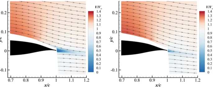
3.47 Wake velocity profile from PIV data forM= 0.7 andα=0◦at different chordwise locations. 66 3.48 Contour of wake velocity difference between suction and no-suction cases normalized by freestream velocity forM= 0.7 andα=0◦. . . 66

3.49 Airfoil-surface flow visualization for no-suction condition atM= 0.7 andα=2◦. . . 67

3.52 Airfoil-surface flow visualization for no-suction condition atM= 0.7 andα= -1◦. . . 68

3.53 Airfoil-surface flow visualization for no-suction condition atM= 0.7 andα= -2◦. . . 68

3.54 Airfoil-surface flow visualization for suction condition atM= 0.7 andα=2◦. . . 69

3.57 Airfoil-surface flow visualization for suction condition atM= 0.7 andα= -1◦. . . 70

3.58 Airfoil-surface flow visualization for suction condition atM= 0.7 andα= -2◦. . . 70

3.59 Averaged shock locations for each angle of attack, where “S” legend entries indicate suction. 71 3.60 Instantaneous Schlieren images of shock wave oscillation at α= 0◦ and M = 0.7 for no-suction case. . . 72

3.61 Instantaneous Schlieren images of shock wave oscillation atα=0◦andM= 0.7 for suction case. . . 72

3.62 Entire resolved power spectral density of shock oscillation atM= 0.7 andα=0◦for both suction and no-suction cases. . . 73

3.63 Power spectral density of shock oscillation up to 300 Hz forM= 0.7 andα=2◦no-suction case. . . 73 3.64 Power spectral density of shock oscillation up to 300 Hz forM= 0.7 andα=2◦suction case. 73

(11)

3.65 Power spectral density of shock oscillation up to 300 Hz forM= 0.7 andα=1◦no-suction case. . . 74 3.66 Power spectral density of shock oscillation up to 300 Hz forM= 0.7 andα=1◦suction case. 74 3.67 Power spectral density of shock oscillation up to 300 Hz forM= 0.7 andα=0◦no-suction

case. . . 74 3.68 Power spectral density of shock oscillation up to 300 Hz forM= 0.7 andα=0◦suction case. 74 3.69 Power spectral density of shock oscillation up to 300 Hz forM= 0.7 andα= -1◦no-suction

case. . . 75 3.70 Power spectral density of shock oscillation up to 300 Hz forM= 0.7 andα= -1◦suction case. 75 3.71 Power spectral density of shock oscillation up to 300 Hz forM= 0.7 andα= -2◦no-suction

case. . . 75 3.72 Power spectral density of shock oscillation up to 300 Hz forM= 0.7 andα= -2◦suction case. 75

(12)

Nomenclature

a speed of sound

A airfoil cross-sectional area nondimensionalized byc2

b0 airfoil semispan

B₁ first Bernoulli polynomial

B₂ second Bernoulli polynomial

c chord length

Ca airfoil axial force coefficient

Cd airfoil drag coefficient

Cdw wake drag coefficient

Cd0 drag coefficient parameter at each wake survey location

Cdm a x

0 _{maximum value of}

Cd0

Cf,l skin friction coefficient across the lower surface

C_f,u skin friction coefficient across the upper surface

C_l airfoil lift coefficient

Cm airfoil quarter-chord pitching moment coefficient

CmL E airfoil leading-edge pitching moment coefficient

Cn airfoil normal force coefficient

Cp airfoil pressure coefficient

Cp,cr it critical pressure coefficient

Cp,l airfoil pressure coefficient across the lower surface

C_p_,_u airfoil pressure coefficient across the upper surface

Cµ suction momentum coefficient

(13)

F acquisition rate

G spectral density function

h wind tunnel test section height

H sidewall boundary-layer shape factor

I pixel intensity

L/D lift-to-drag ratio

M Mach number

Mcr it critical Mach number

M∞ freestream Mach number

M∞c corrected Mach number

n number of measured quantities in parameter calculation

NS number of samples

Nens number of realizations for ensemble average

p general parameter calculated

P static pressure

P₁ static pressure at a survey location behind the wake P∞ static pressure at freestream conditions

P0 stagnation pressure

P0,1 stagnation pressure at a survey location behind the wake

P0,∞ stagnation pressure at freestream conditions

P∗ porosity parameter

q∞ freestream dynamic pressure

R ideal gas constant

Re Reynolds number

Re_x Reynolds number at correspondingxlocation S constant dependent onµ0in Sutherland’s law

S raw signal

Sens extracted raw signal from number of realizations

(14)

T period

T0 stagnation temperature

T1∗ total temperature in Sutherland’s law

T0∗ reference total temperature in Sutherland’s law

T∗ variable in Bernoulli polynomials

t/c airfoil thickness-to-chord ratio

t/c_max maximum airfoil thickness-to-chord ratio

u xcomponent of velocity uW velocity correction U uncertainty v ycomponent of velocity vW incidence correction V∞ freestream velocity

V/V∞ local velocity-to-freestream velocity ratio

V_s/V∞ suction velocity-to-freestream velocity ratio

x chordwise/streamwise direction

X discrete Fourier transform

x/c airfoil streamwise location-to-chord ratio

y chord-normal/freestream-normal direction

yw wake-parallel direction

Greek Symbols

α angle of attack

β Prandtl-Glauert compressibility correction factor

δ Pitot-static probe thickness

δ0 upwash factor

δ1 streamline factor

δ∗ _{sidewall boundary-layer displacement thickness}

(15)

∆M∞ Mach number correction

∆V/V∞ nondimensional velocity difference between suction and no-suction conditions

∆α angle-of-attack correction

S solid blockage factor

W wake blockage factor

γ ratio of specific heats

µ doublet strength in thexdirection

µ0 dynamic viscosity at of air at reference conditions

µair dynamic viscosity of air

ω doublet strength in theydirection

ΩS solid blockage ratio

ΩW wake blockage ratio

ρ∞ freestream air density

σ source strength

τ correction parameter dependent onP∗andβ

θ boundary-layer momentum thickness

Acronyms

DBD dielectric barrier discharge

DFT discrete Fourier transform

FFT fast Fourier transform

HALE high altitude long endurance

ISR intelligence, surveying, and reconnaissance

LPM liters per minute

NASA National Aeronautics and Space Administration

NLF natural laminar flow

OAR open-area ratio

PIV particle image velocimetry

(16)

RAE Royal Aircraft Establishment

SLA stereolithography

SNLF slotted natural laminar flow

UIUC University of Illinois at Urbana-Champaign

(17)

Chapter 1

Introduction

With aerodynamic efficiency and ecological concerns continuing to serve as driving parameters in new aircraft designs, the use of innovative technologies and design approaches to address present aerodynamic challenges such as drag reduction is paramount. Particularly to flight in the transonic regime, reducing skin friction drag is of high importance as, while being highly dependent on airfoil geometry it is also predominant at higher flight velocities. For transport aircraft, the wing profile drag has been estimated to be one of the largest contributors to drag, accounting for one third of the total drag at cruise conditions [1, 2]. The application of laminar flow airfoils to these types of aircraft could potentially offer a way to reduce the skin friction drag by extending the laminar flow region of the airfoil boundary layer further aft than current transonic airfoil designs [3, 4]. In fact, at the airplane level, the net drag reduction benefits of laminar flow control have been estimated through NASA-supported studies to be as high as 10% [5].

In addition to commercial transport aircraft, there is another category of aircraft that operates in the transonic regime that could benefit from aerodynamic performance improvements resulting from laminar flow. This class of aircraft, known as High-Altitude, Long-Endurance (HALE), are commonly used for intelligence, surveying, and reconnaissance (ISR), communications relaying, weather and agricultural mon-itoring, and other applications requiring satellite-based systems [6–11]. Generally, these aircraft are de-signed to operate for long periods of times at target altitudes of up to 35 km [12]. For example, the Global Hawk used by the U.S. Air Force for ISR has a service ceiling of 60,000 ft. and endurance of more than 34 hours. Hence, this high-altitude operating requirement presents an unconventional application outlined by low Reynolds number and transonic Mach number conditions. As a result, these aircraft are also character-ized by lower wing loadings (larger surface area), which poses a need for highly efficient airfoil sections in order to minimize the viscous drag component and increase aerodynamic efficiency.

It is evident that aircraft operating in the transonic regime can benefit from the improvements in aero-dynamic efficiency that are provided by laminar flow technology. This introduces an alternative way of

(18)

increasing aircraft efficiency from an aerodynamic design perspective, rather than by just improving power plant efficiency as is recently been done. However, laminar-flow airfoils have generally been designed for low-speed and low-Reynolds number applications as these conditions allow for better control and tailoring of the boundary-layer transition process. Flight in the transonic regime introduces challenging influences that promote transition, such as shock waves and cross flow under swept wings, for example, that limit the ability to retain laminar flow. Therefore, different design considerations using different methods of flow control (instead of the conventional natural-laminar-flow approaches used for low speeds) should be consid-ered for transonic, laminar-flow airfoils. This investigation intends to indentify the laminar flow capabilities, aerodynamic performance gains, and transonic characteristics of a laminar-flow airfoil concept using active flow control through boundary-layer suction.

1.1 Laminar Flow Technology and Challenges in a Transonic Flow Field

The idea of natural-laminar-flow (NLF) airfoils has been widely studied for low-speed configurations and recently has gained interest for applications to transonic aircraft [1, 2, 13, 14]. However, studies have shown that the implementation of an NLF transonic wing poses a substantial challenge for conventional commercial transport aircraft due to the associated high leading edge sweep angles and high operating Reynolds numbers [15]. Historically, the application of NLF airfoils has been constrained to low sweep, low-Reynolds number conditions, as both of these parameters have a direct influence on the growth of modal instabilities, such as the natural growth of Tollmien-Schlichting (T-S) waves and cross-flow modes that promote early transition [3, 4]. However, there have been attempts to achieve NLF at transonic conditions with limited success.

An example of an NLF transonic airfoil was the HSNLF(1)-0213 designed to operate at M= 0.7,Cl =

0.25, andRe= 11 x106[16]. The application of this airfoil was intended for a single engine business jet with no sweep. The constraint on the sweep already poses a limitation on the maximum achievable Mach number of an aircraft due to the inability of NLF designs to sustain laminar flow under cross-flow instabilities. Due to compressibility effects, at higherCl values the flow across the upper surface of the airfoil continues to

accelerate, increasing the extent of the favorable pressure gradient region rather than achieving high suction peaks near the leading edge as is common in an incompressible-flow condition. It was found during the development of the airfoil that this favorable pressure gradient region which terminated in a shock led to a steep aft pressure recovery which was very susceptible to separation. The final geometry was tailored for a

(19)

shock-free design with favorable pressure gradients extending to 55%con the upper surface and 65%c on the lower surface. Also, the turbulent pressure recovery across the upper surface of the airfoil was optimized to prevent separation [16]. Even though this case study demonstrates the capabilities of obtaining laminar flow at very high speeds, it does not technically qualify as a transonic application since the final geometry was tailored to not have shocks and therefore no local supersonic region.

Another concept that has recently been studied is the slotted, natural-laminar-flow airfoil (SNLF) [1, 2, 13, 14]. The SNLF concept involves a two-element airfoil which is able to extend the laminar flow capabilities beyond the limits of current airfoils. By introducing an aft element, the pressure is no longer required to recover to freestream conditions at the trailing edge of the fore element, allowing the favorable pressure gradient to be extended across a significantly larger portion of the chord. In addition, since the wake of the fore element does not impinge on the aft element, laminar flow across this smaller aft element of the airfoil could also be achieved [13]. The aft element is then responsible for recovering the pressure over a shorter distance as momentum is added to the boundary layer through the slot, allowing the boundary layer to sustain a larger recovery pressure gradient without separating. The concept shows potential to significantly increase the extent of laminar flow regions when compared to conventional airfoil designs, experimentally shown to be transition free at low-Reynolds number and low-speed conditions at a notable angle-of-attack range [13]. However, the airfoil’s ability to retain laminar flow under moderate sweep, at off-design conditions, at higher Reynolds numbers, and in the presence of transonic shocks across the surface of the airfoil should be considered. Additionally, special treatment should be given to the design of the slot considering the possibility of choking at higher transonic Mach numbers.

Laminar-flow airfoils with active boundary-layer control could potentially be used as an alternative to natural-laminar-flow approaches. These airfoils are designed with some form of actuation to actively control the boundary layer, extending the region of laminar flow across the surface. For example, active transition control can be performed through means of pressure gradient control, mean wall-temperature control, wall suction, and recently by using dielectric barrier discharge (DBD) plasma actuators. These approaches inhibit the growth of T-S waves, and in some cases crossflow instabilities, in order to prevent or delay boundary-layer transition [17–19]. The application of Griffith’s airfoil concept, which uses active boundary-layer control through suction, is explored in this study as a method of achieving laminar flow in transonic conditions.

(20)

1.2 Griffith’s Laminar-Flow Airfoil Concept

The concept of suction-enabled laminar flow airfoils was first introduced by Griffith in the early 1940’s [20, 21]. Griffith’s airfoil was designed to have a favorable pressure gradient across most of the upper surface. However, as the streamwise portion of the airfoil designed with a favorable pressure gradient region is increased, the pressure must recover across shorter distances and stronger adverse pressure gradients which may lead to detrimental characteristics such as boundary-layer separation. To overcome the performance penalties associated with such traits, the pressure recovery was aided through a suction slot located near the airfoil trailing edge. Given that the suction system allowed the pressure to be recovered to freestream values across short distances without separating, the airfoil experienced extensive laminar flow runs across the upper surface as a result of the extended favorable pressure gradient region dictated by the airfoil geometry. This feature resulted in significant skin friction drag reductions relative to conventional airfoil designs at the time [21].

Similar design methods were also used by Goldschmied [22]. One of his most noteworthy designs was the thick-wing spanloader which incorporated a centrifugal blower to provide boundary-layer suction. This approach enabled a Griffith-type, laminar-flow airfoil concept to be used, where the blower exhaust was then routed out the trailing edge of the airfoil [22]. This mass ejection out of the trailing edge in the design provided an extra source of thrust, which also contributed to offsetting the skin friction drag component of the airfoil.

It has been shown through many studies that large lift coefficients and drag performance benefits can be obtained from these types of suction-enabled airfoils [23]; however, as previously mentioned laminar-flow airfoils have typically been designed for low speeds, making them incompatible for transonic applications. For example, Griffith’s airfoilt/cof 0.30 limits its Mcr it to a very low value, leading to significant

com-pressibility losses at transonic Mach numbers of transport-class aircraft. In the case of HALE aircraft which have larger t/c to achieve lofty Cl requirements, consideration should be given to the tradeoff between

compressibility losses and the effects of laminar separation bubbles which are typical at their low-operating Reynolds numbers. Nevertheless, the use of Griffith’s pressure recovery across a limited region assisted by suction upstream of the trailing edge can be implemented in the design of laminar-flow airfoils for transonic applications.

(21)

1.3 Research Motivation

As new and improved aircraft designs are developed, it can be seen that focus has been given to engine efficiency, lowering fossil-fuel consumption, and reducing the emission-based carbon footprint of aviation. These considerations are all targeted to the power generating aspect of the aircraft that produces the required thrust to sustain flight. With the exception of a number of new clean-sheet aircraft designs, little importance has been given to improving the efficiency of an aircraft from an aerodynamic design perspective as new aircraft being developed are mostly based from existing designs with modifications that only improve engine efficiency and add novel capabilities. Therefore, innovative aerodynamic concepts that push the limits of existing performance boundaries should be implemented in the development of next generation aircraft. In particular, laminar-flow technology should be considered for transonic wing designs as skin friction drag is a major contributor of the overall drag of an aircraft at high speeds. This technology displays the ability to provide substantial reductions in drag increasing the aerodynamic efficiency of wings, which in turn will lead to reduced fuel consumption. However, to develop adequate wing concepts able to significantly increase current laminar flow capabilities in a transonic flow field, there first needs to be suitable airfoil designs capable of achieving and maintaining laminar flow in the same flow conditions. This initially requires extensive wind tunnel testing to evaluate airfoil performance and identify characteristics not captured in simulations to facilitate further advancement of airfoil concepts.

1.4 Research Objectives

The purpose of this investigation is to assess the ability of Griffith’s airfoil concept to provide laminar flow and improve aerodynamic efficiency in a transonic flow field. For this study a transonic, laminar-flow airfoil developed by Perry et al. [21] and Kerho et al. [24] using Griffith’s method of suction for pressure recovery was used. The the magnitude of increased aerodynamic efficiency that can be obtained from this airfoil is considered by comparing its performance to that of the same geometry without suction applied as well as to another transonic airfoil. In addition, the study aims to identify important characteristics of the airfoil that are relevant to operation in a transonic flow field. This approach could be used to further improve the airfoil design considering tradeoffs between aerodynamic benefits obtained and compressibility losses in the transonic regime. These goals were attained through the collection of pressure data that allowed

(22)

the aerodynamic performance of the airfoil to be characterized, as well as the use of other experimental diagnostics tools such as PIV, surface-oil flow visualization, and Schlieren imaging to identify relevant wake effects, transitions characteristics, and shock behavior. In general, the specific objectives of the experimental investigation on the Griffith-type transonic, laminar-flow airfoil are outlined as follows:

• Understand the boundary-layer suction influence on theCp distributions of the airfoil and the effect

on the pressure recovery

• Characterize the aerodynamic performance across a range of angles of attack and Mach numbers as well as determine the magnitude of profile drag reduction and improved lift-to-drag performance that can be achieved

• Analyze the influence in the laminar flow capabilities and transition characteristics of the airfoil under the influence of boundary-layer suction

• Identify the effect of suction on the development, stability, and strength of the resultant transonic shock across the upper surface of the airfoil

(23)

Chapter 2

Experimental Methodology

This chapter introduces the different methods and experimental techniques used during the investigation performed at the University of Illinois at Urbana-Champaign (UIUC). Detailed descriptions of the test fa-cility, data acquisition equipment and execution, calculation of aerodynamic parameters, and test setup and configurations are provided within.

2.1 Transonic Wind Tunnel Experimental Facility

The experimental campaign for this investigation was conducted in the newly-developed Transonic Wind Tunnel Facility at UIUC. The test facility is housed in the dedicated laboratory room 131 in the Aerodynam-ics Research Laboratory. This transonic wind tunnel is a suction-type, open-return wind tunnel featuring a test section with a cross-sectional area measuring 6” by 9” and running 18” in the streamwise direction. Figure 2.1 shows the transonic wind tunnel used.

In order to condition the flow going into the test section, the tunnel houses a settling chamber in the inlet section with an initial layer of honeycomb followed by three layers of turbulence-reducing screens. Essentially, the honeycomb acts as a flow straightener initially reducing large-scale turbulence associated with swirling of the flow during entry, while the subsequent screens reduce the overall turbulence intensity of the flow (some of which is generated by shear layer instabilities and Reynolds stresses associated with the honeycomb) improving angularity and velocity uniformity [25–28]. The ratio between the inlet and test section of the tunnel is 27.88. This configuration resulted in turbulence intensities of less than 0.04% at all Mach number conditions determined through Particle Image Velocimetry (PIV) experimentation.

In transonic wind tunnel testing, porous or slotted test-section wall bondaries are generally incorporated in test sections to help mitigate compressibility effects such as shock reflections from the walls and artificial curvature of streamlines at high dynamic pressures [29]. Consequently, this wind tunnel was designed with

(24)

6% open-area ratio top and bottom walls with 0.25” thickness and a hole diameter-to-thickness ratio of 1. The holes were also machined at an angle of60◦relative to the surface. This feature allows a desired pressure difference between the test section and plenum chamber to be achieved with a lower open-area ratio. In turn, it also helps the flow from reentering into the test section when the pressure in the plenum chamber is higher than that of the test section due to the extra pressure head the flow must overcome [29]. Both upper and lower sides of the porous test section have a 2” plenum chamber that serves as a bypass region to the flow coming out of the test section. The pressure in this plenum can be controlled to some extent using suction flaps located downstream of the test section, which control the amount of air that exits the plenum into the diffuser. Initially, a sensitivity study was performed to verify the influence of the suction flap locations. It was observed that after some small extent of the flap opening, no further significant change was observed in theC_pdistribution of the model. Furthermore, setting them fully open did not have a detrimental effect on the wind tunnel performance. For these reasons, the plenum flaps were set at90◦ relative to the wall orientation throughout this investigation. The top porous wall and plenum were also fitted with a 6.0”× 0.07874” slot to allow for the passage of a laser sheet in order to perform PIV experiments.

The test section was also fitted with removable sidewalls in order to install and remove airfoil models. These walls were designed with an acrylic insert of 9.30”×7.15”. The set of windows provided a means to observe the aerodynamic model during testing for any abnormalities as well as allowed for optical ac-cess required in certain experimental techniques. The acrylic inserts were drilled with holes for support spars to pass through at a 5” location in the streamwise direction and at a half test-section height location. This approached allowed for the installation of aerodynamic models with spars having a diameter of up to approximately 0.5”. The left spar of the models installed was passed through an Accu-CoderProTM Pro-grammable Incremental Encoder Model 58TP manufactured by Encoder Products Company with a rated accuracy of±0.015◦ from true position. This encoder has a 0.5” thru-bore fitting which was fixed to the shaft of the model to track the angle-of-attack position. The encoder was programmed with 36,000 counts per revolution, which provided a resolution of0.01◦. The encoder index location (which indicated the0◦ angle-of-attack position) was also programmed during the installation using a stencil of the airfoil alongside a level. The angle-of-attack readings were then observed and recorded using a US DigitalR ED3 Digital

Encoder Display which converted the differential quadrature signals into degree measurements through an internal firmware.

(25)

Once fitted through the encoder, the model was connected through a shaft-coupling linkage mechanism to an Anaheim Autonation 34 MDSI214S stepper motor. This stepper motor had a 1,200 oz-in maximum holding torque and a 0.225◦ resolution using microsteps. The same stepper motor model was used for control of the suction plenum flaps in the plenum chamber.

The wind tunnel was powered via an ABB ACS880 variable frequency drive (VFD). This VFD was used to control the power to a Baldor-Reliance 255 HP motor which was responsible for driving the AirPro model 420 centrifugal blower at the diffuser end of the wind tunnel. The reason this tunnel is operated via a centrifugal blower rather than a conventional fan is because a centrifugal blower is able to accommodate larger pressure losses inside of the test section which are inherent to transonic conditions. The maximum motor operating setting of approximately 2,120 RPM resulted in a maximum Mach number of 0.85 for an empty test section. However, when an experimental airfoil model with chord of 6” is introduced, the maximum Mach number reached is approximately 0.725. The maximum Mach number also varied with variations in angle of attack as the blockage introduced by the model changed.

The operating Mach number and freestream velocity were determined based on the stagnation pressure, static pressure in the test section, and ambient temperature in the laboratory. The pressures were measured using two OMEGAR PX409-030A5V-EH pressure transducers which had a rated accuracy of±0.05%. The stagnation pressure measurement was taken downstream of the settling chamber where the flow velocity was considered to be negligible compared to that in the test section; hence, the static pressure measured was assumed to be same as the stagnation pressure in this region. The static pressure measurement under a non-zero dynamic pressure was taken through a pressure tap located in the upstream end of the test section ceiling. The freestream Mach number (M∞) was then calculated using the following isentropic relationship:

P P0 = 1 +γ−1 2 M∞ 2 _γ-₋γ₁ (2.1) wherePis the static pressure,P0is the stagnation pressure, andγ is the ratio of specific heats.

In order to also determine the actual freestream velocity in the test section, stagnation temperature measurements of the laboratory conditions were taken using a National Instruments USB-TC01 J-type ther-mocouple. The static temperature was then calculated using the following relationship:

P P0 = T T0 _γ-₋γ₁ (2.2)

(26)

whereT is the static temperature andT0is the stagnation temperature.

Using the static temperature calculated for the test section, the speed of sound (a) and freestream velocity (V∞) were calculated using:

a=pγRT (2.3)

V∞ =M∞a (2.4)

whereRis the ideal gas constant.

2.2 Airfoil Models

2.2.1 Griffith-Type Transonic, Laminar-Flow Airfoil

The airfoil used for this experimental investigation was the Griffith-type transonic, laminar-flow airfoil developed by Perry et al. [21] and Kerho et al. [24] for application in a commercial-transport aircraft. An in-depth analysis of the development of the airfoil can be found in References [21] and [24]; however, a general overview of the design criteria and resulting airfoil characteristics are discussed.

The objective of the Griffith airfoil is to achieve extensive regions of laminar flow across the airfoil surface. This is done by tailoring the airfoil geometry to have regions of favorable pressure gradient across most of the upper surface which promote laminar flow. The pressure is then recovered rapidly across a short recovery region by means of boundary-layer suction through a slot located near the trailing edge, which helps maintain attached flow in the presence of a strong adverse pressure gradient [20]. Early experimental work from Richards et al. [20] at low-Reynolds numbers and low-subsonic conditions demonstrated that an effective suction location for such an airfoil concept was located near the trailing edge pressure recovery region, around x/c= 0.70. The effect of the slot width and mass flow suction was also part of the afore-mentioned investigation [20]. It was found that the proportion of the boundary-layer volume removed did not increase when varying the slot width size in the chordwise direction for a fixed suction amplitude for slot widths greater than approximately 70% of the boundary-layer thickness. In a similar way, the required proportion of the boundary-layer volume that had to be removed in order to prevent separation did not

(27)

in-crease as the slot width was inin-creased up to the thickness of the boundary layer at the suction chordwise location [20].

In order to design a transonic, laminar-flow airfoil incorporating the Griffith concept, a number of de-sign constraints were set considering desired performance objectives. Commercial aircraft that operate at transonic speeds have airfoil thicknesses that typically range fromt/_c _{of 9%-12%. In order to produce a}

reasonable Mcr it for the candidate airfoil, a design constraint oft/cmax = 15% was set. The design Mach

number was set to 0.7, also representative of operational speeds of airfoil sections for modern commer-cial and business aircraft. While this operational Mach number is lower than the vehicle cruise speed used in modern transonic air transport vehicles, this design condition could be utilized with a limited extent of sweep to mitigate adverse compressibility effects at higher vehicle cruise Mach numbers.

An inverse airfoil design code, Profoil, was used to generate the airfoil geometry based on desiredC_p distribution characteristics of a nominal flow airfoil. An example of a notional, transonic laminar-flowCp distribution is presented in Fig. 2.2, after Cella et al. [30] at three different flight configurations.

Validation of the designed airfoil shape was performed using OVERFLOW CFD to obtain predictions of the airfoil performance which are included in Reference [21]. The final airfoil presented by Perry et al. [21] and Kerho et al. [24] has at/_c _{of 12.48% and was designed to produce extensive laminar flow at a freestream}

Mach number of 0.7 and angle of attack of0◦. Transition across the upper and lower surfaces was predicted to occur at 0.57cand 0.45c, respectively, at the design Reof 16.2 million. The suction slot has a location between 0.825c and 0.875c, with a design suctionVs/V∞ = 6.5% orCµ= 0.00014 [21, 24]. A rendering of

the transonic airfoil design is presented in Fig. 2.3.

A small-scale model of this airfoil was designed and built in order to measure its aerodynamic per-formance at the full-scale Mach number and a transitional Reynolds number range. The chord and span were selected to be 6”, allowing the airfoil to occupy the entire test section in the spanwise direction when mounted horizontally to help mitigate three-dimensional effects during testing. An array of 41 pressure taps with outer diameter of 0.045” were incorporated into the model and routed internally through the left spar of the model to obtain static pressure measurements across the upper and lower surfaces of the airfoil. The taps were manufactured with a 12◦ sweep angle in the streamwise direction to reduce the influence of disturbances and possible boundary-layer transition induced by upstream pressure taps in the acquired measurements. The model was designed in a two piece assembly, such that the internal cavity served as a

(28)

suction plenum with an opening at the desired suction location on the airfoil. Originally, the leading edge portion of the airfoil model was manufactured from polished aluminum while the trailing edge portion was 3D printed using stereolithography (SLA). The SLA trailing-edge part featured internally routed pressure taps and was only used during the acquisition of the surface pressure data and for PIV experiments. An identical trailing-edge piece constructed of polished aluminum was substituted when wake pressure data were taken and when performing Schlieren experiments. The main body of the model consisting of the leading-edge and trailing-edge parts described spanned 5.2”. Two aluminum side plates, having the same airfoil geometry and thickness of 0.25”, were fastened to the main body to serve as an interface with the spar support. Lastly, two TeflonR covers also with the same airfoil geometry and thickness of 0.15” were

fixed to each side to avoid scratching between the experimental model and the sidewall.

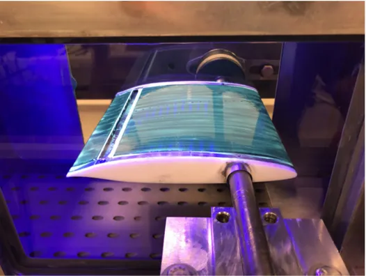
In order to provide suction to the airfoil, a pneumatic shaft was attached to the right side of the model. This shaft also served as a structural spar to support the model at the quarter-chord point. The suction slot was fitted with interchangeable cover plates, one with the 0.05cslot open area across the span and the other completely covered to allow for testing of the baseline airfoil without any suction applied. Due to size constraints and experimental limitations, mass ejection out the trailing edge could not be implemented in the experimental model as was used by Goldschmied [22] and also considered in the development of the original airfoil design [21, 24]. A photograph of the experimental model is presented in Fig. 2.4, mounted inside the test section of the wind tunnel.

Suction to the airfoil model was applied across the slot on the airfoil by means of a Venturi suction pump, which was connected through pneumatic lines at the end of the pipe internally routed to the suction plenum inside of the model. The Venturi pump used was a VACCON Model VDF750-ST16C. The pneumatic line from the suction pump was routed through a mass flow meter in order to record the suction being applied at the slot during different test configurations. For this an Alicat Scientific M-Series Model M-3000SLPM-D/5M mass flow meter configured for air was used having a rated accuracy of±0.8% of the measurement reading. The varied suction requirements through the different test configurations were controlled through a pressure regulator located prior to the air supply of the Venturi pump.

(29)

2.2.2 RAE 2822 Transonic Airfoil

In order to directly compare the performance benefit of the boundary-layer, suction-enabled design of the Griffith-type airfoil, aerodynamic data from other airfoil geometries designed to operate in the same regime are beneficial. Furthermore, due to the inherent limitations of the transonic test facility, data for transonic airfoils at the low Reynolds numbers achieved during experimental runs are hard to obtain. For this, an RAE 2822 model was fabricated and tested at the same flow conditions in order to provide a means of comparison. The RAE 2822 airfoil, developed by the Royal Aircraft Establishment, was selected for its well-known transonic characteristics. This airfoil is also frequently used as a canonical case for numerical and experi-mental studies, as well as for CFD validation. In addition, there are historical data at similar low Reynolds number conditions (2.7 million) to those achievable in the transonic test facility, providing an additional source of validation for the RAE 2822 data and ensuring reliability of the acquired measurements. There-fore, it was fitting to select this model as a basis of comparison.

The original geometry of the RAE 2822 has a sharp trailing edge which poses difficulties in its manu-facturing and internal pressure tap routing. A modification to the original RAE 2822 airfoil geometry was used to incorporate a discrete-finite trailing edge. This modification was performed using XFOIL’s built-in function TGAP. This function allows the user to define the gap between upper and lower surfaces of the trailing edge along with a blending distance defined from the leading edge which controls the degree of blending between the newly-defined trailing edge to the original airfoil geometry [31]. For the modified RAE 2822 geometry, a trailing-edge gap thickness of 0.066” was set alongside a blending distance of 0.25c. The resultant geometry can be seen in Fig. 2.5.

An experimental model was built using the modified RAE 2822 airfoil with the same chord and span lengths of 6”, resulting in an aspect ratio of 1. The span extending the width of the test section limited three-dimensional influences that would be caused at the tips of the model, while the 6” chord ensured that the same chordwise Reynolds numbers would be achieved at the different Mach numbers being tested. Similarly to the Griffith experimental model, the main body of the airfoil extended 5.2” inches in span. Two sideplates with the same airfoil geometry, each with a width of 0.25”, were fastened to both sides of the main body to interface with the structural supports. Two shafts with 0.5” diameter were welded to the sideplates at the quarter-chord location of the airfoil. These shafts served as structural spars to appropriately set the angle-of-attack conditions as well as support the model during testing. Additionally, two TeflonR covers

(30)

with the same airfoil geometry and thickness of 0.15” were fixed to the ends of the sideplates to avoid any possible scratching on the sidewalls. This design having the main airfoil body as a single shell facilitated the installation of internal pressure taps. Similarly, an array of 40 pressure taps were incorporated along the upper and lower surfaces of the airfoil. These taps were used to record static pressure measurements that would then be utilized to calculate integral aerodynamic coefficients of lift and moment. The taps were also manufactured with a12◦sweep angle in the streamwise direction. This feature helped to ensure that the boundary-layer region over a pressure tap would not be artificially contaminated (transitioned) by the influence of upstream taps. The RAE 2822 experimental airfoil model can be seen mounted inside the wind tunnel in Fig. 2.6.

2.3 Aerodynamic Wind Tunnel Tests

To characterize the aerodynamic performance of the airfoils being tested, integral aerodynamic coefficients were calculated using a combination of airfoil-surface pressure measurements as well as wake pressure measurements. The following subsections outline the data acquisition and calculation processes as well as the wind tunnel corrections applied.

2.3.1 Airfoil-Surface Pressure Measurements

Airfoil-static pressure measurements were taken through the pressure taps internally routed through the air-foil model as previously described in Sections 2.2.1 and 2.2.2. The metal tubing of the pressure taps, which were accessed through the left spar of the model outside of the test section, were connected via polyurethane tubing with inner diameter of 0.045” to interface with the pressure measurement system. The pressure read-ings for the Griffith airfoil-surface pressures as well as all wake pressures (for both airfoil models) were acquired using a Pressure Systems Incorporated (PSI) NetScanner Pneumatic Intelligent Pressure Scanner system, Model 9116. A new DTC Initium Data Acquisition System with a PSI 64-channel 15 PSID ESP Miniature Pressure Scanner system was also acquired and used for the surface pressure measurements of the RAE 2822. However, both systems were manufactured by the same supplier and had the same basic performance and precision characteristics mostly differing by the number of available channels.

The PSI NetScanner system featured 16 channels, 12 of which were rated at 15 PSID. These channels were the only ones used to ensure the best resolution in the data. The rated accuracy of the system was

(31)

given to be±0.05% of the full-scale reading. The system also had a supply port incorporated for inert gas in order to provide pressure when operating an internal valve mechanism for calibration of the pressure ports. For this, high-purity nitrogen was used and supplied at a pressure of 100 PSI as recommended by the manufacturer. The system was recalibrated before each experimental run. Since the individual pressure transducers measure a pressure differential relative to a reference value, the system has a dedicated port for a reference pressure to be supplied which was referenced by each of the individual transducer channels. During testing, this reference pressure port was connected to the freestream static pressure in the test section. This allowed the difference between the local surface pressure and the freestream conditions to be directly measured, making it easier to directly compute local Cp values. The pressure data were acquired at a

sampling rate of 30 Hz for 10 seconds and subsequently averaged for each test case.

The PSI 64-channel 15 PSID Miniature ESP Pressure Scanner system coupled with the DTC Initium Data Acquisition system worked in a similar way, varying mostly in the additional total number of channels that could be sampled at a given time. The accuracy rating was also ±0.05% of the full scale reading. Similarly, the system was calibrated by supplying nitrogen at 100 PSI, and the pressure differential was based on a reference pressure port which was connected to the freestream static pressure. Sampling was performed at a frequency of 50 Hz for 5 seconds for which data were then averaged.

Pressure Coefficient Calculation

In order to calculate the pressure coefficient distribution about the airfoil, the freestream dynamic pressure had to be determined. Since operating in the transonic regime where incompressible assumptions do not hold and no direct measurement of the freestream density in the test condition was available, the dynamic pressure was determined by subtracting the stagnation pressure and test-section static pressure measurements using the pressure transducers described in Section 2.1. Equation 2.5 shows the calculation for dynamic pressure which was performed through the data acquisition software described in Section 2.3.3. In Eq. 2.5,P0is the

stagnation pressure andPis the static pressure, both assumed to be at freestream or test-section conditions.

q∞ =P0−P (2.5)

(32)

C_p = P−P∞ q∞

(2.6) where P−P∞ is the difference between the surface-static pressure at a particular airfoil location and the

freestream static pressure. This value was directly recorded which allowed theCp values to be calculated

and recorded through the data acquisition program.

Lift and Moment Coefficients Calculation

The two-dimensional lift and moment coefficients were obtained by integrating the pressure distributions obtained from the airfoil. It is known that all aerodynamic forces and moments produced on an airfoil shape result from pressure and shear-stress distributions. Hence, the following expressions for the normal force (perpendicular to the chordline), the axial force (parallel to the chordline), and the moment about the leading edge can be derived for an airfoil only considering pressure and shear stress in nondimensional coefficient form as follows: cn= 1 c Zc 0 Cp,l−Cp,u dx+ Zc 0 Cf,u dyu dx +Cf,l dyl dx dx (2.7) ca = 1 c Zc 0 Cp,u dyu dx −Cp,l dyl dx dx+ Zc 0 Cf,u+Cf,ldx (2.8) (2.9) cmL E = 1 c2 Zc 0 Cp,u−Cp,lxdx− Zc 0 Cf,u dyu dx +Cf,l dyl dx xdx + Zc 0 Cp,u dyu dx +Cf,u yudx+ Zc 0 −Cp,l dyl dx +Cf,l yldx

where the subscripts u andl indicate upper and lower surfaces of the airfoil respectively, C_f is the skin friction coefficient, and dy_dx is the local slope of the airfoil surface. As can be seen from Eqns. 2.7 and 2.8, it can be noticed that the contribution of the skin friction component acts primarily on the axial component of the force and has a negligible effect on the normal component as it is being multiplied by the local airfoil slope which is generally very small. Since the lift coefficient (Eq. 2.13) depends primarily on the normal component of the force, particularly at low angles of attack which happens to be the case in this investigation, the skin friction terms can be ignored and the coefficients become:

(33)

C_n = 1 c Zc 0 C_p,l−Cp,u dx (2.10) Ca = 1 c Zc 0 Cp,u dyu dx −Cp,l dyl dx dx (2.11) C_m_{L E} = 1 c2 Zc 0 C_p,u−Cp,l xdx+ Zc 0 C_p,u dyu dx yudx− Zc 0 C_p,l dyl dx yldx (2.12) This assumption, however, does limit the parameters that we can obtain from surface-pressure data toCl

andCm, sinceCd is highly dependent on the axial component of the force.

The upper surface of the airfoil was fitted with 24 pressure taps and the lower surface with 17 pressure taps that were spanned across the chord at locations of interest. Therefore, to calculate the integral pa-rameters from Eqs. (2.10) to (2.12), the trapezoidal rule was implemented, where the mean pressure values between two adjacent pressure taps were assumed to define the pressure distributions across the upper and lower surfaces. The final coefficients were obtained by taking the difference between the upper and lower surface contributions as indicated by each respective equation.

With theCn,Ca, andCmL E, the lift and moment coefficients were calculated using the following rela-tionships:

Cl =cncos(α)−casin(α) (2.13)

Cm=CmL E + 1

4 Cl (2.14)

whereCl is the lift coefficient,αis the angle of attack, andCmis the moment coefficient about the

quarter-chord location.

2.3.2 Pitot-Static Wake Survey Traverse

As was discussed in Section 2.3.1, the drag generated by an airfoil is highly dependent on shear-stress influences that were neglected in the formulation of the axial force coefficient. Therefore, a pitot-static wake survey traverse was installed in the test section to capture the pressure deficits in the wake generated by the

(34)

airfoil under different test conditions. The wake survey traverse featured a single pitot-static probe with a single stagnation pressure orifice measuring 0.015”, four static pressure orifices measuring 0.0265”, and an external diameter of 0.125”. The probe was located at the center of the test section and 3.8” behind the airfoil model and was traversed vertically at 0.05” intervals using a ZABER Model T-LSR450B motorized linear traverse installed outside of the plenum chamber. Pressure data were obtained across a 2” region in order to ensure that the entirety of the wake was captured. This traversing region was determined during initial experimental runs where the stagnation pressure was observed to be constant and the wake tails could be identified. On average, the wake occupied a 0.5” linear region. The pressure measurements were obtained using the same PSI NetScanner system introduced in Section 2.3.1. Pressure data were taken for 5 seconds at a frequency of 30 Hz at each traverse location. An image of the pitot-static wake survey traverse system installed in the transonic wind tunnel can be seen in Fig. 2.7.

Drag Coefficient Calculation

Drag coefficients were obtained using the stagnation and pressure measurements obtained across the wake region using Betz’s method found in Reference [32]. This method is advantageous for the current study, as it allows for the survey to be performed at a location where the pressure and velocity have not yet recovered to freestream conditions, while taking into account compressibility effects. The method utilizes a momentum conservation approach for which the following relationship is obtained for each location along the wake:

Cd0= 2 P0,1 P0,∞ γ_γ−1 P1 P∞ _γ1            1− P1 P0,1 γ_γ−1 1− P∞ P0,∞ γ_γ−1            1 2          1−            1− P∞ P0,1 γ−_γ1 1− P∞ P0,∞ γ_γ−1            1 2         (2.15)

Once the distribution ofCd0values are calculated for each location surveyed in the wake region, they can

be integrated to obtain the two-dimensional drag coefficient (C_d) in the following way:

Cd=

Zyw

0

Cd0dy (2.16)

whereywis the height or length of the wake. Through the data obtained, total pressure losses were observed

particularly at higher Mach numbers as was expected due to compressibility effects. Hence, the difference between the stagnation pressure measurements obtained outside of the wake region were averaged and the

(35)

difference was found between the averaged freestream stagnation pressure recorded for the wind tunnel. This difference was then added to each total pressure value to offset the averaged total pressure loss. The integration was then performed from one wake-tail end to the other. The wake tails were determined by the point where the ratio between the local stagnation pressure and the freestream stagnation pressure decreased to a value lower than 1. Once the wake region was identified, the integration was performed using the trapezoidal rule at the midpoints between two adjacent data points.

2.3.3 Data Acquisition System

The data for the tunnel conditions, airfoil-static pressure measurements, and wake pressure measurements were taken using a custom software written in the National Instruments 2016 LabView programming en-vironment. This software was run on an HP Z230 Workstation with an IntelR XeonR CPU E3-1240 v3,

measuring clock speed of 3.4 GHz, 8 GB of RAM, and a Windows 10 Pro 64-bit operating system. This software provided the user with a graphical interface to calibrate, tare, or initialize different data acquisition components, and take data points individually or simultaneously.

Acquisition of experimental values was divided into three main components. The first component in-cluded acquisition of the general tunnel parameters including total, stagnation, and dynamic pressures, total and static temperatures, speed of sound, freestream velocity, and Mach number of the freestream flow recorded at a frequency of 2 Hz. The pressure values were obtained using the pressure transducers discussed in Section 2.1 interfaced with the software through a National Instruments NI USB-6009 Multifunction I/O Device using analog channels which was connected to the computer using a USB cable. The pressure transducers were properly calibrated based on curves provided by the manufacturer. The total temperature measurements obtained through the thermocouple, also described in Section 2.1, which interfaced directly with the software through a USB connection. The second data acquisition component consisted of the pres-sure meapres-surements. Two variants of the code existed depending on if data were taken for surface or wake pressure measurements. The devices used for obtaining these data values interfaced with the computer via an Ethernet connection using Protocol Version 4 (TCP/IPv4). Their operation and acquisition rates are dis-cussed in Section 2.3.1. The third acquisition component was the mass flow system for the suction cases of the Griffith airfoil. These data values were obtained via an RS-232 communication protocol between the mass flow meter and the computer using an RS-232-to-USB adapter. Volumetric flow rates were then

(36)

obtained at a frequency of 35 Hz. The software provided the option to record measurement sets individually or all together for surface-pressure and wake-pressure runs separately. When performing PIV, Schlieren, and flow visualization experiments, only tunnel conditions and mass flow (if necessary) data were obtained. In addition, the stepper motors discussed in Section 2.1 used to set the position of the suction plenum flaps and model angle of attack were controlled via this software. For this, an RS-232 communication protocol was used with the motors interfacing with the computer via an RS-232-to-USB adapter. The software allowed for their initialization when initially turned on to set the holding torque as well as to send position commands in degrees relative to their previous position. All commands to set specific angles in the suction flaps and the angle of attack of the airfoil model were executed before commencing operation of the wind tunnel during experimental runs.

2.3.4 Wind Tunnel Corrections

Test sections in wind tunnels are constrained by physical and finite boundaries which inherently prevent ab-solute atmospheric conditions to be replicated. Furthermore, the solid boundaries impose three-dimensional influences in the flow, which become more predominant when the test article’s aspect ratio is small. This influence poses a constraint when considering airfoils, since their performance is representative of a two-dimensional flow. In addition, test sections in transonic wind tunnels are further exposed to artificial flow influences due to compressibility effects. For example, in order to mitigate shock reflections from the tunnel walls, test sections are usually fitted with porous wall boundaries as discussed in Section 2.1. Depending on the local pressure gradient across the porous wall boundary, flow might be entering or leaving the test section. This artificial velocity component, depending on its strength, could significantly affect the local streamline curvature as has been observed during experiments. Therefore, wind tunnel corrections are used to compensate for the effects introduced by the physical constraints present in wind tunnels.

Wind tunnel corrections were applied to all acquired data to account individually for the influence of top and bottom porous walls, sidewall interference, and displacement of the effective Pitot center in the wake traverse. The top and bottom porous wall corrections were based on the formulation presented by Mokry et al. [33] for two-dimensional transonic wind tunnel sections using empirically-based wall interference factors. This approach accounted for corrections in the airfoilC_p distributions, aerodynamic coefficients, freestream Mach number, and aerodynamic angle of attack. The sidewall interference correction was

(37)

per-formed based on Sewall’s transonic correction for Barnwell’s method, which only affects the freestream Mach number [34]. Finally, theC_d was corrected for the displacement of the effective Pitot center in the wake traverse using an empirical integral factor approach presented by Pankhurst [32].

Corrections considering the factors discussed above were executed in the following way. The correction consideringCdwas performed individually and independent of the other corrections. The other aerodynamic

coefficients (Cl andCm) as well as the Mach number and angle of attack were first corrected considering

the porous-wall interference. The sidewall influence was then considered, with it only affecting the Mach number. With the new Mach number and known speed of sound, the localCp was updated along with

corrected values ofClandCm. Since the corrections for porous walls and sidewall interferences considered

the aerodynamic coefficients, the updatedC_l andC_mvalues were used again to obtain final versions ofC_l, C_m,M, andα. The following subsections describe in brief detail the formulation of each correction.

Porous-Wall Influence Correction

For an in-depth analysis of the theoretical formulation of the classical porous-slotted wall theory from which the corrections are derived, the interested reader is referred to Reference [33] after Mokry et al. However, a brief overview of the correction formulation, considerations, and important wind-tunnel-dependent param-eters are presented within this section. The porous-wall correction is based on a theoretical formulation of an infinite test section between two parallel walls on which a porous wall boundary condition is enforced alongside Prandtl’s concept of wall interference [33].

It is stated that in most practical cases for two-dimensional airfoils, consideration of velocity (blockage), incidence, velocity gradient, and streamline curvature corrections is sufficient [33]. Hence, the following expressions are given for each respective interference factor for perforated walls to be evaluated at the leading-edge location of the airfoil model. The wake blockage factorw is defined as:

W =

1 2

σ

β2_hΩw (2.17)

whereσ is defined as the source strength, βis the Prandtl-Glauert compresssibility correction factor, his the wind tunnel test-section height, andΩW is the wake blockage ratio. These parameters are defined in the

(38)

σ= 1 2 cCdw (2.18) β= q 1−M∞2 (2.19) ΩW = 2B1 τ 2 (2.20) wherecis the airfoil model chord length,Cdw is the wake drag coefficient, andM∞is the freestream Mach number. In Eq. 2.20, the first Bernoulli polynomialB1andτare defined as:

B1(T∗)=T∗− 1 2 (2.21) τ= 2 πatan P∗ β (2.22) In Eq. 2.21,T∗holds the place of a variable, and in Eq. 2.22 is a porosity factor for perforated walls defined as: P∗= βtan π 2 O AR (2.23) whereO ARis the open-area ratio of the test section porous walls. The solid blockage factor S is defined

as: S = 1 6 µπ β3_h2ΩS (2.24)

whereµis a doublet strength andΩSis the solid blockage ratio defined in the following way:

µ=c2A (2.25) ΩS = 6B2 τ 2 (2.26)

(39)

The term Ain Eq. 2.25 is the cross-sectional area of the airfoil nondimensionalized by c2, and B2 is the

second Bernoulli polynomial defined as:

B2(T∗)=T∗

2

−T∗+1

6 (2.27)

The upwash factorδ0and streamline factorδ1were defined as follows:

δ0= -1 2 B1 1 +τ 2 (2.28) δ1 = -π 2 B2 1 +τ 2 (2.29) The following nondimensional parameters were defined for velocityuW and incidencevW corrections which

were evaluated at the leading-edge location of the model:

uW =W +S (2.30) vW = 2γ h δ0+ 2ω βh2δ1 (2.31)

whereωis the doublet strength in theydirection (vertical) defined as:

ω= 1 2 c

2_C

mL E (2.32)

where in Eq. 2.32,CmL E is the airfoil pitching moment coefficient about the leading-edge location.

The angle-of-attack correction ∆α (given in radians) and Mach number correction ∆M∞ due to the

influence of the porous wall boundaries were then calculated using the following relationships.

∆α=vW (2.33) ∆M∞= 1 + κ−1 2 M∞ 2 M∞uW (2.34)