Bayesian Classification Methods for Bat Call Identification

Washington University in St. Louis

Washington University Open Scholarship

Arts & Sciences Electronic Theses and Dissertations Arts & Sciences

Spring 5-18-2018

Bayesian Classification Methods for Bat Call

Identification

Zhongmao Liu

Washington University in St. Louis

Follow this and additional works at:https://openscholarship.wustl.edu/art_sci_etds

This Thesis is brought to you for free and open access by the Arts & Sciences at Washington University Open Scholarship. It has been accepted for Recommended Citation

Liu, Zhongmao, "Bayesian Classification Methods for Bat Call Identification" (2018).Arts & Sciences Electronic Theses and Dissertations. 1287.

Washington University in St. Louis Department of Mathematics

Bayesian Classification Methods for Bat Call Identification by

Zhongmao Liu

A thesis presented to The Graduate School of Washington University in

partial fulfillment of the requirements for the degree

of Master of Arts May 2018 Saint Louis, Missouri

copyright by

Zhongmao Liu

Contents

1.2 Data Description and Pre-processing . . . 2

2 Statistical Models and Methods . . . 5

2.1 Model Setup . . . 5

2.2 Multinomial Probit Model with Gaussian Process Priors . . . 6

2.2.1 Likelihood Function . . . 6

2.2.2 Gaussian Process Prior . . . 7

2.2.3 Inference . . . 8

2.3 SVM . . . 10

2.3.1 Hard Margin SVM . . . 10

2.3.2 Soft Margin SVM . . . 11

2.4.1 Model Notations and Definitions . . . 13

2.4.2 Classic Naive Bayes . . . 13

2.4.3 Kernel Naive Bayes . . . 15

2.5 Bayesian Additive Regression Tree (BART) . . . 16

2.5.1 Model Notations and Definitions . . . 17

2.5.2 Prior Specification . . . 18

2.5.3 Posterior Simulation and Inference . . . 20

3 Numerical Results . . . 22 3.1 Running Time . . . 22 3.2 Convergence Examination . . . 23 3.3 Prediction error . . . 26 3.4 Crossing Table . . . 27 4 Conclusion . . . 30 Reference . . . 31

List of Tables

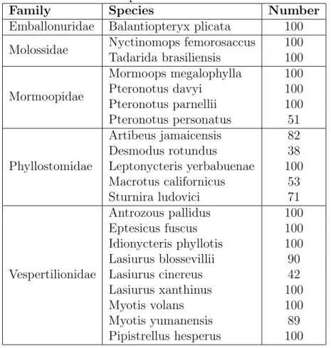
1.1 Description of the Selected Bat Data . . . 3

2.1 Results of the Shapiro-Wilk test with significance levelα= 0.05 for x . . . . 14

3.1 Prediction error (PE) . . . 26

3.2 Kernel naive Bayes . . . 28

3.3 SVM . . . 28

3.4 Multinomial probit model with Gaussian process prior . . . 29

List of Figures

1.1 Boxplot of the 20th-25th features after 0-1 normalization from species “Pterono-tus davyi” and “Pterono“Pterono-tus parnellii” . . . 4 2.1 Density estimation with Gaussian kernel for the (1,1)th vectorxi in Table 2.1 16

2.2 (a) Continuting splitting probability in a depth (b) Probability of different tree sizes . . . 19 3.1 Convergence diagnostics of GP over 5-Fold Cross Validation . . . 24 3.2 Convergence examinations of BART (for the 1st data in the test fold 1) . . 25

Acknowledgments

First and foremost, I would like to thank my thesis advisor Dr. Todd Kuffner. He encouraged and supported me in the searching of my thesis topic; invested his time and paid much attentions supervising me through weekly meeting and correspondences; and provided me valuable insights for my thesis. I would like to thank all the faculty members who have taught me. Thanks for your hard work and excellent lectures that introduce me to statistics. I would also like to thank the committee members, Dr. Kuffner and Dr. Lin for their time and guidance.

Last but not least, I would like to thank my family members and friends. I would not be able to overcome all the difficulties without your accompany. It is so great to have you in my life!

Zhongmao Liu

Washington University in Saint Louis May 2018

ABSTRACT OF THE THESIS

Bayesian Classification Methods for Bat Call Identification by

Zhongmao Liu Master of Art in Statistics

Washington University in St. Louis, May 2018 Research Advisor: Professor Todd Kuffner

Bat call classification is widely used in bat population monitoring in the field of ecology. Since bat populations are susceptible to changes in their surroundings, it is essential to monitor bat populations for purposes of bat protection and bio-environment protection. The purpose of this thesis is to compare the performance of several classification methods applied to a data set extracted from audio recordings for different species of bats in Mexico. The methods under comparison are (i) a nonparametric Bayesian approach using a multinomial probit model with Gaussian process prior; (ii) support vector machines (SVM); (iii) naive Bayes; and (iv) Bayesian additive regression trees (BART). We find that BART achieves the lowest classification error rate.

Chapter 1

Introduction

1.1

Introduction

Bats play an important role in the ecosystem. Some species of bat are productive polli-nators and seed dispersers (Hodgkison et al., 2003). Bats are beneficial to humans. Some species of bats are predators to many agricultural pests, such as tobacco budworm moths and cotton bollworm moths (Lee and McCracken, 2005). Furthermore, bats are useful in ecological research as their presence is an indicator of habitat quality (Kalcounis-Rueppell et al., 2007), including the human induced ecological change (Kunz et al., 2007), because bat populations are sensitive to global climate changes and human activities in their habitats such as urbanization, water quality and pesticide use (Jones et al., 2009).

Due to the vulnerability of bat populations to environmental changes, and their role as an ecological indicator, ecologists consider monitoring of bat populations to be an essential task. Among existing methods, acoustic monitoring is considered to be the most efficient. Acoustic monitoring involves making audio recordings of bat calls, and then developing a classifier based on data extracted from the audio recordings. An obstacle to acoustic monitoring is the lack of effective classification methods (Walters et al., 2013). In this thesis, we will compare

several classification methods to determine an effective procedure for classifying bat calls. The results of such an analysis would also have potential implications for classification of calls for other animals, such as birds..

Our data set consists of bat call data for 5 families and 21 species. The thesis is organized as follows. In Chapter 1, we introduce the bat call classification problem, then we provide a description of the data and discuss pre-processing. In Chapter 2, we illustrate four models for classification: multinomial probit model with Gaussian Process prior, support vector machines (SVM), naive Bayes and Bayesian sdditive regression trees. In Chapter 3, we implement the methods in R and present the results. In Chapter 4, we compared each methods and draw our conclusion.

1.2

Data Description and Pre-processing

The bat call data comes from Stathopoulos et al. (2014). The raw data are recordings of 8429 bat echolocation calls collected in Mexico. These bats are from 5 families, and each family contains one or more of the 21 different species. Each call is decomposed into a numeric vector containing 31 features using the software Sonobat 3.0.

Since the number of calls from some species are limited, we selected a maximum of 100 calls from each species and 1816 calls in total for modeling. The details of the selected data are shown in Table 1.1. Notice that when dividing the training and testing sets for 5-fold cross validation, we should do the random selection based on recordings rather than calls. The reason is that each recording may contain several calls from the same bat. It would be invalid to split the same bat’s calls into both the training and test sets (Stathopoulos et al.,

Table 1.1: Description of the Selected Bat Data

Family Species Number

Emballonuridae Balantiopteryx plicata 100

Molossidae Nyctinomops femorosaccus 100

Tadarida brasiliensis 100 Mormoopidae Mormoops megalophylla 100 Pteronotus davyi 100 Pteronotus parnellii 100 Pteronotus personatus 51 Phyllostomidae Artibeus jamaicensis 82 Desmodus rotundus 38 Leptonycteris yerbabuenae 100 Macrotus californicus 53 Sturnira ludovici 71 Vespertilionidae Antrozous pallidus 100 Eptesicus fuscus 100 Idionycteris phyllotis 100 Lasiurus blossevillii 90 Lasiurus cinereus 42 Lasiurus xanthinus 100 Myotis volans 100 Myotis yumanensis 89 Pipistrellus hesperus 100

2014). Under this restriction, the size of the 5 training sets are 1348, 1432, 1486, 1528, 1470, respectively; the size of 5 corresponding testing sets are 468, 384, 330, 288, 346, respectively.

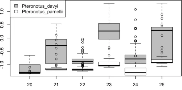
Before modeling, some pre-processing of the data is needed. First, since the range of each feature varies a lot, we use 0-1 normalization to adjust all the features to the same scale. Furthermore, the data set has missing values. There are a total of 21 missing values, which are coded as NA. These missing values are associated with 11 different calls, of which 2 are from “Pteronotus davyi” and 9 are from “Pteronotus parnellii”. All of the 21 NA values come from the 20th-25th feature. Considering that the maximum number of NAs from one

call is not larger than 2 (out of 31 total features), we have simply replaced the missing values with the corresponding species-level mean for that feature.

Figure 1.1 shows the boxplot of the 20th-25th feature’s data from species “Pteronotus davyi” and “Pteronotus parnellii” after 0-1 normalization. We can tell that the range of the two species varies considerably for each feature. Therefore for each missing value, we replace it with the mean for that feature and that species.

Figure 1.1: Boxplot of the 20th-25th features after 0-1 normalization from species “Pterono-tus davyi” and “Pterono“Pterono-tus parnellii”

Chapter 2

Statistical Models and Methods

This chapter introduces four classification methods. Details of model assumptions, defini-tions, inference procedures, and algorithms for implementation are included. The actual results are contained in Chapter 4.

2.1

Model Setup

Denote the observed data set as {(xi, yi)}, i = 1, . . . , N. The samples (xi, yi), for i =

1, . . . , N, are assumed to be independent of one another. Denote N×D numerical features’ matrix as X, where each observation xi ∈RD. Denote the N ×1 categorical vector of bat

2.2

Multinomial Probit Model with Gaussian Process

Priors

2.2.1

Likelihood Function

In addition to the observed data X and Y, we introduce an N ×K matrix M, which is composed of Gaussian Process random variablesmnk. Let mn denote thenth row of M and mk be thekth column of M. We also introduce anN ×K matrix Y∗, which is composed of

auxiliary variables y_nk∗ . Denote y_n∗ to be the nth row of Y∗ and y_k∗ to be the kth column of

Y∗. The multinomial probit model is as below :

y_nk∗ =mnk +, ∼N(0,1), yn=j if ynj∗ = max_0≤k≤K{y

∗

nk}.

(2.1)

Since the error is assumed to be standard normal, then this model implies that y_nk∗ |mnk ∼ N(mnk,1). From the second line in equation (2.1), we can deduce that P(yn = j|yn∗) = P(y_nj∗ >y∗_nk,∀k 6=j). Therefore, following (Girolami and Rogers, 2006), we have that

P(yn=j|mn) = Z P(yn =j|yn∗)P(y ∗ n|mn)dy∗n = Z P(y_nj∗ >y_nk∗ ,∀k 6=j) K Y k=1 P(y_nk∗ |mnk)dy∗n = Z +∞ −∞ P(y∗_nj|mnj)[ K Y k=1,k6=j Z y∗_nj −∞ P(y∗_nk|mnk)dynk∗ ]dy ∗ nj = Z +∞ −∞ P(y∗_nj|mnj) K Y k=1,k6=j Φ(y_nj∗ −mnk)dynj∗ . (2.2)

In equation (2.2), Φ(·) is the cumulative distribution function of the standard normal distri-bution. Let u=y_nj∗ −mnj, and hence u∼N(0,1). So equation (2.2) is equal to

P(yn =j|mn) = Z +∞ −∞ p(u) K Y k=1,k6=j Φ(u+mnj−mnk)du =_Eu[ K Y k=1,k6=j Φ(u+mnj −mnk)]. (2.3)

In a more concise form, we have

P(yn|mn) = Z K X j=1 P(y∗_nj>y_nk∗ ,∀k =6 j)I(yn =j)} K Y k=1 P(y∗_nk|mnk)dyn∗, and P(Y|M) = N Y n=1 P(yn|mn).

The likelihood function is given by

P(Y|M) = N Y n=1 nZ [ K X j=1 P(y_nj∗ >y_nk∗ ,∀k6=j)I(tn =j)] K Y k=1 P(y∗_nk|mnk)dyn∗ o . (2.4)

2.2.2

Gaussian Process Prior

Definition 1 A Gaussian process is a collection of random variables, any finite number of which have a joint Gaussian distribution (Rasmussen, 2004).

A Gaussian process can be defined by its mean functionm(x) and covariance functionk(x, x). The statement that f(x) follows a Gaussian process with specified mean and covariance is

expressed as

f(x)∼GP(m(x), k(x, x)).

Assume that for each column of M, mk is a Gaussian process composed of random variables m1k, ..., mN k. Assume that for each Gaussian Processmk, we havemk ∼GP(0,Σk), where0

is anN×1 zero vector and Σkis anN×N covariance matrix. The (i, j)th element in Σkis

de-fined asKk(xi, xj) = exp{− PD

d=1lkd(xid−xjd)2}. Writel= (l11, l12, . . . , l1D, . . . , lK1, lK2, . . . , lKD)T

to denote the parameters. When lkd →0, prior information extracted from x is small.

The prior distribution P(mk|X, l) is

P(mk|X, l)∼N(0,Σk),Σkij =Kk(xi, xj) = exp{− D X d=1 lkd(xid−xjd)2}. (2.5)

2.2.3

Inference

Let Θ = {Y∗_{, M}. Then the likelihood function is P(Y,Θ|X, l) =p(Y|M)p(M|X, l), where}

p(y|m) andp(m|X, l) are defined separately in equation (2.4) and equation (2.5), respectively. Note that the posterior is proportional to the likelihood, i.e. p(Θ|y, X, l)∝P(y,Θ|X, l). We can draw samples from the posterior via Gibbs Sampling (Girolami and Rogers, 2006).

Gibbs Sampling of Θ

Note that M and Y∗ are both N ×K matrices. Gibbs sampling for Θ(0),Θ(1), . . . ,Θ(s) proceeds as follows:

Algorithm 1Gibbs sampling for Θ

To initialize the algorithm,

(1) Generate M(0) _{according to m}(0) k ∼N(0,Σk) in equation (2.5). (2) Generate Y∗(0)|M(0) _{according to y}∗ n(0)|m (0) n ∼ Nyn(mn,1). Since yn∗(0)|mn follows a

truncated multivariate normal distribution, we should keep drawing new samples of the vector y_n∗(0) untily∗_nj > y_nk∗ , given yn=j.

For iterations 1,2, . . . ,s (1) Generate M(i+1)|Y∗(i) according tom(_ki+1)|y∗ k (i) _∼ N(Ckyk∗ (i) , Ck), Ck = Σk(I+ Σk)−1. (2) Generate Y∗(i+1)|M(i+1) _{according toy}∗ n (i+1)_|m(i+1) n ∼Nyn(m(ni+1),1). Prediction

Denote xnew as the new input. The prediction ofynew|xnew, X, y is

p(ynew=k|xnew, X, y) =

Z

p(ynew=k|mnew)p(mnew|xnew, X, y)dmnew. (2.6)

In equation (2.6), the first term can be derived from equation (2.2): P(ynew = j|mnew) = Eu[

QK

k=1,k6=jΦ(u+mnewj −mnewk )]. The second term,p(mnew|xnew, X, y) =N(mnew;µnew, σnew), will be presented later.

Although it is difficult to derive an analytic solution to the integral above, we can estimate the integral using Monte Carlo methods. This can be accomplished as follows:

Algorithm 2Prediction

(1) Draw Z samples of m from mk_new|y∗

k

(i)_{, X, y, x}

new ∼ N(µ, σ), where µ = (yk∗

(i)₎T_{(I +}

Σk)−1Σ12, σ = σnew − Σ21(I + Σk)−1Σ12, and where σnew, Σ12 and Σnew can be derived through the function Kk(·) because (m(_ki+1), mnew)T is Gaussian process.

(2) Estimate the function by ˆp(ynew = k|xnew, X, y) = _S1

PZ z=1Eu[ QK k=1,k6=jΦ(u+m new,z j − mnew,z_k )].

2.3

SVM

The support vector machine (SVM) was initially proposed as a binary classifier, but it also has applications in regression and ranking problems (Yu and Kim, 2012). The intuition for binary classification SVM is to divide the data into two different classes through a separating hyperplane, which has the largest margin between two classes. The margin (Yu and Kim, 2012) is the sum of the shortest distances from the hyperplane to the nearest points within each class.

2.3.1

Hard Margin SVM

Hard margin SVM correctly divides all data points when the classes are linearly separable. Consider a data set {(xi, yi)}, i = 1,2, ..., N with xi ∈ RD and yi ∈ {−1,1}. Define the

hyperplane classifier as f(x) = wT_{x+b, where w = (w}

1, . . . , wD) and b are parameters of

the hyperplane, such that

       f(xi)>0 if yi = 1 f(xi)<0 if yi =−1, (2.7) which is equivalent to yif(xi)>0.

Assume that yif(xi) =δ and δ>0. We can divide the inequality above by δ in both sides so

that yi(wTx+b)

δ =

δ

δ = 1. Thus the inequality can be rescaled to

Since the distance between a data point xi to the hyperplane is f(xi)/kwk (Yu and Kim,

2012), the margin is 1/kwk. Therefore, maximizing the margin is equivalent to minimizing

kwk. The hard margin SVM model is

min w,b 1 2w T_w s.t. yif(xi)>1, i= 1, . . . , n. (2.8)

The hard margin SVM is applicable only when the data is linearly separable. When the data is not linearly separable and such a hyperplane does not exist in the input space RD, there are 2 solutions: one is to use kernel methods to map the data from RD _{into higher}

dimension, in which linear separation is applicable; the other is to use soft margin SVM that allows mislabeled points.

2.3.2

Soft Margin SVM

Soft margin SVM solves an optimization problem with two goals: maximize the hyperplane’s margin and minimize the degree of misclassification. In our soft margin SVM model, we introduce the radial basis kernel functionφ(·) that mapsxi fromRDinto a higher-dimensional

space RN. The kernel function is defined as φ(xi, xj) = exp(−γkxi−xjk2), and we write φ(xi) = (φ(xi, x1), φ(xi, x2), . . . , φ(xi, xn)). Then we find a hyperplaneg(x) = wTφ(x)+b = 0

as in the hard margin SVM, however the hyperplane admits misclassified points. Further we introduce slack variables ξi with ξi > 0, and penalty parameter C (Yu and Kim, 2012).

When C is large, there will be a heavier penalty on misclassification and less importance placed on achieving a wide margin; whenC is small, there will be more misclassification and

a wider margin. The soft margin SVM model (Cortes and Vapnik, 1995) is min w,b,ξ 1 2w T_w+C n X i=1 ξi s.t. yig(xi)>1−ξi and ξi >0, i= 1, . . . , n. (2.9)

When solvingK-class classification problems, we can use the one versus all method (Nasrabadi, 2007). We trainK soft margin SVMs and obtain (w(1)_{, b}(1)_),(w(2)_{, b}(2)_{), ...,(w}(K)_{, b}(K)_{). Then} we assignynewto that classj having the largestg(j)(xnew) = (w(j))Tφ(xnew)+b(j), j = 1, ..., K.

2.4

Naive Bayes Classifier

Naive Bayes is a simple classifier. It is based on an assumption: all the features are mutually independent given the lable. Although this assumption is not usually satisfied, naive Bayes still performs well in many problems. There are at least three naive Bayes methods for continuous data (Bouckaert, 2004). To approximate feature variables’ distribution, the classic Naive Bayes assume that the data follows certain distributions, such as Gaussian or gamma. Kernel Naive Bayes uses nonparametric estimation of the feature distributions (John and Langley, 1995). Discretization Naive Bayes discretizes the continuous data (Dougherty et al., 1995).

2.4.1

Model Notations and Definitions

Define the data set as {(xi, yi)}, i = 1, ..., N, as in section 2.1. Based on the assumption

that each feature is independent, we have

p(xi|yi =k) =p(xi1|xi2, ..., xiD, yi =k)p(xi2|xi3, ..., xiD, yi =k)...(xiD|yi =k) = D Y j=1 p(xij|yi =k).

We can deduce the posterior of yi as

p(yi =k|xi) = p(yi =k)p(xi|yi =k) p(xi) ∝p(yi =k)p(xi|yi =k) =p(yi =k) D Y j=1 p(xij|yi =k), (2.10) and ˆyi =j if p(yi =j|xi) = maxk∈Kp(yi =k|xi).

To approximate p(yi = k), we can use ˆp(yi = k) = n_Nk, where nk is the number of data

points withy=k. Then we need to approximate the distribution of the continuous random variable x|y.

2.4.2

Classic Naive Bayes

For notational simplicity, we denote the D× K vectors of x[,j]|y = k, j = 1, . . . , D, k = 1, ..., K’s as x1, x2, . . . , xDK. Denote Si as the length of the each vector xi, i = 1, . . . , DK.

usually a normal distribution p(xi) = N(xi;µi, σi). In the following, we conduct normality

tests for each of the D×K vectors ofxi.

We choose the Shapiro-Wilk test to examine if the normality assumption stands, because it is a more powerful method compared to many other widely-used normality tests, such as the Kolmogorov Smirnov test, the Lilliefors test and the Anderson Darling test (Mohd Razali and Yap, 2011). The null hypothesis of the Shapiro-Wilk normality test (Shapiro and Wilk, 1965) is: all the samples xi1, xi2, . . . , xiSi within a vectorxicome from a normally distributed

population. The test statistic isWi =

(PSi j=1aijx(ij))2 PSi j=1(xij−¯xi)2 , with (ai1, . . . , aiSi) = mT_V−1 (mT_V−1_V−1_m)12 ,x(ij) being the jth smallest observation in xi, m = (m1, . . . , mSi)

T _{being the expected values of}

ordered variables sampled from the standard normal distribution, andV being the covariance matrix of m. The results of the Shapiro-Wilk tests are presented in Table 2.1.

Table 2.1: Results of the Shapiro-Wilk test with significance level α= 0.05 for x

1 1 2 3 4 5 6 7 8 9 10 11 12 13 14 15 16 17 18 19 20 21 22 23 24 25 26 27 28 29 30 31 1 1 1 1 1 1 1 1 1 1 1 1 1 2 1 1 1 1 1 1 1 1 1 3 1 1 1 1 1 1 1 1 1 1 1 1 1 1 1 4 1 1 1 1 1 1 1 1 1 5 1 1 1 1 1 1 1 1 1 1 1 6 1 1 1 1 7 1 1 1 1 1 8 1 1 1 1 1 1 1 9 1 1 1 1 1 1 1 1 1 1 1 1 1 1 1 1 1 1 1 10 1 1 1 1 1 1 11 1 1 1 1 1 1 12 1 1 1 1 1 1 1 1 1 1 13 1 1 1 1 1 1 1 1 1 1 1 1 14 1 1 1 1 1 1 1 15 1 1 1 1 1 1 1 1 16 1 1 1 1 1 1 1 1 1 17 1 1 1 1 1 18 1 1 1 19 1 1 1 1 1 1 1 20 1 1 1 1 1 1 1 1 1 21 1 1 1 1 1 1 1 1 1 1 1 1 1 1 1 1 1 1 1 1

This is the results of the Shapiro-Wilk normality test for 21×31 vectors of x. When the

p value<0.05, H0 is rejected and 0 is returned; when pvalue>0.05, H0 is not rejected, and 1 is returned.

Table 2.1 shows the results of the Shapiro-Wilk tests. Note that at significance levelα= 0.05, the null hypothesis of normality is rejected for more than half of the vectors xi. Thus, we

have found evidence against the assumption of normality employed in the classical naive Bayes classification model.

2.4.3

Kernel Naive Bayes

Next, we apply the kernel naive Bayes model to our data. In the kernel naive Bayes model, we use nonparametric kernel density estimates of the distributions of the predictor variables (John and Langley, 1995). These nonparametric estimators have the advantage that they can accurately estimate any unknown density or distribution function within a broad class of candidate functions. However in the classical naive Bayes approach above, a parametric assumption of normality is assumed for these distributions. The distribution of each vector

xi is approximated as P(xi) = 1 Si Si X j=1 N(xij;µij, σ).

We approximate each mean value µij with ˆµij = xij. The kernel bandwidth determines

the relevant neighborhood, and hence the relevant data points, for estimating the density function at a given input value. To specify the bandwidth parameter, we follow Silverman’s rule of thumb (Silverman, 1986): ˆσ = 0.9S−

1 5

i ×min{sd(xi),Q0.75(xi

)−Q0.25(xi)

1.34 }, whereQ0.25(xi) and Q0.75(xi) are, respectively, the 0.25 and 0.75 quantiles of xi.

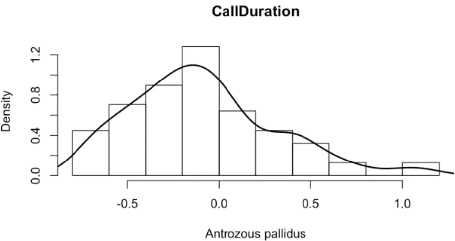
The density estimate shown in Figure 2.1 suggests that the distribution of the call duration, i.e. the first feature, of Antrozous pallidus is far from the normal distribution. Therefore, compared to the assumed normal distribution for this feature, the kernel density estimate (with Gaussian kernel) seems to be a better approximation to the true feature distribution.

Figure 2.1: Density estimation with Gaussian kernel for the (1,1)th vector xi in Table 2.1

2.5

Bayesian Additive Regression Tree (BART)

Another popular classification method is referred to as classification and regression trees (CART); the name appears to have originated with Breiman (2017). CART works through recursively dividing the data based on the input values ofx. Each input goes through the tree from the root node to a leaf node, and finally a value related to each leaf node is returned.

Chipman et al. (1998) applied Bayesian ideas to CART, by assigning a prior distribution to the trees and model parameters. They further proposed Bayesian additive regression trees (BART), which utilize sums of trees rather than a single tree. BART defines the continuous response variabley∗ to be the sum of regression trees and a normal random error (Chipman et al., 2010). Zhang and H¨ardle (2010) adapted BART to classification problems.

2.5.1

Model Notations and Definitions

We begin with the binary classification case. As before, the data set is {(xi, yi)}, i =

1,2, . . . , N with xi ∈ RD and yi ∈ {0,1}. We introduce a latent (unobserved)

continu-ous variable Y∗ and construct the latent probit model as

       Y = 1, if Y∗ _>0, Y = 0, if Y∗<0. (2.11)

The number of trees to be built is denoted bym. Write Ti to denote a binary regression tree

with a number Bi of terminal nodes. Further, Mi ={µi1, . . . , µiBi} denotes the predictions

to be returned from each terminal node, respectively. Suppose ∼N(0,1). The parameter to be estimated is Θ = (T1, . . . , Tm, M1, . . . , Mm), i = 1, . . . , m. The function g(x;Ti, Mi)

returns the predicted valueµij when data x goes through the treeTi. Following Zhang and

H¨ardle (2010), construct the additive regression tree as

y∗ =

m X

i=1

g(x:Ti, Mi) +, ∼N(0,1).

We can deduce that P(y= 1|x, T, M) = P(y∗>0|x, T, M) = Φ[Pm

2.5.2

Prior Specification

Assume that each tree is independent. The joint prior density for the additive tree model is

P((T1, M1),(T2, M2), ...,(TM, Mm)) = m Y i=1 p(Ti, Mi) = m Y i=1 p(Mi|Ti)p(Ti) = m Y i=1 p(Ti) Bi Y j=1 p(µij|Ti). (2.12) 2.5.2.1 The Ti Prior

A regression tree is built through two functions Psplit(·) and Prule(·) (Chipman et al., 1998). While building a tree Ti, Psplit(η, Ti) defines the probability that the node η will further

split into two new nodes rather than end as a leaf node; Prule(ρ|η, Ti) is the probability of

assigning splitting rule ρ to node η.

In a single regression tree, we need the tree to be large enough (have enough leaf nodes) to capture the complex structure of the data. By contrast, in an additive tree model, we want to keep each tree small, especially when m is large. We may control the size of a tree using a splitting rule (Chipman et al., 1998):

Psplit(d) =α(1 +d)−β, α∈(0,1), β ∈[0,+∞),

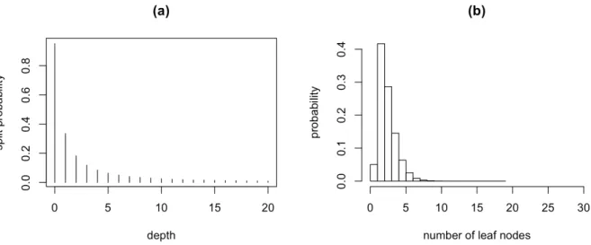
where d is the depth of the node. The splitting probability Psplit(d) decreases as d grows. According to Chipman et al. (1998), we set α = 0.95, β = 2. Panel (a) in Figure 2.2 shows the density function of P (d) with α= 0.95, β= 2. Observe that the splitting probability

decreases as the depth increases. Then we run 1000 simulations to build a tree based on

Psplit(·), and present the result in Panel (b). The figure shows that the tree is most likely to end in 2, 3 or 4 lead nodes.

Figure 2.2: (a) Continuting splitting probability in a depth (b) Probability of different tree sizes

In a regression tree, the splitting rulePrule(·) includes 2 components: choosing featurexi and

choosing split value s. We set the splitting rule as choosing feature iaccording to a uniform distribution on the set of all features, and choosings according to a uniform distribution on the set of observed values of xi (Chipman et al., 1998).

2.5.2.2 The µij|Ti Prior

Assume that µij|Tj follows a conjugate normal distribution µij|Ti ∼ N(0, σµ2), such that E(Y∗)∼N(0, mσ2

µ) (Chipman et al., 1998). We may specify the interval [E[y

∗_]

min, E[y∗]max]=[−3,3], and the range of observed E[y∗] to span k standard deviations. We can deduce k√mσµ =

ymax= 3. Thus the hyperparameter σµ is set to the value 3/k √

towards 0 as m grows. Moreover, when shrinkingµij to 0, P(x) is also shrunk towards 0.5.

Settingk = 2, the prior µij|Tj is

µij|Ti ∼N(0, σµ2), σµ = 3/2 √

m.

2.5.3

Posterior Simulation and Inference

The posterior is P((T1, M1),(T2, M2), . . . ,(Tm, Mm)|x, y). We use backfitting MCMC

al-gorithm (Albert and Chib, 1993) to draw samples from the posterior density of Θ(s) ₌ (T₁(s), ..., Tm(s), M₁(s), . . . , Mm(s)), s = 1,2, . . . , S. Take Y∗ as a missing value and generate the N ×1 vector y∗ from observed data:

       y∗(s)|y= 1 ∼max{N(Pm i=1g(x:Ti, Mi)(s),1),0} y∗(s)|y= 0 ∼min{N(Pm i=1g(x:Ti, Mi)(s),1),0}. (2.13)

Write Ti to denote the ith tree and Mi to denote the ith tree’s returned values. Further,

write T(i) to denote the set of all trees with the ith tree deleted, and similarly write M(i) to denote the set of all returned values with the ith tree’s returned values deleted. Draw a posterior sample (Ti, Mi)(s+1) by sampling successively from the conditional distributions

(Ti, Mi)(s+1)|T (s) (i), M (s) (i), y ∗(s) .

The posterior samples (T1, M1)(s),(T2, M2)(s), . . . ,(Tm, Mm)(s)represent samples from a Markov

chain that is converging to a stationary distribution that is the same as the distribution cor-responding to the true additive trees, i.e. the true posterior distribution. Based on each draw

of additive trees, the prediction for new inputxnewcan be made by the following probability: ˆ p(s)(xnew) = Φ( m X i=1 ˆ g(xnew, T (s) i , M (s) i )).

After a burn-in period, we compute the average of S probability values to obtain the final prediction given by ˆ P(xnew) = S X s=1 ˆ p(s)(xnew).

For theK-class classification problem, we can build K BART classifiers, and then attribute

Chapter 3

Numerical Results

We use the R package “vbmp” to implement the multinomial probit model with Gaussian process prior (GP); package “e1070” to implement the soft margin SVM, package “naive-bayes” to implement the kernel naive Bayes; package “BayesTree” to implement the binary BART and then one versus all method for theK-class classification (BART). As presented in section 1.2, the data set is divided into 5 training and testing sets for 5-fold cross validation.

3.1

Running Time

The Running time for the soft margin SVM and the kernel naive Bayes are short. It takes either of the two models less than 3 seconds to go through the 5-fold cross validation. The Running time for GP is moderate, which is around 9 minutes. The running time for BART is long, which is about 3 hours. Since we use the one versus all method while conducting BART model, 21 binary classification model will be trained in BART rather than just 1 model in GP in each cross validation fold. However, the exact running time for BART still depends on the iterations of MCMC.

3.2

Convergence Examination

Convergence examination is essential while conducting GP and BART. When conducting GP, we set l1 = . . . = lKD = 1. Figure 3.1 shows the convergence diagnostics of GP over

5-fold cross validation separately. There is no reason to reject convergence after 14 iterations for all of the 5-fold cross validation.

Implementing the binary BART involves calculating a single probability ˆp(s)_(x

new) with MCMC. In our multi-class classification case with number of specie K = 21, the BART requires calculating K probabilities, one for each specie. We set S = 3000 with burn-in 0. Figure 3.2 shows the MCMC trace plots of these probabilities for each of the 21 specie, where

xnew is the 1st data in test fold 1. After checking the trace plots, we finally set S = 1100 with burn-in 100.

3.3

Prediction error

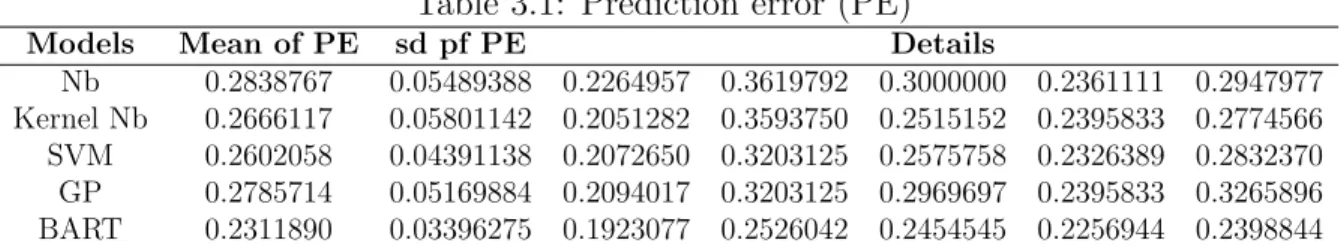
Table 3.1 shows the prediction errors of our models on the bat call data. We find that after applying kernels, the prediction performance of naive Bayes are improved a lot. The prediction accuracy is even higher than GP. In all, the performance of kernel naive Bayes, SVM and GP are close to each other, while the BART model performs much better than the former three.

Table 3.1: Prediction error (PE)

Models Mean of PE sd pf PE Details

Nb 0.2838767 0.05489388 0.2264957 0.3619792 0.3000000 0.2361111 0.2947977

Kernel Nb 0.2666117 0.05801142 0.2051282 0.3593750 0.2515152 0.2395833 0.2774566

SVM 0.2602058 0.04391138 0.2072650 0.3203125 0.2575758 0.2326389 0.2832370

GP 0.2785714 0.05169884 0.2094017 0.3203125 0.2969697 0.2395833 0.3265896

BART 0.2311890 0.03396275 0.1923077 0.2526042 0.2454545 0.2256944 0.2398844

The columns are the mean of prediction errors, standard deviations of the prediction errors, and the prediction errors of the 5-fold cross validation, separately.

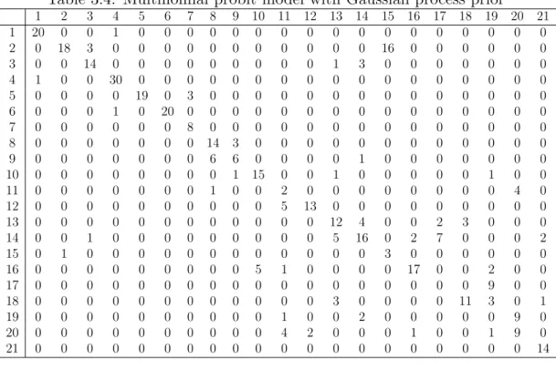
3.4

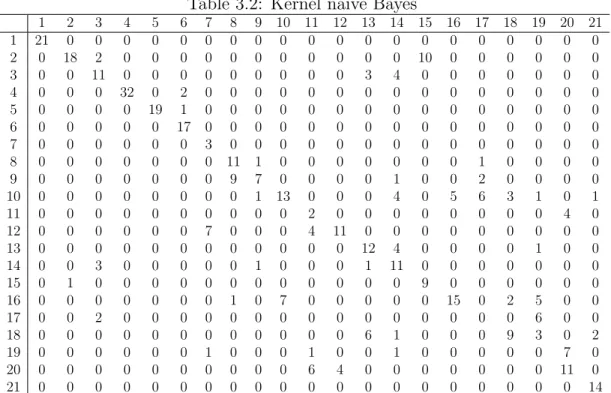
Crossing Table

By drawing crossing tables, we look into the prediction performance of the four models on the seconed test data, on which all of the four models perform the worst. Table 3.2 - 3.5 are the crossing tables of kernel Naive Bayes, SVM, GP model and BART, separately. The columns of each crossing table are true specie name and rows are predicted specie name. From the four crossing tables we can find that:

•The prediction accuracy of the families 1, 2 and 3 are high for all of the four models, which means that the bats from families 1, 2 and 3 can be easily distinguished by any of the four models.

• Most misclassification cases are from families 4 and 5. The misclassification rates within family 5 and between families 4 and 5 are high.

•The misclassification rate of the 11th, 15th (except from BART), 17th and 19th specie are higher than 50%, which is because for these specie, some of their features’ range in the test set differ from that in the training set, or even highly overlap with that of other specie.

• BART seems to be the best model for bat call classification among the four models, because it has the smallest prediction error. More importantly, BART is less likely to divide the data from familiy 4 and familiy 5 out of the two classes, which is helpful for conducting reclassification of the data that are classified into the two families.

Table 3.2: Kernel naive Bayes 1 2 3 4 5 6 7 8 9 10 11 12 13 14 15 16 17 18 19 20 21 1 21 0 0 0 0 0 0 0 0 0 0 0 0 0 0 0 0 0 0 0 0 2 0 18 2 0 0 0 0 0 0 0 0 0 0 0 10 0 0 0 0 0 0 3 0 0 11 0 0 0 0 0 0 0 0 0 3 4 0 0 0 0 0 0 0 4 0 0 0 32 0 2 0 0 0 0 0 0 0 0 0 0 0 0 0 0 0 5 0 0 0 0 19 1 0 0 0 0 0 0 0 0 0 0 0 0 0 0 0 6 0 0 0 0 0 17 0 0 0 0 0 0 0 0 0 0 0 0 0 0 0 7 0 0 0 0 0 0 3 0 0 0 0 0 0 0 0 0 0 0 0 0 0 8 0 0 0 0 0 0 0 11 1 0 0 0 0 0 0 0 1 0 0 0 0 9 0 0 0 0 0 0 0 9 7 0 0 0 0 1 0 0 2 0 0 0 0 10 0 0 0 0 0 0 0 0 1 13 0 0 0 4 0 5 6 3 1 0 1 11 0 0 0 0 0 0 0 0 0 0 2 0 0 0 0 0 0 0 0 4 0 12 0 0 0 0 0 0 7 0 0 0 4 11 0 0 0 0 0 0 0 0 0 13 0 0 0 0 0 0 0 0 0 0 0 0 12 4 0 0 0 0 1 0 0 14 0 0 3 0 0 0 0 0 1 0 0 0 1 11 0 0 0 0 0 0 0 15 0 1 0 0 0 0 0 0 0 0 0 0 0 0 9 0 0 0 0 0 0 16 0 0 0 0 0 0 0 1 0 7 0 0 0 0 0 15 0 2 5 0 0 17 0 0 2 0 0 0 0 0 0 0 0 0 0 0 0 0 0 0 6 0 0 18 0 0 0 0 0 0 0 0 0 0 0 0 6 1 0 0 0 9 3 0 2 19 0 0 0 0 0 0 1 0 0 0 1 0 0 1 0 0 0 0 0 7 0 20 0 0 0 0 0 0 0 0 0 0 6 4 0 0 0 0 0 0 0 11 0 21 0 0 0 0 0 0 0 0 0 0 0 0 0 0 0 0 0 0 0 0 14 Table 3.3: SVM 1 2 3 4 5 6 7 8 9 10 11 12 13 14 15 16 17 18 19 20 21 1 21 0 0 0 0 0 0 0 0 0 0 0 0 0 0 0 0 0 0 0 0 2 0 17 3 0 0 0 0 0 0 0 0 0 0 0 14 0 0 0 0 0 0 3 0 0 12 0 0 0 0 0 0 0 0 0 2 2 0 0 0 0 0 0 0 4 0 0 0 30 0 0 0 0 0 0 0 0 0 0 0 0 0 0 0 0 0 5 0 0 0 0 19 0 0 0 0 0 0 0 0 0 0 0 0 0 0 0 0 6 0 0 0 2 0 20 0 0 0 0 0 0 0 0 0 0 0 0 0 0 0 7 0 0 0 0 0 0 11 0 0 0 0 0 0 0 0 0 0 0 0 0 0 8 0 0 0 0 0 0 0 17 7 0 0 0 0 0 0 0 0 0 0 1 0 9 0 0 0 0 0 0 0 3 2 0 0 0 0 0 0 0 0 0 0 0 0 10 0 0 0 0 0 0 0 0 1 15 0 0 0 2 0 4 1 0 2 0 1 11 0 0 0 0 0 0 0 1 0 0 2 0 0 0 0 0 0 0 0 3 0 12 0 0 0 0 0 0 0 0 0 0 4 13 0 0 0 0 0 0 0 0 0 13 0 0 0 0 0 0 0 0 0 0 0 0 12 4 0 0 3 4 1 0 0 14 0 0 0 0 0 0 0 0 0 0 0 0 1 17 0 0 4 0 0 0 0 15 0 2 0 0 0 0 0 0 0 0 0 0 0 0 5 0 0 0 0 0 0 16 0 0 0 0 0 0 0 0 0 5 0 0 0 0 0 16 1 0 2 0 0 17 0 0 1 0 0 0 0 0 0 0 0 0 0 0 0 0 0 0 9 0 0 18 0 0 2 0 0 0 0 0 0 0 0 0 7 0 0 0 0 10 2 0 2 19 0 0 0 0 0 0 0 0 0 0 1 0 0 1 0 0 0 0 0 10 0 20 0 0 0 0 0 0 0 0 0 0 6 2 0 0 0 0 0 0 0 8 0 21 0 0 0 0 0 0 0 0 0 0 0 0 0 0 0 0 0 0 0 0 14

Table 3.4: Multinomial probit model with Gaussian process prior 1 2 3 4 5 6 7 8 9 10 11 12 13 14 15 16 17 18 19 20 21 1 20 0 0 1 0 0 0 0 0 0 0 0 0 0 0 0 0 0 0 0 0 2 0 18 3 0 0 0 0 0 0 0 0 0 0 0 16 0 0 0 0 0 0 3 0 0 14 0 0 0 0 0 0 0 0 0 1 3 0 0 0 0 0 0 0 4 1 0 0 30 0 0 0 0 0 0 0 0 0 0 0 0 0 0 0 0 0 5 0 0 0 0 19 0 3 0 0 0 0 0 0 0 0 0 0 0 0 0 0 6 0 0 0 1 0 20 0 0 0 0 0 0 0 0 0 0 0 0 0 0 0 7 0 0 0 0 0 0 8 0 0 0 0 0 0 0 0 0 0 0 0 0 0 8 0 0 0 0 0 0 0 14 3 0 0 0 0 0 0 0 0 0 0 0 0 9 0 0 0 0 0 0 0 6 6 0 0 0 0 1 0 0 0 0 0 0 0 10 0 0 0 0 0 0 0 0 1 15 0 0 1 0 0 0 0 0 1 0 0 11 0 0 0 0 0 0 0 1 0 0 2 0 0 0 0 0 0 0 0 4 0 12 0 0 0 0 0 0 0 0 0 0 5 13 0 0 0 0 0 0 0 0 0 13 0 0 0 0 0 0 0 0 0 0 0 0 12 4 0 0 2 3 0 0 0 14 0 0 1 0 0 0 0 0 0 0 0 0 5 16 0 2 7 0 0 0 2 15 0 1 0 0 0 0 0 0 0 0 0 0 0 0 3 0 0 0 0 0 0 16 0 0 0 0 0 0 0 0 0 5 1 0 0 0 0 17 0 0 2 0 0 17 0 0 0 0 0 0 0 0 0 0 0 0 0 0 0 0 0 0 9 0 0 18 0 0 0 0 0 0 0 0 0 0 0 0 3 0 0 0 0 11 3 0 1 19 0 0 0 0 0 0 0 0 0 0 1 0 0 2 0 0 0 0 0 9 0 20 0 0 0 0 0 0 0 0 0 0 4 2 0 0 0 1 0 0 1 9 0 21 0 0 0 0 0 0 0 0 0 0 0 0 0 0 0 0 0 0 0 0 14 Table 3.5: BART 1 2 3 4 5 6 7 8 9 10 11 12 13 14 15 16 17 18 19 20 21 1 21 0 0 0 0 0 0 0 0 0 0 0 0 0 0 0 0 0 0 0 0 2 0 19 3 0 0 0 0 0 0 0 0 0 0 0 0 0 0 0 0 0 0 3 0 0 14 0 0 0 0 0 0 0 0 0 1 2 0 0 0 0 0 0 0 4 0 0 0 32 0 1 0 0 0 0 0 0 0 0 0 0 0 0 0 0 0 5 0 0 0 0 19 0 0 0 0 0 0 0 0 0 0 0 0 0 0 0 0 6 0 0 0 0 0 19 0 0 0 0 0 0 0 0 0 0 0 0 0 0 0 7 0 0 0 0 0 0 10 0 0 0 0 0 0 0 0 0 0 0 0 0 0 8 0 0 0 0 0 0 0 21 4 0 0 0 0 1 0 0 0 0 0 0 0 9 0 0 0 0 0 0 0 0 1 0 0 0 0 0 0 0 0 0 0 0 0 10 0 0 0 0 0 0 0 0 4 15 0 0 0 1 0 3 2 0 2 0 0 11 0 0 0 0 0 0 0 0 0 0 2 0 0 0 0 0 0 0 0 4 0 12 0 0 0 0 0 0 1 0 0 0 5 11 0 0 0 0 0 0 0 0 0 13 0 0 0 0 0 0 0 0 0 0 0 0 13 2 0 0 3 0 3 0 0 14 0 0 0 0 0 0 0 0 1 0 0 0 1 17 0 0 3 0 0 0 0 15 0 0 0 0 0 0 0 0 0 0 0 0 0 0 19 0 0 0 0 0 0 16 0 0 0 0 0 0 0 0 0 4 0 0 0 0 0 17 1 0 3 0 0 17 0 0 1 0 0 0 0 0 0 0 0 0 0 0 0 0 0 0 4 0 0 18 0 0 0 0 0 0 0 0 0 0 0 0 7 1 0 0 0 14 4 0 2 19 0 0 0 0 0 0 0 0 0 1 1 0 0 2 0 0 0 0 0 10 0 20 0 0 0 0 0 0 0 0 0 0 5 4 0 0 0 0 0 0 0 8 0 21 0 0 0 0 0 0 0 0 0 0 0 0 0 0 0 0 0 0 0 0 15

Chapter 4

Conclusion

All of the classification models we applied in this thesis are useful in bat call identification. They have classification accuracies from 71% to 77% in our bat call data .

Among the four models, kernel naive Bayes and SVM have the advantage of short running time. BART has superior classification accuracy than the other three models. However, it takes significantly more time to train the data. After comparing all the aspects of the models’ performances, we consider BART to be the best one among the four models to conduct bat call identification. Since it has the highest classification accuracy and performs the best in dividing the first three families from the last two, which should be helpful if we were to conduct reclassification in the last two families.

There are several ways to improve the classification accuracy. One is to increase the size of training data, so we can have more knowledge on the properties of different bat specie. The second is to add more acoustic features to our data. Since the misclassifications come par-tially from the overlapping in features’ range among different specie, adding in new features and screening the old features should be useful in further identification of bats from family 4 and family 5.

References

James H Albert and Siddhartha Chib. Bayesian analysis of binary and polychotomous response data.Journal of the American statistical Association, 88(422):669–679, 1993.

Remco R Bouckaert. Naive bayes classifiers that perform well with continuous variables. In Australasian Joint Conference on Artificial Intelligence, pages 1089–1094. Springer, 2004.

Leo Breiman. Classification and regression trees. Routledge, 2017.

Hugh A Chipman, Edward I George, and Robert E McCulloch. Bayesian cart model search. Journal of the American Statistical Association, 93(443):935–948, 1998.

Hugh A Chipman, Edward I George, Robert E McCulloch, et al. Bart: Bayesian additive regression trees.

The Annals of Applied Statistics, 4(1):266–298, 2010.

Corinna Cortes and Vladimir Vapnik. Support-vector networks. Machine learning, 20(3):273–297, 1995. James Dougherty, Ron Kohavi, and Mehran Sahami. Supervised and unsupervised discretization of

contin-uous features. InMachine Learning Proceedings 1995, pages 194–202. Elsevier, 1995.

Mark Girolami and Simon Rogers. Variational bayesian multinomial probit regression with gaussian process priors. Neural Computation, 18(8):1790–1817, 2006.

Robert Hodgkison, Sharon T Balding, Akbar Zubaid, and Thomas H Kunz. Fruit bats (chiroptera: Pteropo-didae) as seed dispersers and pollinators in a lowland malaysian rain forest. Biotropica, 35(4):491–502, 2003.

George H John and Pat Langley. Estimating continuous distributions in bayesian classifiers. InProceedings of the Eleventh conference on Uncertainty in artificial intelligence, pages 338–345. Morgan Kaufmann Publishers Inc., 1995.

Gareth Jones, David S Jacobs, Thomas H Kunz, Michael R Willig, and Paul A Racey. Carpe noctem: the importance of bats as bioindicators. Endangered species research, 8(1-2):93–115, 2009.

MC Kalcounis-Rueppell, VH Payne, SR Huff, and AL Boyko. Effects of wastewater treatment plant effluent on bat foraging ecology in an urban stream system. Biological Conservation, 138(1-2):120–130, 2007. Thomas H Kunz, Edward B Arnett, Wallace P Erickson, Alexander R Hoar, Gregory D Johnson, Ronald P

Larkin, M Dale Strickland, Robert W Thresher, and Merlin D Tuttle. Ecological impacts of wind energy development on bats: questions, research needs, and hypotheses. Frontiers in Ecology and the Environ-ment, 5(6):315–324, 2007.

Ya-Fu Lee and Gary F McCracken. Dietary variation of brazilian free-tailed bats links to migratory popu-lations of pest insects. Journal of Mammalogy, 86(1):67–76, 2005.

Nornadiah Mohd Razali and Bee Yap. Power comparisons of shapiro-wilk, kolmogorov-smirnov, lilliefors and anderson-darling tests. 2, 01 2011.

Carl Edward Rasmussen. Gaussian processes in machine learning. InAdvanced lectures on machine learning, pages 63–71. Springer, 2004.

S. S. Shapiro and M. B. Wilk. An analysis of variance test for normality (complete samples). Biometrika, 52(3/4):591–611, 1965. ISSN 00063444. URLhttp://www.jstor.org/stable/2333709.

Bernard W Silverman. Density estimation for statistics and data analysis, volume 26. CRC press, 1986. Vassilios Stathopoulos, Veronica Zamora-Gutierrez, Kate Jones, and Mark Girolami. Bat call identification

with gaussian process multinomial probit regression and a dynamic time warping kernel. In Artificial Intelligence and Statistics, pages 913–921, 2014.

Charlotte L Walters, Alanna Collen, Tim Lucas, Kim Mroz, Catherine A Sayer, and Kate E Jones. Challenges of using bioacoustics to globally monitor bats. InBat evolution, ecology, and conservation, pages 479–499. Springer, 2013.

Hwanjo Yu and Sungchul Kim. Svm tutorialclassification, regression and ranking. InHandbook of Natural computing, pages 479–506. Springer, 2012.

Junni L Zhang and Wolfgang K H¨ardle. The bayesian additive classification tree applied to credit risk modelling. Computational Statistics & Data Analysis, 54(5):1197–1205, 2010.