Training Data Generation Framework For Machine-Learning Based Classifiers

(1)

Digital WPI

Masters Theses (All Theses, All Years)

Electronic Theses and Dissertations

2018-12-14

Training Data Generation Framework For

Machine-Learning Based Classifiers

Kyle W. McClintick

Worcester Polytechnic Institute, [email protected]

Follow this and additional works at:

https://digitalcommons.wpi.edu/etd-theses

This thesis is brought to you for free and open access byDigital WPI. It has been accepted for inclusion in Masters Theses (All Theses, All Years) by an authorized administrator of Digital WPI. For more information, please [email protected].

Repository Citation

McClintick, Kyle W., "Training Data Generation Framework For Machine-Learning Based Classifiers" (2018).Masters Theses (All Theses, All Years). 1276.

(2)

by

Kyle W. McClintick

A Thesis

Submitted to the Faculty of the

WORCESTER POLYTECHNIC INSTITUTE in partial fulfillment of the requirements for the

Degree of Master of Science in

Electrical and Computer Engineering by

December 2018

APPROVED:

Professor Alexander Wyglinski, Major Advisor

Professor Wickramarathne Thanuka

(3)

In this thesis, we propose a new framework for the generation of training data for machine learning techniques used for classification in communications applications.

Machine learning-based signal classifiers do not generalize well when training data does not describe the underlying probability distribution of real signals. The simplest way to accomplish statistical simi-larity between training and testing data is to synthesize training data passed through a permutation of plausible forms of noise. To accomplish this, a framework is proposed that implements arbitrary channel conditions and baseband signals. A dataset generated using the framework is considered, and is shown to be appropriately sized by having 11% lower entropy than state-of-the-art datasets.

Furthermore, unsupervised domain adaptation can allow for powerful generalized training via deep fea-ture transforms on unlabeled evaluation-time signals. A novel Deep Reconstruction-Classification Network (DRCN) application is introduced, which attempts to maintain near-peak signal classification accuracy despite dataset bias, or perturbations on testing data unforeseen in training.

Together, feature transforms and diverse training data generated from the proposed framework, teaching a range of plausible noise, can train a deep neural net to classify signals well in many real-world scenarios despite unforeseen perturbations.

(4)

Acknowledgements

I would like to express my deepest gratitude to my advisor Professor Alexander Wyglinski for his continuous guidance and support towards my degree. I am very thankful for the opportunity to work

with him in the Wireless Innovation Laboratory at Worcester Polytechnic Institute.

I want to thank Professor Wickramarathne Thanuka and Professor Donald Brown for serving on my committee and providing valuable suggestions and comments with regards to my thesis. I would like to thank James Kingsley, scientific computing system specialist, and Spencer Pruitt,

computational scientist from the WPI Academic and Research Computing group at Worcester Polytechnic Institute. Consulting and GPU cluster computing support from the WPI Academic and

Research Computing Group contributed to results reported within this thesis.

I would also like to thank my Wilab team members Dr. Srikanth Pagadarai, Kuldeep, Renato, and Nivetha for their immense support during my graduate studies. I would like to thank my friends abroad and in the states who have stayed in contact and given me the support I need, including my room-mates

from Terre Haute. I would like to thank good beer, catchy music, and sunny weekends. Finally, I’m thankful for my lovely girlfriend Zhijie, and my warm family: Colin, Dawn, and George.

(5)

List of Figures

2.1 A flow chart of a transmit and receive chain of communications tasks. Arrows indicate movement of information from one block to another. The form that information takes at each step is communicated through annotations. Antennas are pictured as upside-down triangles. . . 8 2.2 The discrete delay channel model, adapted from [1]. Inputs each have isolated time delays

τi, ray powers |βi|2 =A0ai/di, and ray phasesejφi. . . 11

2.3 Bluetooth Pr (2.11) observed by a receiver (See Appendix A.1) from a single car over a

50 m stretch of road, whose reflections correspond to the scenario described in Figure 2.4. Significant fluctuations occur frequently due to phase interference. . . 12 2.4 Physical Characteristics of the 5-reflection 3D Doppler channel. The paths are attenuated

assuming the ground path is dry asphalt[ref] (a5 = 0.34), the roadsides are concrete (a3 = 0.38), and the cars are metallic (a2,4 = 0.8). The direct path is not attenuated by reflection (a1 = 1). Blue-tooth sources are placed at a height of 1.5 m and the receiver at a height of 5m.. . . 13 2.5 Blue-toothPr (2.11) without phase interference observed by a receiver (See Appendix A.1)

from a single car over a 50 m stretch of road, whose reflections correspond to the scenario described in Figure 2.4. . . 14 2.6 An illustration of (2.14), where Υ is the transmitter, Ris the receiver,h is the height of the

obstruction starting from the direct path from Υ to R, and d1, d2 from the transmitter and receiver to the obstruction, respectively. The Huygens secondary source mimics a potentially strong reflected path, often taking the form of a reflection off a layer of the earth’s ionosphere. 16 2.7 A flow chart adapted from [1] summarizing equations (2.23) through (2.25). Arrows indicate

Fourier (down) and inverse Fourier (up) transforms. . . 19 2.8 Taps (a) (See Appendix A.1) calculated from the phasers and time delays described by

Figure 2.4 as the transmitting car passes by the receiver at x = 25m. Jakes Doppler spectrum (b) where frequency offset is maximal at ±fM (2.21), or movement directly away

from and towards the receiver. Small fluctuations in the spectrum is caused by movement within the channel caused by the leading and lagging vehicles.. . . 20 2.9 An illustration of the base-band signalm(t) being up-converted to the intermediate frequency

fcby a mixer, where the carrier waveformAccos(2π(fc+fo)t) is generated by a local oscillator

(LO). The error introduced by the LO,fobeing random and unequal at the transmitter and

receiver, frequency offset is leftover after being down-converted to baseband (see Figure 2.10, whether the receiver be a super-heterodyne or direct one. . . 22 2.10 An IQ plot of a QPSK message offset in frequency. Phase rotation over time makes

demod-ulation inaccurate and Bit Error Rate (BER) high. . . 23 2.11 A constellation plot of a QPSK transmission. The four code-words are tilted byφambig = 20◦.

It is the job of a receive chain (see Figure 2.1) to determine if the transmission should be corrected by adding one of the rotations: φof f set1 = 25◦, φof f set2 = 115◦, φof f set3 =

(8)

2.12 The in-phase dimension of a pulse-shaped, two symbol (+,-) QPSK transmission (a) and its interpolated, Blackman Harris filtered realization. Additionally, the signal is shifted in time due to a transmission delay this time. . . 25 2.13 A comparison of Figure 2.7.3 (blue) and its time-shifted realization from Figure 2.7.3. The

amplitude is reduced due to the amplitudes of a Blackman Harris interpolation filter’s coef-ficient values. . . 25 2.14 An illustration of the in-phase and quadrature paths of the modulator block in a RFFE (see

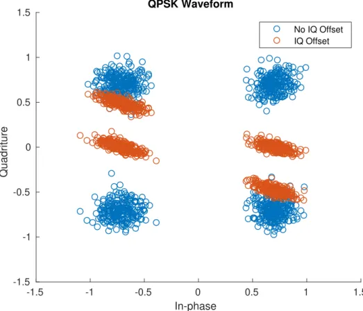
Figure 2.1). The in-phase (top) and quadrature (bottom) signals may not experience the same gains or appropriate phases of 0 and 90 degrees due to manufacturing imperfections or normal wear. . . 26 2.15 An IQ plot (see Appendix A.5) of 1,000 QPSK samples before and after IQ offset (2.31).

Values of φ = 20o,kI = 1, and kQ= 0.7 are used. Notice how the smaller Q gain causes

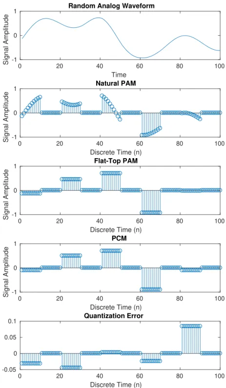
the spread of values to be vertically squeezed on the Quadrature axis. . . 27 2.16 A random analog waveform (see Appendix A.6), its natural Pulse Amplitude

Modula-tion (PAM) waveform obtained through multiplicaModula-tion with an impulse train, its flat-top PAM waveform formed by holding the first value of each pulse, its Pulse Code Mod-ulation (PCM) waveform obtained by quantizing to the nearest value in the codebook [−0.9,−0.7,−0.3,−0.1,0.1,0.3,0.7,0.9], and the residual error resulting from that quan-tization. . . 28 2.17 A section of a time-domain square waveform formulated by summing cosines. While the

states of the square waveform aims to have values of negative and positive one, there are large deviations near high-definition edges, and small ripples in flat sections. If unlucky, these analog deviations can sum to mV values. . . 30 2.18 A periodogram (see Appendix A.2) calculated using a Kaiser window displaying the

non-linear sum of two sinusoids (F1 = 10kHz, F2 = 11kHz). The sum is made non-linear by evaluating each time-domain sample of the sum through the polynomial y = 0.0005x3 + 0.0000001x2+ 0.1x+ 0.003. . . 31 2.19 Two Gaussian pulses (see Appendix A.3) displayed in the frequency domain. If guard bands

(displayed here as 125-175 kHz) are not used or bandwidth (100 kHz in this example) is not carefully allocated, interference can result from neighboring channels (displayed as vertical lines), as shown here.. . . 32 2.20 Class 4 (a) and class 7 (b) industrial noise sequences (see Appendix A.4), each period lasting

1024 samples. This model is reflective of the time-varying nature of industrial noise, as the authors of [32] found different power spectra dominate over others for often periodic time intervals.. . . 33 3.1 A neuron cell (adapted from [2]) is composed of a nucleus which receives signals from many

dendrites. The amount of influence a dendrite has on a neuron is determined by synapses. When the sum of incoming signals is above a threshold, the nucleus fires a signal down its axon, which in turn splits into many dendrites, feeding into other neurons. In this mathematical model inspired by this phenomenon, the previous neurons’ axons carry the signals x0, x1, x2, split into many dendrites. Synapses influence that value by a weight, (w0, w1, w2). The cell body adds weights to each incoming dendrite (b0, b1, b2), computes the dot product of all dendrites, and outputs a signal on its axon defined as the output of some activation functionf whose input is the dot product. . . 36 3.2 An illustration (adapted from [2]) of reducingW ∈[3,4] and b∈[3,1] into a single matrix,

(9)

3.3 An illustration (adapted from [2]) of the computation of class coresf and the resulting loss score Li using both SVM and soft-max functions. Both use the same class scores f, but

have very different interpretations of their results, 1.58 and 1.04. The SVM considers each incorrect score less than a margin below the correct score as a contributor to loss, while the soft-max classifier relays a value proportional to the belief that the label assigned to each signal is correct. . . 39 3.4 An illustration (adapted from [2]) of common data splits between training, validation, and

testing data. In this image, validation is performed on fold 5, training on folds 1-4, and testing on the rest. Next, fold 1 would be used as validation data, and folds 2-5 as training data, and so on, until all 5 folds have been used as the validation data. . . 41 3.5 An illustration (adapted from [2]) of an SVM loss function’s gradient vector (3.9) for a

two-weight linear classifier. Each of the two axis represent values assigned to a weight. In practice, loss functions have pockets of local minima/maxima, and cannot be visualized due to the number of dimensions required to represent each weight used. The color gradient red represents high loss, while blue low loss. The white circle represents the current values chosen for weightswo, w1, the arrow the gradients unit vector, and the dashed line an extension of

that vector. Updating the weights by too much will put the weights (currently green loss) in perhaps a higher loss section of the graph (yellow or red), but adjusting the weights by too little each update will be computationally expensive and perhaps get the SGD stuck in a local minimum of the SVM loss function. . . 42 3.6 The in-phase components of one positive and one negative QPSK symbol, up-sampled to 16

SPS by a Raised-Root Cosine (RRC) filter with a roll-off coefficient of 0.35. Making up half the values of an example flattened training signal vectorxi, classification decisions of a linear

classifier using this signal would likely depend most heavily on samples surrounding the 60th and 80th sample, as they most strongly correlate to what bits are being transmitted. As a result, weights corresponding to those samples would likely be pushed to higher values during SGD. . . 43 3.7 A circuit model (adapted from [2]) showing the forward pass (green) by applying inputs to

the gates operators and backward pass (red) by applying the chain rule recursively. Gates represent a few local operations done by a linear classifier’s neurons. Gates can do both passes totally independent of other gates, without knowledge of the full circuit, or classifier structure. . . 46 3.8 A circuit model (adapted from [2]) showing the forward pass (green) by applying inputs

to the gates operators and backward pass (red) by applying the chain rule recursively of a circuit featuring a ReLU max gate. The blacked out w weight would cause all gates before it to have a gradient of zero, killing those neurons. Using (3.9), the back pass value for w

can be shown to bew= 1×_δaδ2a× _δrδ(r+p)×_δwδ max(w, z) = 1×2×1×0 = 0 . . . 48 3.9 A three-layer neural network (adapted from [2]) with two fully-connected hidden layers. Each

hidden layer has four neurons, and the input has three samples. As shown in Section 3.2, not all architectures use fully connected layers, and for good reason. . . 51 3.10 A comparable CNN (adapted from [2]) to the linear classifier in Figure 3.9. Convolutional

layers are three-dimensional, and only the last few layers are fully connected. The rest of the CNN is much more sparsely connected in an effort to reduce over-fitting and computational cost. . . 52 3.11 Two convolution computations (adapted from [2]) applied to an input (blue) of sizeW = 5,

filters (red) of size F = 3, zero-padding (gray) P = 1, and stride S = 2. Through (3.29), we obtain the output matrix (green) height/width (5−3 + 2×1)/2 + 1 = 3 of depth two due to using two filters for an output shape ∈ [3,3,2]. Highlighted is the computation of

o[2,0,0] = 3, computed as x[4 : 6,0 : 2,0]~w0[:,:,0] +x[4 : 6,0 : 2,1]~w0[:,:,1] +x[4 : 6,0 : 2,2]~w0[:,:,2] +b0[:,:,0] = 3. . . 53

(10)

3.12 Max pooling (adapted from [2]) of a 244 by 244 pixel image. Input size W = 224, filter size

F = 2, and a strideS= 2 resuls in an output shape (3.29) of (224−2 + 2×0)/2 + 1 = 112. Depth is maintained. . . 54 3.13 A ConvNet [3] architecture that passes raw image data through three convolutional layers,

a fully connected dense layer, a maxout layer, and a softmax classifier. . . 54 3.14 An illustration (adapted from [2]) of full-connected neurons before (a) and after (b)

connec-tions are dropped. Arrows represent connecconnec-tions between neurons, while neurons with x’s through them represent neuron connections terminated by being dropped out. . . 57 3.15 A diagram (a) of a simple non-linear neural net with a two neuron hidden layer and a plot

(b) describing its output over values 0< X <1 (see Appendix A.7). . . 59 3.16 A diagram (a) of a ten neuron hidden layer and a plot (b) of their summed output. With each

additional neuron in the hidden layer, the sum of sigmoids at the neuron in the subsequent layer (see Appendix A.7) is a closer approximation of a given continuous waveform. . . 59 3.17 An illustration (adapted from [55]) of three time iterations of (3.30). The black line is the

estimated objective or loss functionf, while the dashed black line is the truef (unknown but visualized). The acquisition function α is in green, whose maxima are highlighted with red arrows, indicating either exploration (when uncertainty σ(·), blue, is large) or exploitation (model prediction is high, solid and dashed black lines match). Observationsxn are marked

as black dots, with the new observations in the n = 3 and n = 4 sub-figures highlighted in red. Notice how new observations reduce uncertainty, and are first taken at high value points (right skewed) to maximize impact on acquisition function reduction. . . 61 3.18 A flow diagram (adapted from [58]) of a GAN testing process (training stage is complete).

Synthetic data samples are formed by the generator via a noise source, and the discrim-inator tries to correctly classify them as fake while classifying real data samples as real. Discriminator average accuracy is bounded by 50% (guessing) and 100% (always correct). Depending on the learning capacity of each neural network and the methods of training, evaluation-time accuracy can fall anywhere in-between.. . . 64 3.19 A flow diagram (adapted from [58]) describing the SGD (3.9) training feedback loop between

the generator and discriminator (used to drive the testing stage shown in Figure 3.18). Parameter updates continue until the learning capacity of the networks are reached and average classification accuracy of the discriminator converge to a steady state value ∈(0.5,1). 65 3.20 A flow diagram (adapted from [60]) describing the various transforms fx, gx, h, fy, gy and

spaces X, Z, Y, C and their interactions at the highest level in domain adaptation. The field is motivated by scarcity of annotated real pictures, but has much wider applications. Implemented correctly, training of classifiers becomes highly generalizable, making testing well under conditions not trained under becomes very robust when domain adaptation is performed on a set of unlabeled data from the new target domain. . . 66 3.21 A set of QPSK constellation points (3.49) forEs = 4. The horizontal axis is defined asφ1(t)

or the real valued element in a complex tuple, and the vertical axis as φ2(t), traditionally represented as the imaginary valued element in a complex tuple. The resulting transforma-tions are n = 1 :b → (0,0) : s→ (2/√2,2/√2), n = 2 : b → (0,1) : s → (−2/√2,2/√2),

n= 3 :b→(1,0) :s→(−2/√2,−2/√2), andn= 4 :b→(1,1) :s→(2/√2,−2/√2) . . . . 69 3.22 A flow chart (adapted from [4]) describing the forward pass (see Figure 3.8) of a set of eight

input values through the CLDNN. A [1,8] input vector is concatenated with values filtered through a [1,8] filter in both the first and second convolutional layer. Each filter (see Figure 11a of [4]) contains eight weights and one bias value (see Figure 3.11 for example filters), which are calculated during SGD (3.9). The Long Short-Term Memory (LSTM) cell holds the values for the soft-max classification layer.. . . 70

(11)

3.23 A 3D modulation classification accuracy plot obtained by testing a range of frequency offset RML2016.10a [5] data samples on a poorly-designed CNN over a range of SNR values. This shows the accuracy floor of 1/11, which indicates the CNN guessing one of the eleven mod-ulation schemes in the dataset due to overwhelming frequency error. The peak accuracy of 35% is quite low due to poor hyper-parameter tuning and a low learning capacity archi-tecture (caused by too much or not enough dropout, filter layers not correctly extracting features, not enough neurons in dense layers, etc). Modulation accuracy spikes at certain periodic values of frequency offset, perhaps due to aliasing (so much spinning that the IQ data doesn’t look like its spinning anymore). . . 71 3.24 A confusion matrix obtained from a constant CFO (2.30) line drawn down the CFO axis

of Figure 3.23 at 13% CFO normalized to sampling rate. The color gradient communicates classification accuracy averaged over SNR values ranging from -20 dB to 20dB. The horizon-tal axis displays the modulation scheme that the CNN classifies signals by, and the vertical axis the ground truth of those signals. A perfectly performing classifier would have a deep blue diagonal matrix, where each signal of each modulation type of each SNR is correctly classified by having the highest soft-max value at its index corresponding to the signals’ ground truth label. . . 72 4.1 Illustration of the proposed framework and the ChannelPush.py script. SampBasic.hdf5

acts as the Dataset Under Test (DUT) while ChannelConfig.ini as the instructions file. SampOut.hdf5 files are written as outputs. The 3D matrix is formed by the instructions file, containing the 2D matrix’s (see Table 4.1) instance variables. The 2D matrix objects are formed by run-time channel class imports. 1D channel sequences (see Figure 4.2) are formed by permuting the channel imperfection objects from the 2D matrix, and the DUT is pushed sample by sample through each sequence in parallel. . . 76 4.2 Example set of eight 1D channel sequences (refer to Figure 4.1) formed by permuting through

the 2D channel object matrix. SampBasic.hdf5 is the DUT, and is pushed through each sequence sample by sample, leveraging Multiprocessing. . . 79 4.3 1 SPS pulse shaped Quadrature Phase-Shift Keying (QPSK) IQ data representing the

base-band data of an Ettus Research N210 transmission. For the sake of visualization, frequency offset from Local Oscillator (LO) drift has been left out. The top track displays the dataset influenced by phase ambiguity and AWGN, then the matched filtering of that data. The bottom track additionally shows STO, where the data is interpolated and filtered up to an intermediate 2 SPS, offset in time, then decimated (and once again match filtered like the top track). . . 82 4.4 The AWGN channel effect is described by its SNR and Gaussian RV variance, σ. Three

AWGN channels of varying SNR but constant σdescribed by ChannelConfig.ini are applied to the same infile sampBasicmod.py. The outputs of which are manually moved to Interme-diate Frequency (IF) folders corresponding to a secondary instructions file, MergeConfig.ini. Merge datasets.py (see Figure 4.5) modulates and sums the independent transmissions. . . 83 4.5 Three 16 SPS pulse shaped QPSK datasets from Figure 4.4 are modulated to intermediate

frequencies 10, 15, and 20 MHz. Each dataset was pushed through the framework as a DUT and modified by a unique AWGN channel block independently, each representing a transmitted signal. Future work will implement this feature to produce MIMO and OFDM datasets. . . 84

(12)

4.6 RML2016.10A is composed of 1,000 training sets containing 128 samples each per class per SNR value. Transmissions average 28.3 bits divergence from theory. The proposed application (see Figure 4.3) averages 36.2 bit divergence from theory. In order to achieve similar KLD entropy at an RF NNs evaluation time to state-of-the-art datasets, this analysis shows the proposed application requires at least 256 samples per transmission. The resulting divergence from theory is 25 bits, or a 11.58% decrease from RML2016.10A. . . 85 5.1 An overview of the DRCNss domain mappings and the space each domain occupies. See

(5.2) to see how they’re used in the DRCNs objective function. . . 88 5.2 The DRCN (adapted from [6]) is composed of two sections: the Convnet [3] classification

NN (left) and reconstruction Convae [6] NN (right). The classification NN performs source label prediction and is composed of three convolutional layers of depth (number of filters)

nb = [100,150,200] where filter size is 3×3. Each max pooling layer condenses a 2×1

grid of values into one equal to the largest of the four. Dropout probability ρ = 0.5, dense layers have 1024 neurons, and the soft-max classification layer has 11 outputs, one for each modulation scheme. The reconstruction NN is an auto-encoder that performs data reconstruction. This teaches commonalities between classifying in both domains, helping the formation of F, transforming to a characteristic-agnostic domain.. . . 89 5.3 Convnet and DRCN training accuracies at each epoch of SGD. The legend indicates whether

(13)

List of Tables

4.1 Example 2D Channel Object Matrix (refer to Figure 4.1). Objects are instances of run-time imported Carrier Frequency Offset (CFO) and Additive White Gaussian Noise (AWGN) Python classes. Instance variables of the objects are imported from the 3D characteristics matrix. Some characteristic sweeps should be linearly spaced (phase ambiguity in radians), and others log spaced (SNR of an AWGN model) . . . 78 4.2 Examples of variations in computer vision image datasets, and a collection of analogies for

their signal domain parallel [2]. . . 80 5.1 A summary describing the statistical differences between the source domain and target

domain datasets. Maximum Doppler frequency is denoted asfD, multi-path taps are defined

by their time delay τ and amplitudea, Nsin describes the number of sinusoids used in the

frequency-selective fading model,FS is the sampling frequency of the simulated transmitter

and receiver, ∆maxt and ∆maxf are the maximum symbol rate and carrier frequency offsets,

σt and σf are the standard deviations of the Gaussian-distributed symbol rate and carrier

frequency offsets, andK is the Rician K-factor ratio of specular to diffuse power. . . 90 5.2 At each stage of training the Convnet classifier is evaluated against a 20% testing partition.

The peak testing accuracy obtained over 30 epochs is presented below for each of the four experiments. . . 92

(14)

List of Acronyms

AC Alternating Current

ACM Adaptive Coding and Modulation ADC Analog to Digital Converter AI Artificial Intelligence

AWGN Additive White Gaussian Noise BER Bit Error Rate

BPF Band-Pass Filter

BPSK Binary Phase Shift Keying BW Band Width

CDF Cumulative Density Function CFO Carrier Frequency Offset

CLDNN Convolutional Long Short Term Deep Neural Network CLT Central Limit Theorem

CMBR Cosmic Microwave Background Radiation CNN Convolutional Neural Network

CPU Central Processing Unit DAC Digital to Analog Converter DC Direct Current

DPD Digital Pre-Distortion

DRCN Deep Reconstruction-Classification Network DUT Dataset Under Test

ECC Error Control Coding FET Field Effect Transistor

(15)

GAN Generative Adversarial Networks GBN Ghost Batch Normalization GPU Graphics Processing Unit GRC GNU Radio Companion IF Intermediate Frequency IIR Infinite Impulse Response IQ In-phase Quadriture

KLD Kullback-Leibler Divergence LNA Low-Noise Amplifier

LO Local Oscillator LOS Line Of Sight

LSTM Long Short Term Memory MAC Medium Access Control ML Machine Learning

MIMO Multiple Input Multiple Output NF Noise Figure

NN Neural Network

OFDM Orthogonal Frequency-Division Multiplexing OLOS Obstructed Line Of Sight

OTA Over The Air

PAM Pulse Amplitude Modulation PCA Principal Component Analysis PCM Pulse Code Modulation PDF Probability Density Function

(16)

QAM Quadrature Amplitude Modulation QPSK Quadrature Phase Shift Keying RCS Radar Cross Section

ReLU Rectified Linear Unit RF Radio Frequency

RFFE Radio Frequency Front End RL Reinforced Learning

RMS Root Mean Square RRC Raised Root Cosine RV Random Variable

SDR Software Defined Radio SGD Stochastic Gradient Descent SNR Signal to Noise Ratio

SPS Samples Per Symbol STO Symbol Timing Offset SVM Support Vector Machine

USRP Universal Software Radio Peripheral

(17)

Chapter 1 Introduction

1.1 Motivation

Since the late 1990s, the use of Neural Networks (NNs) in wireless communications has gained a signif-icant following [7]. In an effort to reduce long analysis and design cycles, as well as improve performance in certain aspects of wireless communications, NNs have been implemented as a data-driven approach to solving many challenges. They have been proven to be an effective approach due to several attractive properties, including adaptive processing, universal approximation, and computational efficiency [8].

With numerous existing closed-form solutions in the field of communications, it may be difficult to know when it is appropriate to use a NN to complete a task. To start, for NNs in wireless communications to be suitable for the challenge under consideration, there must not be a direct, closed-form solution. After it is decided the use of a NN is suitable, it must be decided if the whole problem should be solved using a NN, or just to solve for a portion of the ultimate answer by leveraging a NN. The accuracy of NNs depends first on the quality and relevance of training data to testing data, so whether simulating or experimentally collecting the data, it is important to take care and consider its quality and relevance. Another consideration when implementing NNs is that they can very quickly become computationally burdensome if their architecture is large. Additionally, over-training NNs to noise in the data can present issues when decisions are made by the NN on testing data, and is caused by too many neural connections [7].

1.2 State of the Art

At present, there exist many opportunities for applying data-driven Artificial Intelligence (AI) to com-munications tasks. Digital Pre-Distortion [9] (DPD), localization [10], modulation classification [11], Error Control Code (ECC) decoding [12], Multiple Input Multiple Output (MIMO) detection [13], entire transmit and receive chains [14], Software-Defined Radios [15] (SDRs), and channel modeling [16] have all witnessed

(18)

improvements due to recent advances in AI. The focus of this thesis, however, is in generalized training and testing, and so three of this years most impactful papers on this topic are discussed:

• Deepsig’s 2018 dataset [17] aims to increase machine-learning based signal classification accuracy in the presence of unforeseen noise. A highly-plausible set of noise is synthesized and applied to signals paired with 24 modulation class labels (including high-order modulation schemes such as QAM256). Each signal is additionally paired with a Signal to Noise Ratio (SNR) value ranging from -20 to +20 (a total of 239,616 across all class combinations). A signal contains 1024 complex-valued samples double-precision floating-point values. Each transmission is affected by the non-idealities of Rayleigh fading (taps defined as H , P

iδ(t−Rayleighi(τ)) where τ = [0,0.5,1,2]), carrier

frequency offset ∆fc∼N(0, σclk), pulse shaping using Root-Raised Cosine (RRC) filters with roll-off

values α ∼U(0.1,0.4), phase ambiguity θc ∼ U(0,2π), sampling frequency offset ∆fs ∼ U(0, σclk),

and timing offset ∆t ∼ U(0,16). Using an Ettus Lab B210 Universal Software Radio Peripheral

(USRP), the authors found that a NN trained with their simulated 2018 dataset only suffered a 7% peak modulation classification accuracy penalty compared to the same NN trained with a measured Over The Air (OTA) dataset.

• Researchers from the Israel Institute of Technology [18] investigated the cause of what they call the “generalization gap”, or the phenomenon where NNs trained using mini-batch SGD have a testing accuracy less generalizable to unforeseen noise the bigger the mini-batch size. They found that the generalization gap is caused by having few parameter updates and not from the mini-batches being large. Furthermore, the generalization gap can be reduced by adjusting the training method to include more parameter updates such thatη∝√M, whereηis the parameter update rate and should be increased by a rate proportional to the square root of the mini-batch size,√M. They also showed that weight updates during NN training should be scaled by a unit-mean Gaussian Random Variable (RV) of variance σ2 ∝ M such that local minima in the objective function can be escaped, and the absolute minimum can be reached (thus achieving maximum signal classification performance). Notably, with this method of gradient update noise, the authors did not find much benefit in also implementing the very popular dropout, drop-connect, or label noise, which have been the industry standard for almost a decade. Finally, they present a “Ghost Batch Normalization” method which performs SGD with few parameter updates yet with a insignificant generalization gap. By calculating the mean µl_B_s of thelth batch and standard deviation σl_B_s of small (significantly smaller than batch sizeBL) “Ghost Mini-Batches”, generalization error can be significantly reduced without increasing

η by shifting and scaling the weights γ during SGD by updating in the form γX l₋_µl

Bs

σl Bs

+β where β

(19)

the learning rate needs to be adjusted from standard SGD such that ηL=

q_|

BL|

|Bs|ηs.

• Researchers from Google Brain found that the generalization of a NN corresponds to an “input-output Jacobian norm” and “number of transitions” metrics [19]. Consider the JacobianJ(x) =δfσ(x)/δxT,

where the NN inputs x are passed through the soft-max function fσ, resulting in the generalization

sensitivity metric “Jacobian norm”: Extest

h

||J(xtest)||F

i

around the points of interest xtest. The

second generalization sensitivity metric they define is the number of transitions, or the number of activated ReLU functions (f(x) =max(0, x)) in the hidden layers of a NN. They define this metric as

Extest[t(xtest)], where t(x) =

R z∈T(x) δc_δdz(z)

1dz. Neurons are sampled and put into the space T(x),

and the last hidden layer’s output is described as c(x). The authors plot generalization sensitivity described by those two metrics between inter-class and intra-class perturbations, revealing where in high-dimensional feature-space that perturbations are likely to cause incorrect classification. The paper gives the example of a Gaussian perturbation ∆x∼N(0, I) resulting in a change at the NN’s output equal to ||J(x)||2

F and to the number of transitions equal to t(xtest). If the change at the

output is large enough, incorrect classification occurs.

1.3 Current Issues

A number of issues remain open in the field of machine learning communications [20]. In order to facilitate ML in systems, current wireless network infrastructures need to be updated to deploy Graphics Processing Units (GPUs) at network edges, allowing for computationally efficient use of ML-based solu-tions. Network slicing, or the allocation of wireless network resources for different use cases, is an area of communications that still has seen very little attention from recent advances in AI. Additionally, standard-ized datasets and environments for fair comparisons between architectures still do not exist. While some are more popular than others, there is still not a set of renowned datasets in the wireless community as there is in the computer vision community. Also, there is a significant lacking of theory behind hyper-parameter optimization and data generalization, where both of these tasks are mostly performed by iterating through every option in processes such as hyper-parameter validation, which is a very time consuming process. Distillation or transfer learning is a technique that has not yet been successfully implemented in wireless communications either, or transferring training results from one NN to another for use in a task similar to the first. Although a defensive application was discovered in [21], novel attacks on NNs have shown that the technique became obsolete within months of its writing [22].

Below, issues concerning the three state-of-the-art papers on generalized training are discussed: • Deepsig’s 2018 dataset [17] shows a significant increase in size over their 2016 dataset, going from

(20)

220,000 transmissions of 128 samples to 239,616 transmissions of 1024 samples, or 225.28 MB of double-precision (64-bit) complex values to 1.96 GB. While still a small memory allocation com-pared to many computer vision datasets, generating larger datasets with fewer assumptions increases training time and complexity. It would be valuable for datasets to cover a large range of statistical behaviors using very few samples, a task made difficult given the law of large numbers. Addition-ally, the authors note that matching channel models to real-world deployment conditions is difficult, taking time to estimate and implement to simulate training signals, leaving NNs inoperable for long down-periods.

• Israel Institute of Technology’s GBN method [18] is powerful, however their results show that they can only limit generalization error, at best, to as low as small batch SGD can (but more often reaches an error in-between small and large batch SGD). It would be valuable to navigate around that limit by leveraging a new training method other than small-batch SGD or by manipulating training datasets. • While the development of the Jacobian norm and number of transitions matrices in [19] are powerful metrics in finding the weak points of classifiers, the metrics are not very intuitive to interpret and analyze, and there currently exists no convex-optimization solution to manipulating sensitivity to minimize incorrect classifications. It is difficult to know how to act on how the Jacobian norm and number of transitions to improve peak accuracy.

1.4 Thesis Contributions

This work contains the following contributions:

• A survey of wireless channel environments was given in Chapter2 that can be used in the proposed framework for dataset generation.

• A survey of machine-learning based signal classification was given in Chapter 3 that can be used to implement an unsupervised domain adaptation architecture from Chapter5.

• A framework for wireless transmission dataset synthesis, implementing arbitrary channel environ-ments and baseband waveforms.

• A dataset generated using the framework from Section4was proposed, and was shown to be properly sized, having 11% lower entropy than state-of-the-art datasets.

• A Deep Reconstruction-Classification Network (DRCN) was proposed in Chapter 5, which attempts to maintain peak classification accuracy despite heavy data bias resulting in a 16% peak testing

(21)

accuracy drop compared to an experiment with all else equal but no data bias. These contributions show both data-side (pre-training) and testing-phase manipulations to increase NN generalization and avoid retraining.

1.5 Thesis Organization

The thesis is organized as follows: Chapter2will give a survey of background knowledge learned by the author on the topics of wireless channel modeling. Chapter3surveys neural networks with an emphasis on training and data sets, and modulation classification. Chapter4presents the author’s work on generalized training through the development and use of a low bias, low decay framework that synthesizes low-entropy data sets modeling state-of-the-art wave-forms. Finally, Chapter 5 present’s the author’s ongoing work on generalized training through the use of the domain adaptation technique, and concluding thoughts are discussed in Chapter6.

1.6 List of Related Publications

The following publications resulted from the activities of this thesis research:

• K. McClintick, A. Wyglinski. “Physical Layer Neural Network Framework for Training Data Forma-tion.”IEEE 88th Vehicular Technology Conference, Fall 2018.

• K. Gill, K. McClintick, N. Kanthasamy, “Experimental Test-Bed for Bumblebee-Inspired Channel Selection in an Ad-hoc Network.”IEEE 88th Vehicular Technology Conference, Fall 2018.

(22)

Chapter 2 Understanding the Wireless

Communications Environment

The contributions of this thesis require a systematic understanding of wireless environments. Conse-quently, this chapter presents a survey of classical channel model theory to provide context and knowledge needed in discussion of Chapter 3, dataset synthesis.

Although transmitted waveforms begin as well defined, man-made, synthetic structures, a virtually endless number of probabilistic, and sometimes non-linear, phenomenon alter the observed waveforms receive-side [5]. Even within a single noise model, there can exist a limitless number of variations of that imperfection from one wireless channel to another. Some of the most prevalent and common imperfections include:

1. Additive White Gaussian Noise (Section 2.1), a model used to mimic the effects of many wideband noise sources

2. Path loss (Section 2.2) reduction of signal power density due to reflection (Section 2.3), diffraction (Section2.4), scattering (Section2.5), absorption, aperture-medium coupling loss, and free-space loss 3. Doppler shifts (Section 2.6) resulting from motion of the transmitter, receiver, or scatterers and

reflectors within the wireless channel

4. Carrier Frequency Offset (Section2.7.1) of both the transmitter and receiver’s local oscillators, which drive each radio’s mixers

5. Phase ambiguity (Section2.7.2) introduced by the unknown distance between transmitter and receiver 6. Random Symbol Timing Offset (Section 2.7.3) resulting from independently running sample clocks

(23)

7. IQ imbalance (Section 2.7.4) resulting from phase and magnitude mismatches between the sine and cosine sections of receiver and transmitter chains

8. Rounding of sampled voltages and digital filter coefficients due to Quantization (Section 2.7.5) 9. Electronic Noise (Section2.7.6) caused by semi-conductors such as shot and flicker noise

10. Coupled noise (Section 2.8) resulting from inter-modulation, interference from same and adjacent channels, industrial noise, Cosmic and terrestrial events

When a communications transmit-receive pair move information from one point to another, there is a great deal of sequential tasks that are performed by the transmit and receive chains (see Figure 2.1). It is the goal of this section to describe popular models which discuss the impact of imperfections of these tasks, as well as perturbations introduced during the informations journey from sender to receiver, over the wireless channel. The first such model that is often discussed in this field is Additive White Gaussian Noise (AWGN).

(24)

Figure 2.1: A flo w char t of a transmit and receiv e chain of comm unications tasks. Arro ws indicate mo v emen t of in formation from one blo ck to another. The form that information tak es at eac h step is comm unicated through annotations. An tennas are pictur e d as upside-do wn triangles.

(25)

2.1 Additive White Gaussian Noise

As it will become apparent in this section, there is a virtually unending number of types and sources of noise in a wireless channel. The Central Limit Theorem (CLT) states that as independent random variables are summed, their joint distribution approaches a Gaussian probability density function (PDF):

fx(x) = 1 √ 2πσ2e −(x−µ)2 2σ2 _, _(2.1)

whereσis the standard deviation andµthe mean value of the RV, written asN(µ, σ2_{). AWGN is described}

as additive because it is added to any transmission. There exists enough noise sources to approximate the CLT at all frequencies such that the noise has uniform power across the frequency band. This is why AWGN is described as white, an analogy for how white frequencies of optical wavelengths are the sum of all other colors of the visible light frequency band.

AWGN is fundamental in wireless communications because it imposes a performance ceiling for any task, and that idea extends to NNs involved with wireless data. One way of describing this ceiling was presented by Claude Shannon in [23]. The channel capacityC of a wireless channel with power constraint

1

k

Pk

i=1x2i ≤P fork message codewordsx1, x2, ..., xk, is:

C = 1 2log2 1 + P N , (2.2)

whereN is the wireless channel AWGN variance. Codewords make up a codebook, or all possible messages sent. Consider the optical telegraph [24], a mid-1700s invention of the French Chappe brothers. Five brightly colored panels are painted onto a board and hidden by shutters that can be either open (1) or closed (0), conveying 25 = 32 messages, x ∈ {1,0,0,0,0},{0,1,0,0,0}, ...,{1,1,1,1,1}. The larger the number and dimensionality of codewords, the larger the power constraintP, the larger the channel capacity

C.

2.2 Path Loss

When implementing an AWGN channel model, aLink Budget technique can be used to approximate the signal power, which is needed to determine SNR. A link budget is a calculation that determines received powerPr of a wireless transmission as a function of the transmit chain, wireless channel, and receive chain

parameters. According to the Friis formula, the received power can be calculated in dBm as [1]:

Pr =Pt+Gt+Gr+ 20 log10 λ 4πd , (2.3)

wherePtis the transmitted power,Gr, Gtare the receiver and transmit antenna gains,λis the wavelength

(26)

transmission (d > 2D_λ2, d >10D, d >10λ for antenna length D), the signal is narrowband, and antennas are isotropic in the direction of transmission. Notice that power received decreases with both increased frequency and distance.

For high power, long range transmissions of frequencies up to L-band (2000 MHz) from a tall base-station tower to a mobile user, the most popular topographical path loss model to be used in the free space Friis formula defined by equation (2.3) is the Okumara-Hata [25] empirical path loss model, whose behavior was collected in Tokyo, Japan using isotropic antennas, and has seen widespread use [26]. The formula is rated for use up to 100 km and for at least 1 km, and is rated for a base-station height up to 200 m and a mobile receiver height of up to 3 m. Over the years, many measurement campaigns [27] have been conducted to expand the range of distances and frequencies the model can accommodate. The original Okumara model can be described [28] as use of the Friis formula in (2.3) whereLpath is instead:

L50,dB=LF +Amu(f, d)−G(hte)−G(hre)−GAREA, (2.4)

where L50,dB is the 50th percentile (mean) of the propagation loss, LF is the free space propagation loss,

Amu(f, d) is the median attenuation relative to free space (see Figure 3.24 in [28]), G(hte), G(hre) are the

transmitting and receiving antenna gain factors in (2.5), respectively, andGAREA is the gain with respect

to the type of environment (see Figure 3.23 in [28]).

For various antenna heights, the antenna gain factors can be described as [1]:

G(hte) = 20 log ₂₀₀hte , 1000m > hte >30m (2.5a) G(hre) = 10 log h₃re , hre≤3m (2.5b) G(hre) = 20 log h₃re , 10m > hre >3m. (2.5c)

2.3 Reflections and Fading

Instead of link budgets, Ray Tracing Algorithms can be a preferred category of techniques when de-termining signal power, especially in physically smaller wireless channels with well-defined dimensions. A popular ray tracing model for representation of a channel with path loss is the discrete delay channel model [1] (see Figure 2.2). The model behaves differently for narrow and wideband signals.

(27)

Figure 2.2: The discrete delay channel model, adapted from [1]. Inputs each have isolated time delaysτi,

ray powers|βi|2 =A0ai/di, and ray phasesejφi.

A narrowband signal is defined as a transmissions whose bandwidth does not significantly exceed the coherence bandwidth of the channel the signal is traveling through. A received signal is considered significantly wide if the inverse of the channel’s root mean squared (rms) delay spread τrms:

τrms=

q

τ2_{+ (}_τ₎2_, _(2.6)

is five times smaller than the signal’s bandwidth [1]: 5

τrms

< BW. (2.7)

The delay spreadτn _{is defined as:}

τn₌ PL i=1τin|βi|2 PL i=1|βi|2 , (2.8)

where the additional time required for the ithsignal path, or ray, to arrive is τi, and the power of the ith

ray is|βi|2 =A0ai/di. The path distance of theithray isdi, the overall reflection coefficient of theithray

is: ai= Ki X j=1 aij, (2.9)

where aij is one of Ki reflections for the ith ray. A0 = √

P0, the power of the received signal from one

meter away:

P0=PtGrGt(λ/4π)2. (2.10)

If a signal is determined to be narrowband using (2.7), the received power can be formulated as:

Pr =P0 L X i=1 ai di ejφi (2.11)

where the received phase offset φi =−2πdi/λ. Notice how the phase of each ray ejφi has the potential to

add constructively or destructively (see Figure2.3).

The discrete delay channel model (see Figure2.2) behaves differently for wide band signals. A wideband signal in the frequency domain can be shown to be of a short time duration in the time domain [28]. Often

(28)

0 10 20 30 40 50

Xcar (m) where Xrsu = 25

-75 -70 -65 -60 -55 -50 -45 -40 -35 -30 -25

PNB (dB)

First Order Shadow Fading Bluetooth

Figure 2.3: Bluetooth Pr (2.11) observed by a receiver (See Appendix A.1) from a single car over a 50 m

stretch of road, whose reflections correspond to the scenario described in Figure2.4. Significant fluctuations occur frequently due to phase interference.

these bursts of signals are modeled as impulses, δ(t) (typically Gaussian pulses in application). In ideal wideband communications, each path of arrival an impulse makes from transmitter to receiver are isolated. Additionally, since impulse durations are instantaneous compared to time delays τi and do not overlap in

the time domain, the phase offset of each ray does not add constructively or destructively. Consequentially, the received power of a wideband signal can be formulated as [1]:

Pr=P0 L X i=1 ai di = L X i=1 |βi|2, (2.12)

and unlike (2.11), the phase termejφi _{is missing. The result is that wideband path loss does not vary from}

(29)

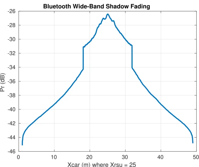
Figure 2.4: Physical Characteristics of the 5-reflection 3D Doppler channel. The paths are attenuated assuming the ground path is dry asphalt[ref] (a5 = 0.34), the roadsides are concrete (a3 = 0.38), and the

cars are metallic (a2,4 = 0.8). The direct path is not attenuated by reflection (a1= 1). Blue-tooth sources

(30)

0 10 20 30 40 50

Xcar (m) where Xrsu = 25

-46 -44 -42 -40 -38 -36 -34 -32 -30 -28 -26

Pr (dB)

Bluetooth Wide-Band Shadow Fading

Figure 2.5: Blue-tooth Pr (2.11) without phase interference observed by a receiver (See Appendix A.1)

from a single car over a 50 m stretch of road, whose reflections correspond to the scenario described in Figure 2.4.

(31)

2.4 Diffractions due to Obstructions

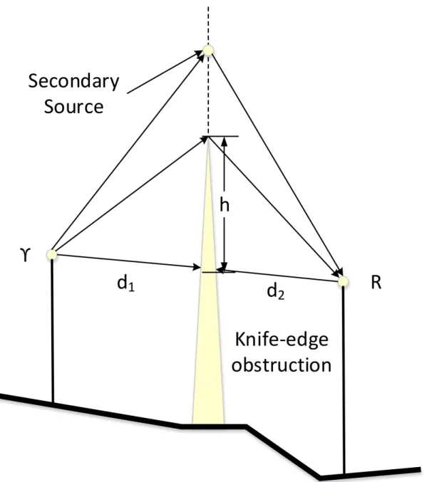
Besides reflections, ray tracing algorithms must consider a phenomenon with electromagnetic waves known as diffraction. Diffraction allows wireless signals to propagate to receivers they do not have Line of Sight to, most notably long range transmissions to receivers blocked by the curvature of the earth. A popular diffraction model used to modify (2.3) is the knife-edge diffraction model [28]. Given the transmitter (see Figure 2.6) Υ receiver R, obstruction of height h above the direct path from Υ to R, and distancesd1, d2 from the transmitter and receiver to the obstruction respectively, the Fresnel-Kirchoff

diffraction parameter can be calculated as:

v=h s

2(d1+d2) λd1d2

, (2.13)

to estimate the additional gain to free space (2.3) as:

GdB = 20 log|F(v)|, (2.14)

where the Fresnel integral can be calculated as:

F(v) = (1 +j) 2

Z ∞

v

e(−jπt2)/2dt. (2.15) While it is often sufficient [28] to model just the largest diffraction, there are situations where a multiple knife-edge diffraction model would increase the accuracy of a path loss model significantly.

2.5 Scattering due to Corrugated Surfaces

The final consideration when determining received power is how electromagnetic waves are scattered. If one is to model path loss given by (2.3) just using the reflection expression of (2.11) and diffraction expression of (2.14), the observed path loss would be higher [28] due to the energy being scattered in all directions when impacting rough surfaces. Surface roughness is described using the Rayleigh criterion [28] defined as the critical height hc in meters:

hc=

λ

8sinθi

, (2.16)

where λ is the signal’s center frequency and θi the signal’s angle of incidence on the flat surface under

consideration. A surface is considered to only have significant scattering if its protuberances are of height greater thanhc. If so, that surfaces reflection coefficientai should be multiplied by a scattering loss factor:

ρ=exp h −8 πσ hsinθi λ 2i I0 h 8 πσ hsinθi λ 2i , (2.17)

(32)

Figure 2.6: An illustration of (2.14), where Υ is the transmitter, R is the receiver, h is the height of the obstruction starting from the direct path from Υ toR, andd1, d2 from the transmitter and receiver to the

obstruction, respectively. The Huygens secondary source mimics a potentially strong reflected path, often taking the form of a reflection off a layer of the earth’s ionosphere.

to formarough =aρs.whereI0 is the Bessel function of the first kind and zero order, andσh is the standard

deviation of the assumed Gaussian variations of the surface’s protuberances about the mean.

A popular link budget model for scattering is the radar cross section model [28], which assumes a large, distant (in the far-field of both the receiver and transmitter, R > 2d_λ2, R >10d, R >10λ), rough surface (defined as h > hc) is scattering a transmission. Like in (2.3), transmit power, antenna gains, and path

(33)

loss are considered, with a few additional terms:

PR(dBm) =PT(dBm) +GT(dBi) + 20log10(λ) +RCS(dB·m2)−

30log10(4π)−20log10(dT)−20log10(dR),

(2.18)

wheredT anddRare the distance from the transmitter and receiver to the scatterer, and the Radar Cross

Section (RCS) can be approximated as the surface area of the scatterer in square meters measured in dB with respect to a one square meter reference.

2.6 Doppler Spectrum

Another wireless phenomenon that can affect system performance is Doppler Shift. In practice, infor-mation is often sent in a radio system under mobile conditions. The impacts of this can be considerable, especially in satellite and railway communications. Consider a sine wave being transmitted via a radio link in a mobile environment, where a transmitter is moving at velocity Vm at an instantaneous distance d0

from a stationary receiver.

As the transmitter moves towards the receiver, the instantaneous distance d0 will shrink, impacting

transmission time as a function of time [1]:

τ(t) =τ0− Vm

c t, (2.19)

where c is the speed of light in free-space, 3·108 m/s, and τ0 = d0/c is the starting transmission time.

Given this, the transmitted sine wave can be formulated by Euler’s formula as [1]:

r(t) =Arej2πfc[t−τ(t)]=Arej[2π(fc+fd)t−φ], (2.20)

where fc is the sine waves carrier frequency, Ar is the amplitude of the received signal, φ = 2πfctau0 is

the current phase offset, andfd is the Doppler shift caused by movement:

fd=

Vm

c fccos(θ), (2.21)

where θ is the direction of movement, for zero degrees being moving straight towards the receiver. The frequency shift observed by the receiver is positive or negative depending on the direction of movement, where magnitude is maximized by the cosine when moving exactly toward or away from the transmitter. Commonly these maximal outcomes of (2.21) are described as the maximum Doppler shift fM =±V_cmfc

of bandwidthBD = 2fM.

However, as shown in Section 2.2, rarely is there one ray (see Figure 2.2) in a wireless channel. Each ray is affected differently, and as consequence the frequency domain representation of the signal is affected by a Doppler spectrum, or Doppler spread D(λ). Consider the wireless channel responding to probing

(34)

impulse responsesδ(t) at time delays τ in the form h(τ, t), where for the inputx(t), the channel output is y(t) =x(t)~h(t): h(τ, t) = L X i=1 βiejφiδ(t−τi). (2.22)

The autocorrelation of the observed impulse response at two different delays and times can then be formu-lated as [1]:

Rhh(τ1, τ2;t1, t2) =Rhh(τ1; ∆t)δ(τ1−τ2), (2.23)

for ∆t=t2−t1. GivenRhh, the autocorrelation in the frequency domain given the time-varying frequency

domain impulse responseH(f;t) =R_−∞∞ h(τ;t)e−jωτdτ is formulated in [1] as:

RHh(f1, f2; ∆t) =RHh(∆f; ∆t), (2.24)

where ∆f = f2 −f1. The channel is assumed to have Wide-Sense Stationary Uncorrelated Scattering

(WSSUS), which is valid for most wireless channels [1]. A WSSUS wireless channel is one in which the delays τi are uncorrelated, and the correlations between paths of equal delays are stationary, or

time-invariant. Given this, the autocorrelation can be estimated asRHh(∆f) if the channel is slowly time-varying

or time-invariant.

Finally, we can derive the Doppler spectrumD(λ) using the Fourier transform of (2.24):

RHH(∆f;λ) = Z ∞ −∞ RHh(∆f; ∆t)e−j2πλ∆td(∆t), (2.25) such that: D(λ) =RHH(0;λ). (2.26)

The spectrum is limited by±fM, and the amount of variation of the spectrum over frequency is described

by the Doppler spread:

B_D,rms2 = RfM −fMλ 2_D₍_λ₎_dλ RfM −fMD(λ)dλ . (2.27)

(35)

Figure 2.7: A flow chart adapted from [1] summarizing equations (2.23) through (2.25). Arrows indicate Fourier (down) and inverse Fourier (up) transforms.

In the most basic multi-path case, (2.26) takes the form:

D(f) = 1 2πfm 1− f fm 2−1/2 ,|f| ≤fm, (2.28)

or Jakes Doppler spectrum, where (2.21) is assumed and can be plotted over normalized frequency as seen in Figure 2.8.

(36)

0 0.005 0.01 0.015 0.02 0.025 0.03 Amplitude

Taps as Beacon Passes Sensor

0.5 1 1.5 2 2.5 3 3.5 4 4.5 5

Tau (seconds) 10-8

(a) Five taps plotted to display phasor delay and magnitude.

-6 -4 -2 0 2 4 6 Frequency w (Hz) 10-10 10-8 10-6 10-4 10-2 100 D (dB) Doppler Spectrum

(b) Jakes Doppler spectrum (b) of the scenario described by Figure2.4.

Figure 2.8: Taps (a) (See Appendix A.1) calculated from the phasers and time delays described by Fig-ure 2.4 as the transmitting car passes by the receiver at x = 25m. Jakes Doppler spectrum (b) where frequency offset is maximal at ±fM (2.21), or movement directly away from and towards the receiver.

Small fluctuations in the spectrum is caused by movement within the channel caused by the leading and lagging vehicles.

However, there is a whole field dedicated to modeling unique cases of Doppler shift. Some common cases in addition to Figure2.8are displayed in Figure 4.9 of [1]. The series of experiments include a series of impulse responses (2.22) and their Fourier transforms, describing a LOS experiment using a stationary radio transmit-receive pair in a stationary environment (BD = 0Hz see (2.27)), and a LOS experiment

using a stationary receiver, but mobile transmitter that moved randomly within a 12 meter radius of a fixed point to simulate a pseudo-stationary mobile user pacing on their telephone (BD = 4.9Hz). An obstructed

LOS (OLOS) experiment is described, using stationary devices 4 meters apart, but with heavy pedestrian traffic around the transmitter (BD = 5.7Hz), and an OLOS experiment with stationary devices, but the

transmitter is rotated at a rate of 2.5 rotations per second (BD = 5.2Hz). Each experiment describes a

family of movement, corresponding to time and frequency domain Doppler signals that can be expected in each, while also showing that BD can be equal for very different spectrum’s D(λ) shapes.

2.7 The Radio Front End

The RFFE (see Figure2.1) is a term used to group all of the analog circuitry between a transmit or receive chain’s antenna and mixer. At the most basic, RFFE’s contain:

• A Band Pass Filter (BPF), used to pass through the expected signal at the expected carrier frequency and block out all other signals and noise. In-band noise and interference is still present. BPFs can also damage signals due to in-band ripple, and are vulnerable to thermal noise, shot noise, and

(37)

transit-time noise (see Section2.7.6).

• A Low-Noise Amplifier (LNA), used to increase the power of in-band signals above the noise floor. LNAs must have a low noise figure (NF), and are often only needed at frequencies above 30 MHz due to the increased path loss (2.3).

• a Mixer, used to combine the carrier waveform with the transmitted or received waveform to form the base-band signal or the Intermediate Frequency (IF) signal.

• A Local Oscillator (LO), used to drive the up-converting and down-converting mixers by creating a carrier cosine waveform. Phase noise (see Section 2.7.6) can be introduced by flicker noise, and the frequency of the carrier can drift with time (see Section2.7.1).

Besides the issues listed above, the initial spacing between a transmit and receive radio can introduce an initial phase offset, introducing phase ambiguity (see Section 2.7.2) even after frequency correction is performed. Digital filters and the DAC/ADC (see Figure 2.1) can introduce significant error to signals through quantization (see Section2.7.5), and in the case of pulse-shaped (see Figure3.6) waveforms, symbol timing offset (STO) (see Section2.7.3) can push bit error rates (BER) to their limits, 1/M (3.48).

Furthermore, the cosine and sine paths of the RFFE (see Figure2.14) experience phase and magnitude imbalances, resulting in stretched IQ plots (see Section2.7.4).

Finally, various forms of electronic noise (see Section2.7.6) can impede SNR, sometimes significantly.

2.7.1 Carrier Frequency Offset due to Local Oscillator Mismatch

Each radio system (see Figure 2.1) has either a down-converter or an up-converter (see Figure 2.9), shifting the center frequency of the signal (see Figure2.10) either up to the carrier frequency if transmitting or down to the base-band if receiving.

However, this frequency shifting is not perfect and is often affected by a phase offset (see Section2.7.6), a frequency offset, and the creation of signal images. Images are lower-amplitude copies ofm(t), the signal being converted by the mixer, appearing at locations:

fimage=      fc+ 2fIF iffLO > fc fc−2fIF iffLO < fc , (2.29a) fimage=fc+ 2fLO, (2.29b)

(38)

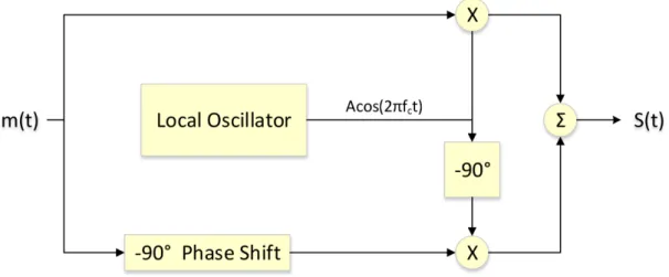
Figure 2.9: An illustration of the base-band signal m(t) being up-converted to the intermediate frequency

fc by a mixer, where the carrier waveform Accos(2π(fc+fo)t) is generated by a local oscillator (LO).

The error introduced by the LO,fo being random and unequal at the transmitter and receiver, frequency

offset is leftover after being down-converted to baseband (see Figure2.10, whether the receiver be a super-heterodyne or direct one.

for down converters and up-converters respectively, where the intermediate frequency fIF = |fc−fLO|.

The frequency offset introduced by LOs can be modeled as [?]:

fo,max=

fc×P P M

106 , (2.30)

where P P M is the parts per million resolution of the LO, often listed in a radio’s user manual,fc is the

carrier frequency, andfo,max is the maximum possible negative or positive frequency offset. For a transmit

receive pair, the total offset can then be defined as fo1 +fo2, where each offset is a Gaussian random

variable bounded by each radio’sfo,max, making the random variable no longer Gaussian. This results in

a minimum possible offset of zero Hertz when each offset is zero (fo1 =fo2 = 0) or equal and opposite to

each other (fo1 =−fo2), and a maximum possible offset of±2×fo,max when the offsets are equal to the

(39)

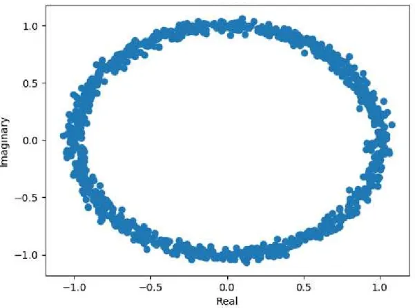
Figure 2.10: An IQ plot of a QPSK message offset in frequency. Phase rotation over time makes demodu-lation inaccurate and Bit Error Rate (BER) high.

2.7.2 Phase Ambiguity after Frequency Correction

As seen in Figure2.3, the received phase offset φi =−2πdi/λcan have significant effects on path loss.

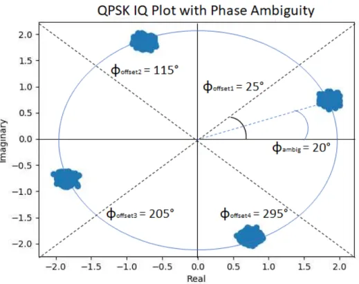
However, this issue goes much deeper than received power: when a demodulator (see Figure2.1) maps a base-band waveform from IQ points to bits, this phase offset rotates the constellation by an amount that has been found experimentally [1] to be random according to the uniform distribution U(0,2π) radians. Consequently, constellation plots such as Figure3.21can become very ambiguous (see Figure2.11), where the plot could be flipped along the real or imaginary axis and still look identical. As a result, various forms of precautions have been developed to avoid errors resulting from phase ambiguity, including equalization, codewords, and differential encoding.

(40)

Figure 2.11: A constellation plot of a QPSK transmission. The four code-words are tilted byφambig = 20◦.

It is the job of a receive chain (see Figure 2.1) to determine if the transmission should be corrected by adding one of the rotations: φof f set1 = 25◦, φof f set2 = 115◦, φof f set3= 205◦, φof f set4= 295◦.

2.7.3 Symbol Timing Offset when Down-Sampling at the Receiver

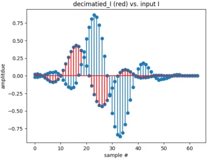
In a radio transmit receive chain (see Figure 2.1), the receiver does not typically have knowledge as to which sample is to be picked to down sample when pulse shaping is implemented (see Figure 2.12). The waveform takes time to transmit, and may be subject to additional delays due to the path taken (see Section2.6). Further, this delay is always changing. As a result, a receiver’s down-sampler must constantly estimate the timing error, filter that error with a loop filter to avoid jerky changes to compensation, and finally apply a correction to the incoming signal.

(41)

(a) Signal without timing error (b) Signal with timing error

Figure 2.12: The in-phase dimension of a pulse-shaped, two symbol (+,-) QPSK transmission (a) and its interpolated, Blackman Harris filtered realization. Additionally, the signal is shifted in time due to a transmission delay this time.

Figure 2.13: A comparison of Figure 2.7.3 (blue) and its time-shifted realization from Figure 2.7.3. The amplitude is reduced due to the amplitudes of a Blackman Harris interpolation filter’s coefficient values.

2.7.4 IQ Imbalance when Modulating

The transmit and receive chains of a radio system (see Figure2.1) contain a similar modulation (see Figure 2.14) and demodulation operations. The magnitude and phase seen by the cosine (in-phase) and sine (quadrature, 90 degrees out of phase) paths of these operations are often not perfectly matched in hardware implementations, resulting in a stretched IQ plot (magnitude imbalance) at the receiver before mapping to bits, or a situation where the I and Q axis are no longer perpendicular due to phase imbalance

(42)

(I is not truly 0 degrees, Q is not truly -90 degrees).

Figure 2.14: An illustration of the in-phase and quadrature paths of the modulator block in a RFFE (see Figure 2.1). The in-phase (top) and quadrature (bottom) signals may not experience the same gains or appropriate phases of 0 and 90 degrees due to manufacturing imperfections or normal wear.

Quality instruments tend to keep this low, although it can vary by large amounts over frequency [29]. IQ imbalance can be modeled at mapping time for each symbol through the expression:

sI =kI×sI0, (2.31a)

sQ=−kQsin(φ)×sI0+kQcos(φ)×sQ0, (2.31b)

where sI0, sQ0 are the balanced in-phase and quadrature components of the symbol, sI, sQ are the IQ imbalanced in-phase and quadrature components of the damaged symbol, kI, kQ are the linear in-phase and quadrature gains, and φ is the phase difference between the two paths. Notice that for φ = 0 and

(43)

-1.5 -1 -0.5 0 0.5 1 1.5 In-phase -1.5 -1 -0.5 0 0.5 1 1.5 Quadriture QPSK Waveform No IQ Offset IQ Offset

Figure 2.15: An IQ plot (see Appendix A.5) of 1,000 QPSK samples before and after IQ offset (2.31). Values of φ = 20o, kI = 1, and kQ= 0.7 are used. Notice how the smaller Q gain causes the spread of

values to be vertically squeezed on the Quadrature axis.

2.7.5 Quantization at Filters and DACs/ADCs

A radio system (see Figure 2.1) experiences numerous forms of discrete approximations of continuous values [30]. Two such examples are the digital approximations of analog waveforms by the ADC, and the floating-point values assigned to derived continuous IIR filter coefficients (16-bit, 32-bit, or 64-bit typically, or 2b discrete amplitudes). While a received waveform has a continuous value, computers only have so much computational power and must reduce the value of voltages and and filter coefficients to discrete values of so many points of precision (see Figure 2.16).