Novel methods for increasing efficiency of quantitative trait locus mapping

(1)

NOVEL METHODS FOR INCREASING EFFICIENCY OF QUANTITATIVE TRAIT LOCUS MAPPING

by

ZHIGANG GUO

M. S., Nanjing Agricultural University, 1998

AN ABSTRACT OF A DISSERTATION

submitted in partial fulfillment of the requirements for the degree of

DOCTOR OF PHILOSOPHY

Department of Plant Pathology College of Agriculture

KANSAS STATE UNIVERSITY Manhattan, Kansas

(2)

Abstract

The aim of quantitative trait locus (QTL) mapping is to identify association between DNA marker genotype and trait phenotype in experimental populations. Many QTL mapping methods have been developed to improve QTL detecting power and estimation of QTL location and effect. Recently, shrinkage Bayesian and penalized maximum-likelihood estimation

approaches have been shown to give increased power and resolution for estimating QTL main or epistatic effect. Here I describe a new method, shrinkage interval mapping, that combines the advantages of these two methods while avoiding the computing load associated with them. Studies based on simulated and real data show that shrinkage interval mapping provides higher resolution for differentiating closely linked QTLs and higher power for identifying QTLs of small effect than conventional interval-mapping methods, with no greater computing time.

A second new method developed in the course of this research toward increasing QTL mapping efficiency is the extension of multi-trait QTL mapping to accommodate incomplete phenotypic data. I describe an EM-based algorithm for exploiting all the phenotypic and

genotypic information contained in the data. This method supports conventional hypothesis tests for QTL main effect, pleiotropy, and QTL-by-environment interaction. Simulations confirm improved QTL detection power and precision of QTL location and effect estimation in comparison with casewise deletion or imputation methods.

(3)

NOVEL METHODS FOR INCREASING EFFICIENCY OF QUANTITATIVE TRAIT LOCUS MAPPING

by

ZHIGANG GUO

M. S., Nanjing Agricultural University, 1998

A DISSERTATION

submitted in partial fulfillment of the requirements for the degree of DOCTOR OF PHILOSOPHY

Department of Plant Pathology College of Agriculture

KANSAS STATE UNIVERSITY Manhattan, Kansas

2007

Approved by: Major Professor James C. Nelson

(4)

Abstract

The aim of quantitative trait locus (QTL) mapping is to identify association between DNA marker genotype and trait phenotype in experimental populations. Many QTL mapping methods have been developed to improve QTL detecting power and estimation of QTL location and effect. Recently, shrinkage Bayesian and penalized maximum-likelihood estimation

approaches have been shown to give increased power and resolution for estimating QTL main or epistatic effect. Here I describe a new method, shrinkage interval mapping, that combines the advantages of these two methods while avoiding the computing load associated with them. Studies based on simulated and real data show that shrinkage interval mapping provides higher resolution for differentiating closely linked QTLs and higher power for identifying QTLs of small effect than conventional interval-mapping methods, with no greater computing time.

A second new method developed in the course of this research toward increasing QTL mapping efficiency is the extension of multi-trait QTL mapping to accommodate incomplete phenotypic data. I describe an EM-based algorithm for exploiting all the phenotypic and

genotypic information contained in the data. This method supports conventional hypothesis tests for QTL main effect, pleiotropy, and QTL-by-environment interaction. Simulations confirm improved QTL detection power and precision of QTL location and effect estimation in comparison with casewise deletion or imputation methods.

(5)

List of Figures

Figure 1.1 Histograms of qualitative and quantitative traits... 11 Figure 1.2 A rice linkage map... 12 Figure 1.3 LOD profiles produced by SM, SIM and CIM methods for QTL mapping... 13 Figure 1.4 Posterior distributions of QTL parameters from Bayesian QTL mapping with

simulated data ... 14 Figure 2.1 Estimated QTL-effect profiles for single-marker, multiple-marker, and shrinkIM

analyses... 26 Figure 2.2 Estimated QTL-effect and LOD profiles for SIM, CIM and shrinkIM... 27 Figure 2.3 3D plots of QTL epistatic effects against chromosome positions for a simulated RIL

population. ... 28 Figure 2.4 3D plots of LOD score of QTL epistasis analysis using 2D IM and shrinkIM... 29 Figure 2.5 The statistical power of QTL detection at three significance levels using SIM, CIM

and shrinkIM... 30 Figure 2.6 LOD profiles produced in the analysis of rice data by SIM, CIM and shrinkIM... 31 Figure 3.1 Statistical power of five multiple-trait QTL-mapping methods with four levels of

missing data. ... 48 Figure 3.2 Power of QTL 1 detection after casewise deletion and by the EM method as a function of the number of complete trait records... 49 Figure 3.3 Means and standard deviations (SDs) of estimates of QTL position by multi-trait QTL analyses... 50 Figure 3.4 Means and standard deviations (SDs) of estimates of QTL effects by multi-trait QTL

analyses... 51 Figure 3.5 LOD profile produced by multiple-imputation method for multi-trait QTL analysis

(7)

List of Tables

Table 2.1 The true values and estimates of QTL parameters in simulation experiment I. ... 32

Table 2.2 Computing time required for SIM, CIM and shrinkIM in simulation experiment I... 33

Table 2.3 QTL parameters used for simulation experiment II... 34

Table 2.4 Estimates of QTL positions and effects for rice data using shrinkIM. ... 35

Table 2.5 Comparison of SIM, CIM and shrinkIM in simulation experiment II... 36

Table 3.1 QTL effects and variances for two traits used for simulation of multi-trait QTL mapping... 53

Table 3.2 Observed statistical power of five multi-trait QTL mapping methods... 54

(8)

Acknowledgements

First, I thank my advisor Dr. James C. Nelson, for his continuous support and access to academic thinking during my doctoral research. He has been a friend and mentor, and has given me inspiration, encouragement and confidence to solve research problems and write scientific papers. Without his support and guidance, I could not have finished this dissertation.

Secondly, I would like to thank my committee members: Drs. Guihua Bai, Haiyan Wang, Shizhong Xu, and outside chair S. Muthukrishnan, for their friendship, good questions,

consideration and encouragement.

Finally, I would like to dedicate this dissertation to my parents Qingen Guo and Cuimei Song, my uncle Qingling Guo and my brother Xiaoqiang Guo. Special thanks go to Xinyan Li, my wife and a caring friend.

(9)

CHAPTER 1 - Quantitative trait locus mapping methods: a review

Quantitative traits have been a major area of genetic studies for over a century(Fisher 1918; Wright 1934; Mather 1949; Falconer 1960). In general, observable traits are of two types: quantitative and qualitative. A quantitative trait such as crop yield and human hypertension shows continuous variation, while a qualitative trait such as eye color shows discrete variation. The expression of a trait is called its phenotype. The phenotype of a qualitative trait is usually determined by a single gene, while the phenotype of a quantitative trait may be determined by many genes and environmental factors. Early studies of quantitative traits were focused on inferring numbers of genes from the mean, variance, and covariance of progenies, with no knowledge of location of the genes that underlie these traits(Kearsey and Farquhar 1997). Recent development of DNA marker technology allows localizing a gene on a chromosome at the DNA level.

To introduce the genetic background for QTL mapping, I begin by reviewing some basic genetic terminology. In eukaryotes, a chromosome is a linear macromolecule composed of DNA. A diploid eukaryotic somatic cell contains multiple pairs of homologous chromosomes.

Homology means similarity by descent from the same ancestral chromosome. For example, corn somatic cells contain 10 pairs of homologous chromosomes. One chromosome of each pair comes from the mother and the other from the father. A parental corn plant produces female or male gametes through a process called meiosis. Each gamete contains a single copy of each chromosome. During meiosis, two homologous chromosomes first physically pair and exchange segments of homologous DNA, resulting in recombination of genes (discussed below) on each chromosome. The paired chromosomes segregate into different cells to form gametes. Male and female gametes fuse to regenerate a plant.

Agene is a unit of inheritance. Each gene is a DNA sequence that carries the genetic information determining the expression of a trait. Within a living cell, genes are arranged in linear order along chromosomes. Each chromosome may contain several thousand genes. The position of a gene on a chromosome is called the locus of the gene. At each locus, variants of the DNA sequence are called alleles. For example, a diploid organism contains two alleles at a locus

(10)

homozygous at the gene locus. Otherwise,the organism is said to be heterozygous. DNA

segmentsused as genetic markers to distinguish different alleles at a given locus are called DNA markers. A DNA marker is not necessarily a gene itself, but it provides genetic information to help identify genes close to this marker on the same chromosome.

The genetic constitution of an individual is called its genotype. For one gene, the

genotype is described by the two alleles at the locus. For example, if there are two alleles A and a at a locus, there are three possible single-locus genotypes AA, Aa and aa in a population. For multiple genes, the genotype is described by a list of the genotypes at all loci. For example, if there are two genes, and each has two alleles, there are nine possible genotypes in a population: AABB, AABb, AAbb, AaBB, AaBb, Aabb, aaBB, aaBb, and aabb.

Genetic recombination generates allele combinations different from those of either parent. Consider two markers on homologous chromosomes. Marker 1 has two alleles A and a, while marker 2 has B and b. Suppose the genotype of P1 is AABB and that of P2 aabb. P1 and P2

produce gametes AB and ab by meiosis. The gametes AB and ab combine to form a F1 progeny

cell with genotype AaBb. By meiosis, a F1 progeny produces four kinds of gametes: AB, ab, Ab

and aB. Among these, AB and ab are parental gametes, and Ab and aB are recombinant gametes carrying alleles from different parents. The ratio of the number of recombinant gametes to the total number of gametes is the recombination fraction between the two loci. Loci with

recombination fraction below 0.5 are said to be linked.

A linear representation of the chromosome with ordered loci is called a linkage map. The unit of a linkage map is the centiMorgan (cM), which is genetic distance calculated based on recombination fraction. If there are many loci on the same chromosome, a linkage map (Fig. 1.2) is constructed by arranging these loci on the chromosome according to the recombination

fractions between all pairs of loci.

A gene locus on a chromosome determining the phenotype of a quantitative trait is called a quantitative trait locus (QTL). QTL mapping is the process of identifying statistical association between the trait phenotype and marker genotype. For QTL mapping, this association is modeled as

(11)

e ~ N(0, σ2).

If there are interactions between different genes, epistasis, these interactions are easily incorporated as covariates into the model.

The first requirement for QTL mapping is making a mapping population. Suppose AA and aa are the genotypes of parents 1 (P1) and 2 (P2) at each locus. Making a cross between P1

and P2 leads to F1 progeny with genotype Aa. Selfing F1 results in F2 progeny with the expected

genotype proportions AA (0.25) : Aa (0.50) : aa (0.25), and continued selfing of progeny for several generations results in recombinant inbred lines (RILs) with the expected genotype proportions AA (0.50) : aa (0.50). Backcrossing the F1 to parent P1 yields BC1 progeny

segregating AA (0.50) : Aa (0.50). These can be backcrossed in turn to give BC2 progeny

segregating AA (0.75) : Aa (0.25). F2, RIL and BC populations are among several types of

QTL-mapping population.

Many statistical methods have been developed for QTL mapping. These methods may be classified into least squares, maximum likelihood, and Bayesian estimation. In the following discussion, the main ideas of these methods are introduced in the historical order of their development. Complex statistical details are omitted for simplicity.

Single-marker tests

Single-marker (SM) includes the t test, ANOVA (ANalysis Of VAriance) or simple regression. The t test and ANOVA focus on testing the difference between phenotypic means of marker genotype classes, while simple regression provides an estimate of marker effect. At a marker, all the progeny is split into distinct groups according to marker genotype and the

phenotypic means of the groups are compared. The t test can be used in populations such as RIL or BC that have only two genotype classes, while ANOVA is used for populations such as F2 that

have three. A marker showing a significant t or F test is presumed to be linked to a QTL. Simple regression for SM is based on the linear model

y = µ + ma + e (1) where y is the phenotype, µ the overall mean of the phenotype, m the genotype of a marker, a the

marker effect, and e residual error following a normal distribution e ~ N(0, σ2).

(12)

Based on this model, unknown parameters µ, a, and σ2 are estimated by the least-squares method,which minimizes the squares of residual errors obtained as the difference between the phenotype and fitted value.

The advantage of SM lies in its simplicity and fast computation. The t test, ANOVA, and simple regression are easily implemented in standard software such as SAS, Splus, R or

MATLAB. However, this method fails to localize a QTL that lies between two markers.

Interval mapping

Simple interval mapping: Simple interval mapping (SIM) (Lander and Botstein 1989) allows localizing a QTL between two markers. Suppose there is a QTL located between markers 1 and 2. At best, SM returns its highest test statistic for the marker closest to the QTL. With SIM, candidate positions at 1- or 2-cM intervals are tested. At a candidate position, if QTL genotype could be observed, simple regression could be used to identify association between phenotype and genotype based on the genetic model

y = µ + za + e (2) where z is the genotype of the putative QTL and a is the QTL effect. However, the QTL

genotype z is unobservable. But its probability distribution conditional on flanking markers may be inferred, and its expectation of z may then be calculated as

) , | 1 ( ) 1 ( ) , | 1 ( ) 1 ( )

(z p z M_left M_right p z M_left M_right

E = + =+ + − =− .

Now a test can be done by the regression of y on E(z) based on model (2). Substitution of

unobserved z with its expectation E(z) increases the variance of the fitted phenotype value by the variance caused by uncertainty of the predicted QTL genotype, leading to reduced test statistics especially at testing positions in wide intervals (Xu 1995).

Better estimates of QTL parameters are obtained by an application of the EM algorithm (Lander and Botstein 1989). EM is a variant of maximum likelihood estimation (MLE),

performed by iteration of expectation (E) and maximization (M) steps. In the E-step, instead of using only flanking markers to infer conditional probability of QTL genotype (prior probability), this method uses both flanking markers and phenotype to infer posterior probability based on

(13)

M steps are repeated until the change in likelihood or parameter estimates is less than a specified value.

The evidence used for the presence of a QTL is LOD (logarithm of odds). It is calculated based on the null hypothesis H0 of no QTL and alternative hypothesis HA of a QTL at the tested

position as

LOD = – log10 (Lreduced / Lfull),

where Lreduced is the log likelihood of the reduced model, corresponding to H0, and Lfull is that of

the full model, corresponding to HA (Lander and Botstein 1989). Repeating this calculation at

every point along a chromosome produces a LOD profile on which peaks indicate the presence of QTLs. Fig. 1.3 shows a LOD profile based on a simulated RIL population.

SIM gives more power for QTL mapping than SM due to exploitation of information from a linkage map (Lander and Botstein 1989, Haley and Knott 1992, Zeng 1994). It allows inferring missing genotype of a marker given its flanking markers. However, SIM considers only one QTL at a time for QTL mapping, and does not model multiple QTLs.

Composite interval mapping: Composite interval mapping (CIM) provides a way to model multiple QTLs (Zeng 1993, 1994; Jansen 1993). The genetic model for CIM is

∑

= + + + = c j i j ij i i z a M b e y 1 μ , (3)

where Mij is the genotype of the cofactor marker j of individual i, and bj the effect of marker j.

The basic idea of CIM is that, when testing for a putative QTL at a testing position, one uses other cofactor markers as covariates to remove variation from these QTLs.

QTL parameters are estimated by the ECM (Expectation/Conditional Maximization) algorithm (Zeng 1993, 1994). ECM is a combination of EM and multiple regression in which the E step is the same as that of EM used by SIM, while the CM step involves estimates of cofactor effects by least squares. ECM produces unbiased estimates of QTL and cofactor effects (Zeng 1993, 1994).

Compared with SIM, CIM provides improved power and precision of estimates of QTL location and effect(Zeng 1993, 1994). However, CIM does not determine automatically the number of cofactor markers to be included in the model. If too many are included, they will overestimate the phenotypic variation caused by background QTLs, reducing the significance of tested QTLs. If too few are included, the advantage of CIM over SIM may be insignificant.

(14)

Moreover, the amount of QTL variation explained by a cofactor marker decreases with increasing genetic distance between the QTL and the marker.

Multi-trait QTL mapping: Multiple-trait composite interval mapping (multi-trait CIM) provides increased power over single-trait mapping by taking into account the correlated

structure of multiple traits (Jiang and Zeng 1995; Korol et al1995, 1998). Correlation between different traits is caused by QTLs controlling the expression of those traits, pleiotropic QTLs. In multi-trait CIM, these traits are assumed to follow a multivariate normal distribution. The

correlation between them is represented by the covariance component in the variance-covariance matrix.

Multi-trait CIM provides formal procedures to test biologically interesting hypotheses concerning the nature of genetic correlation (Jiang and Zeng 1995). These hypothesis tests include QTL main effect, pleiotropy, QTL by environment interaction, and pleiotropy vs. close linkage. However, this method fails to accommodate incomplete phenotypic data. Chapter 3 describes an EM-based algorithm for exploiting all the phenotypic and genotypic information contained in the incomplete phenotypic data.

Multiple-interval mapping: Multiple-interval mapping (MIM) uses multiple marker intervals simultaneously to fit multiple QTLs directly in the model for mapping QTL (Kao et al. 1999). With MIM, a stepwise selection procedure with likelihood ratio test statistic as a criterion is used to identify QTL. The procedure begins with no QTL, and then adds or drops QTL one at a time. In the first QTL analysis, one QTL identified using SIM or CIM is incorporated into the model and used as a cofactor for mapping the next QTL. In the QTL analysis, the intervals with a putative QTL and the QTL identified in the first analysis are tested simultaneously in the model. A stepwise regression procedure is used to determine which QTL should be included or dropped from the model for the next QTL search. This process is repeated until the likelihood ratio test for a putative QTL is lower than a critical value. Thus, for a candidate QTL at a testing position, MIM uses QTLs identified in the previous analyses instead of cofactor markers as covariates to adjust genetic background. For this reason it provides better power and precision of QTL mapping than SIM and CIM.

(15)

Bayesian QTL mapping

Bayesian QTL mapping provides a flexible way to search for multiple QTLs

simultaneously. This method makes inferences about parameters in a way different from MLE or regression-based methods used by SIM or CIM. Based on a probabilistic model with a parameter vector Ф = [θ1, θ2] where θ1, θ1are parameters in the model, the likelihood function L is defined

as the conditional probability of observations given Ф. Formally, L can be written as ) | ( ) ; (Φ Y p Y Φ L = ,

where Y represents a sample from the model. A point estimate of Ф can be obtained by maximizing L with respect to θ1 or θ2. In the Bayesian approach, inference is based on the

posterior probability of Ф. According to Bayes’ Theorem, this is

∑

Φ Φ = = = |) | ( ) ( |) | ( ) ( ) , ( ) , ( ) ( ) , ( ) | ( Φ Y Φ Φ Y Φ Y Φ Y Φ Y Y Φ Y Φ p p p p p p p p p , (4)

wherep(Ф), the prior probability of Ф, quantifies the knowledge we have about θ1 and θ2 prior

to analysis. In general, it is difficult to calculate joint posterior probability p(θ1, θ2|Y) in closed

form from equation (4), but easy to calculate the marginal posterior probability of θ1 or θ2 as

∑

= 1 ) ( ) , | ( ) ( ) , | ( ) , | ( 1 2 1 1 2 1 2 1 θ θ θ θ θ θ θ θ θ p p p p p Y Y Y (5)

given fixed θ2, and

∑

= 2 ) ( ) , | ( ) ( ) , | ( ) , | ( 2 2 1 2 2 1 1 2 θ θ θ θ θ θ θ θ θ p p p p p Y Y Y (6)

given fixed θ1. Sampling Ф from p(Ф| Y) is replaced with drawing θ1 and θ1 in turn from their

marginal posterior probability distributions [equations (5) and (6)]. This strategy is called Gibbs sampling. Continued sampling of this kind is known as the Markov-chain Monte Carlo (MCMC) method, because the previous sample values are used as parameters to sample the next values, generating a Markov chain. Fig. 1.5 gives an example of Bayesian QTL mapping based on simulation.

With Bayesian QTL mapping methods, the most difficult problem is sampling the posterior probability of QTL number. While QTL location and effect are relatively easy to sample, determining QTL number is a problem of model selection (Broman and Speed 2002).

(16)

Models with different number of QTLs are compared, and the best one is selected based on a specific selection criterion such as AIC or BIC. In Bayesian analysis, the optimal model is selected by a probabilistic jump of MCMC from a model with m QTLs to a new one with m + 1 or m – 1 QTLs. Reversible-jump MCMC (RJMCMC) (Green 1995) provides a method for realizing this jump between models with different number of QTLs. RJMCMC has been applied in many Bayesian QTL mapping methods for identifying multiple QTLs (Thomas et al. 1997; Sillanpää and Arjas 1998; Stephens and Fisch 1998; Yi and Xu 2000; Gaffney 2001; Yi and Xu 2002; Yi et al. 2003; Narita and Sasaki 2004). However, it requires much more computation than SIM or CIM, and its convergence is very sensitive to the specification of prior probabilities of parameters.

A recent development in Bayesian QTL mapping, the shrinkage Bayesian method, includes all markers in a model simultaneously in a single test (Xu 2003). When the number of markers is larger than that of individuals, the model is oversaturated. The problem of the oversaturated model is that it cannot provideunique estimates of marker effects. With the shrinkage Bayesian method, the problem is solved by the assumption that the effect of each marker follows a normal distribution with its own mean and variance. The assumption is used to limit large fluctuation of marker effect estimates, and obtain unique estimates. This leads to shrinkage estimates of marker effects, resulting in clear signals of QTL effects. Based on shrinkage estimation, spurious QTL effects are shrunk towards zero, while real QTL effects are estimated with virtually no shrinkage. Penalized MLE (PMLE) (Zhang et al. 2005), an extension of the shrinkage method in MLE, was developed to reduce the computation associated with the shrinkage method and analyze marker-marker interaction. However, PMLE and shrinkage Bayesian mapping are marker-based mapping methods. They cannot be used for interval mapping.

Shrinkage interval mapping (shrinkIM) method (see more details in chapter 2) extends PMLE and shrinkage Bayesian method to interval mapping. It combines the advantages of shrinkage Bayesian method and PMLE. This method allows analyzing QTL and QTL epistasis based on mapping populations.

(17)

References

Broman K. W., and Speed T. P., 2002 A model selection approach for the identification of quantitative trait loci in experimental crosses. Journal of the Royal Statistical Society 64: 641-656

Calinski T., Kaczmarek Z., Krajewski P., Frova C. and Sari-Gorla M., 1999 A multivariate approach to the problem of QTL localization. Heredity 84: 303-310.

Doerge R. W., 2001 Mapping and analysis of quantitative trait loci in experimental populations. Nature Genetics 3:43-52

Falconer D. S. 1960 Introduction to Quantitative Genetics, Oliver and Boyd, Edinburgh. Fisher R. A. 1918 The correlation between relatives on the supposition of Mendelian

inheritance. Philosophical Transactions of the Royal Society of Edinburgh 52: 399-433. Green P. J., 1995 Reversible jump Markov chain Monte Carlo computation and Bayesian model

determination. Biometrika 57: 97–109.

Haley C. S. and Knott S.A., 1992 A simple regression method for mapping quantitative trait loci in line crosses using flanking markers. Heredity 69: 315-324.

Jansen R. C. 1994 Genotype-by-environment interaction in genetic mapping of multiple quantitative trait loci. Theoretical and Applied Genetics 91: 33-37.

Jiang C. J., and Zeng Z. B., 1995 Multiple trait analysis of genetic mapping for quantitative trait loci. Genetics 140: 1111-1127.

Kearsey M. J., Farquhar G. L. F., 1997 QTL analysis in plants; where are we now?. Heredity 80: 137-142

Korol A. B., Ronin Y. I. and Kirzhner V. M.. 1995 Interval mapping of quantitative trait loci employing correlated trait complexes. Genetics 140: 1137-1147.

Korol A. B., Ronin Y. I., Nevo E. and Hayes P. M.. 1998 Multi-interval mapping of correlated trait complexes. Heredity 80: 273-284.

Mather K. 1949 Biometrical Genetics, 1st edition. Methuen, London.

Lander E. S., and Botstein D., 1989 Mapping Mendelian factors underlying quantitative traits using RFLP linkage maps. Genetics 121:185-199.

Sillanpää M. J. and Arjas E., 1998 Bayesian mapping of multiple quantitative trait loci from incomplete inbred line cross data. Genetics 148: 1373-1388.

(18)

Sillanpää M. J. and Arjas E., 1999 Bayesian mapping of multiple quantitative trait loci from incomplete outbred offspring data. Genetics 151: 1605-1619.

Wright S. 1934 An analysis of variability in number of digits in an inbred strain of guinea pigs. Genetics 19:506-536.

Xu S., 1995 A comment on the simple regression method for interval mapping. Genetics 141: 1657-1659.

Xu S., 2003 Estimating polygenic effects using markers of the entire genome. Genetics 163: 789-801.

Zeng Z. B., 1993 Theoretical basis of precision mapping of quantitative trait loci. Proceedings of the National Academy of Sciences USA 90: 10972-10976.

(19)

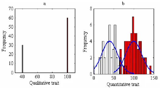
Figure 1.1 Histograms of qualitative and quantitative traits.

Figures a and b show the phenotypic frequency distributions of a qualitative and a quantitative trait in a sample with 100 individuals. In b, the phenotype of a trait was simulated from a normal distribution with mean 40 or 100 and standard deviation 20.

(20)

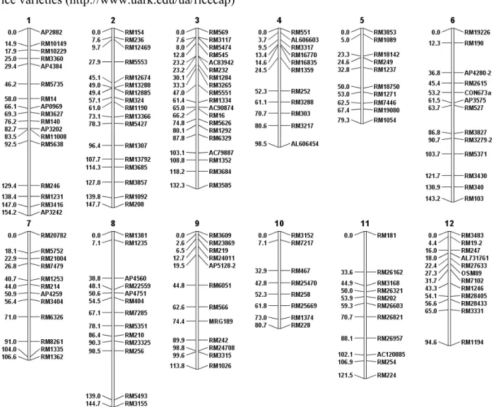
Figure 1.2 A rice linkage map.

The genotypic data used was from a rice QTL study focused on improving grain yield of U.S. rice varieties (http://www.uark.edu/ua/ricecap)

(21)

Figure 1.3 LOD profiles produced by SM, SIM and CIM methods for QTL mapping.

SM: single-marker mapping; EM-based SIM: EM-based simple interval mapping; regression-based SIM: regression-regression-based simple interval mapping; CIM: composite interval mapping. The horizontal black dashed line represents 0.05 significance level LOD threshold 2.17 estimated from 1000 permutation tests with regression-based SIM. The blue dots on the SM curve show effect and location of each marker.

(22)

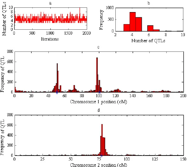
Figure 1.4 Posterior distributions of QTL parameters from Bayesian QTL mapping with simulated data

Posterior frequencies of QTL number and locations were calculated from 2000 MCMC iterations based on a simulated RIL population with 300 individuals. Fig. a: a plot of QTL number over iterations. Fig. b: Posterior frequency of QTL number. Fig. c: posterior frequency of QTL location on chromosome 1. Fig. d: posterior frequency of QTL location on chromosome 2. Asterisks show the true positions of simulated QTLs.

(23)

CHAPTER 2 - Shrinkage interval mapping for QTL and QTL

epistasis analysis in line crosses

Abstract

QTL modeling is an example of an oversaturation problem, requiring the choice of a subset from an excess of explanatory variables. Shrinkage Bayesian and penalized maximum likelihood estimation (PMLE) approaches have been shown to give increased power and resolution for estimating QTL main or epistatic parameters. However, Bayesian methods are computationally expensive and PMLE cannot localize a QTL within an interval. We describe a two-step shrinkage interval-mapping method, shrinkIM, which addresses both weaknesses. In the first step, PMLE is used to select cofactor markers or pairwise marker–marker interactions, reducing the dimensionality of the oversaturated model. In the second step, partially penalized maximum likelihood estimation (PPMLE) is used for QTL interval mapping or QTL epistasis analysis. PPMLE, in which only the parameter of interest — QTL main or epistatic effect — is penalized, provides shrinkage estimates of these effects as well as least-squares estimates of other parameters in the model. Studies based on simulated and real data show that shrinkIM provides higher resolution for differentiating closely linked QTLs and higher power for identifying QTLs of small effect than conventional interval mapping methods, with no greater computing time.

Introduction

Interval-mapping methods for finding a predictive relationship between DNA marker genotypes and quantitative-trait phenotypes fall into three general statistical classes: likelihood maximization by EM algorithm used for simultaneous estimation of genotype and trait

distribution parameters (Lander and Botstein 1989); least-squares estimation by regression of phenotypes on QTL genotype expectations (Haley and Knott 1992); and Bayesian methods. The last approach treats all parameters as random variables and constructs their posterior distributions given priors, using Markov chain Monte Carlo estimation (Satagopan et al. 1996; Sillanpää and

(24)

Arjas 1997, 1999; Yi and Xu 2001; Wang et al. 2005). Various extensions of the first two approaches have been developed for modeling multiple QTL (Zeng 1994), QTL–environment interaction (Jansen 1994), multiple traits (Jiang and Zeng 1995; Hackett et al. 2001; Korol et al. 2001) and multiple interval mapping (Kao et al. 1999). All approaches face the difficult model-selection problem: finding a reduced model to explain the response (phenotype data) in the presence of numbers of explanatory variables (DNA markers) that exceed the number of observational units (individuals) such that there is no unique solution to a full model.

Recent approaches to this problem, while incorporating all the markers, apply shrinkage (Groß, 2003, p. 150) to reduce the effective dimension of the model. Shrinkage methods penalize model coefficients by treating them as drawn from a normal distribution centered on zero,

thereby “shrinking” them toward a prior mean of zero (Boer et al. 2002). Two shrinkage approaches have been suggested: Bayesian and penalized likelihood, the latter including penalized regression such as ridge regression. Typical of shrinkage methods is a QTL profile scan showing a near-zero baseline over most of the genome map, with a few QTL signals standing out conspicuously.

Bayesian shrinkage method: Xu (2003) developed a Bayesian regression method, multiple-marker analysis, for simultaneously estimating the genetic effect associated with the markers along the whole genome map. Each marker effect is allowed to have its own variance parameters so that the variance can be estimated from the data. Wang et al. (2005) extended this method to allow localizing a QTL within an interval, using Metropolis-Hastings sampling since the QTL location parameter does not have an explicit posterior distribution. However, the Bayesian method is time-consuming to compute.

Ridge regression: Consider the linear model Y = Xβ + ε, where Y is a n × 1 trait vector,

X a n × m marker matrix, β a m × 1 vector of regression coefficients, and ε a n × 1 random error vector with ε ~ N(0, Inσ2_{). For an oversaturated model, ordinary least-squares estimates of β}

cannot be calculated as (X’X)-1X’Y because matrix X’X is singular. However, ridge regression can provide a restricted least-squares estimate as (X’X + τIn)-1X’Y under the quadratic

(25)

Penalized maximum-likelihood estimation: The penalized maximum-likelihood estimation (PMLE) method suggested by Zhang and Xu (2005) imposes a prior normal distribution N(μj , σj2) penalty on each βj, allowing the penalty to vary across β. An iterative

algorithm is used to estimate regression coefficients β and other parameters. In essence, PMLE is an extension of the multiple-marker Bayesian method of Xu (2003). However, PMLE can

localize a QTL only to a marker and not between markers.

Shrinkage interval mapping: The foregoing efforts demonstrated that shrinkage estimation methods can provide increased resolution and power as well as low background, but have a few disadvantages. To deal with these we have developed shrinkage interval mapping (shrinkIM), a two-step method. In the first, dimension-reducing step, cofactor markers or marker–marker interactions are selected as suggested by Zhang and Xu (2005) using PMLE, turning the oversaturated model into a regular model. In the second step, a partially penalized maximum likelihood estimation (PPMLE) method — a hybrid of PMLE and least squares — is used to estimate parameters. Instead of penalizing all βs in a model as does PMLE, PPMLE imposes a prior normal-distribution penalty only on the parameter of interest (QTL main or epistatic effect) so that a shrinkage estimate can be obtained. Estimates of other βs are calculated by least squares. In the following description, since PMLE, the method used for cofactor

selection, is identical with Zhang and Xu’s method (2005), we will focus on PPMLE as used in the second step of shrinkIM.

Methods

One-QTL model for shrinkIM: The method described here is based on a RIL

(recombinant inbred line) design but is easily extended to backcross, F2, or other designs. The

linear model for shrinkIM is

∑

= + + + = p j i j ij i i z x c y 1 ε α μ (1)

Here yi is the trait value of individual i; μ is the overall mean; zi is the genotype of a QTL for

individual i; α is the additive effect of the QTL; xij is the genotype of the jth cofactor marker in

the ith individual and is a dummy variable taking the values 1, 0, and -1 for genotypes A1A1,

(26)

genotype zi is not observed and is replaced in the model with its expectation, calculated from the

probability distribution of QTL genotype conditional on the closest flanking markers (Haley and Knott 1992). Missing xij genotype data is similarly imputed.

In this model, the parameter in which we are interested is QTL effect α, while other regression coefficients including overall mean and effects of cofactor markers are treated as nuisance parameters, included only to account for background (polygenic variation). We may combine these and rewrite model (1) in matrix form as

Y = Zα + Xβ + ε (2)

where n is the number of individuals, Y a n × 1 vector of trait values, Z a n × 1 vector of QTL genotype expectations, α the additive effect of the QTL, X a n × (p + 1) matrix with the first column composed of n ones, β a vector of regression coefficients (μ, c1, c2, …, cp)′, and ε ~

N(0, Inσ2_).

To estimate parameters α, β and σ2_{, we introduce partially penalized maximum}

likelihood estimation (PPMLE), a hybrid of penalized maximum likelihood and least squares estimations. Our aim is to obtain shrinkage estimates of parameters of interest in order to realize the advantages associated with shrinkage Bayesian or PMLE, including increased QTL

resolution, high power and low background. First we apply to α the penalty function N(μα, σα2) from PMLE, imposing a normal distribution in order to limit the fluctuation of α. Then we specify the direction of shrinkage of α by placing the second penalty N(0, σα2 /η) on the mean μα of α, where η > 0 denotes a prior sample size (Zhang and Xu 2005). In this way we force α to shrink towards zero. The log likelihood functions for model (1) before and after penalization are

∑

= + + − − = n i j j ij i i z a x c y n L 1 2 2 2 ₍ ₍ ₍ ₎₎ 2 1 ) 2 log( 5 . 0 ) log( μ σ πσ (3) and 2 2 2 2 1 2 2 2 ) 2 log( 5 . 0 ) ( 1 ) 2 log( 5 . 0 ) ) ( ( 2 1 ) 2 log( 5 . 0 ) log( α α α α μ η σ π μ πσ μ σ πσ − − − − − + + − − − =

∑

= a c x a z y n L n i j j ij i i penalized . (4)

(27)

In practice, an iterative two-step algorithm may be used to estimate the parameters. It starts with initial values for θ(0)_{= (}_α(0)_{, β}(0)_,_σ2(0)_,_μ

α(0), σα2(0)), setting iteration counter k = 0. In step 1, we calculate the least-squares estimate of β given α,

) ( ' ) ' ( 1 ( ) ) 1 (k _X_X _X _Y _Z_a k β + = − − _.

In step 2, estimates of α and hyperparameters μα and σα2 are calculated by maximizing penalized log likelihood function (4) given β as

) ( 2 ) ( 2 ) ( 2 ) ( 2 ) ( ) 1 ( ' ) ( ' k k k k k k a α α α σ σ σ σ μ + + − = + Z Z Xβ Y Z , ) ( )' ( 1 ( ) ( ) ( ) ( ) ) 1 ( 2 k _a k k _a k k n Y−Z −Xβ Y−Z −Xβ = + σ , 1 ) ( ) 1 ( + = + η α μ_αk k _, ] ) [( 5 . 0 ( ) ( ) 2 2( ) ) 1 ( 2 k k k k α α α α μ ημ σ + = − + _.

Steps 1 and 2 are repeated until norm ||θ(k)_{- θ}(k - 1)_{|| <}_τ_{, where}_τ_{is a given critical value; we}

used 0.00001.

A likelihood ratio test under the null hypothesis H0: α = 0 and the alternative hypothesis

HA: α ≠ 0 is LRT = –2 ln (Lreduced / Lfull), where Lreduced is the log likelihood of the reduced

model, corresponding to the null hypothesis, and Lfull is that of the full model, corresponding to

the alternative hypothesis (Lander and Botstein 1989). Both are calculated from equation (3) and a LOD score is calculated as LRT/(2 ln 10).

QTL epistasis model for shrinkIM: The linear model for pairwise QTL interaction is

∑

= ≠ + + + + + + = p j i q v u iu iv uv j ij rs is ir s is r ir i z z z z x c x x w y 1 ε α α α μ (4)

where αrs is the interaction effect between QTL r and s (r ≠ s) and wuv the interaction effect

between markers u and v (u ≠ v). Now the parameters of interest are αr, αs and αrs, and the other

regression coefficients are treated as nuisance parameters. Model (4) can be rewritten as model (2) and parameters estimated using PPMLE. The hypothesis test for QTL epistasis is H0: αrs = 0

(28)

It will be noted that pairwise interactions may be detected even between QTLs neither of which exerts a main effect.

Simulation studies: The properties of the shrinkIM algorithm were compared with those of conventional interval-mapping methods, based on simulated and real data. The prior value η = 5 was used in the analysis of simulation or real data, but in tests, no difference was found with values of 10 or 20, echoing the finding of Zhang and Xu (2005). The initial values of prior parameters μα and σα2 were set to 0 and 0.1. Power to detect a given QTL was calculated as the proportion of replicates showing a LOD peak above threshold within the interval containing the QTL (Haley and Knott 1992; Jiang and Zeng 1995; Zhang and Xu 2005). All calculations were implemented in MATLAB (The MathWorks, Inc.), a mathematical and statistical computing language.

In each of two simulation experiments, RIL populations of 300 individuals were generated based on a 300-cM chromosome with 31 evenly spaced markers. The model for the simulation is

∑

= = + = QTL nEPI k in im mn n j ij j i q q q y 1 1 α α

where yi is the phenotype of individual i, αj is the main effect of QTL, αmn is the epistatic effect

of QTL m and n, nQTL is the number of main effects, nEPI is the number of epistatic effects, qij is

the genotype of QTL j of individual i. Environmental error for yi was sampled from a normal

distribution with mean zero and variance σ2. In both experiments, the calculation interval (step size) used for interval mapping was 1 cM. Cofactors for CIM were selected by forward stepwise regression; those for PMLE by the criterion |bj|/σ > 10-6, where bj is the estimate of effect of

marker j and σ is the estimate of the error standard deviation.

Experiment I: The resolution and background level for the detection of QTL or QTL epistasis in a single simulated population were examined. A RIL population was simulated according to the QTL parameters given in Table 2.1. Two types of analyses were performed to identify QTL main and epistatic effects respectively.

(29)

regression (SIM) (Haley and Knott 1992), and CIM (Zeng 1994). The based version EM-SIM (Lander and Botstein 1989) was also computed, but since the results were virtually identical to those of SIM, we used this method only for speed comparison. The evidence for the

identification of a QTL was evaluated based on QTL effect and LOD score. The same three cofactor markers were used in both shrinkIM and CIM. We also calculated a variant of the main-effect model that included four marker–marker interaction cofactors calculated by PMLE. In order to test the sensitivity of the estimate of QTL effect to the choice of prior parameters μα and

σα2, we ran a separate set of shrinkIM analyses in which the initial μα and σα2 were varied independently along the respective ranges [–5:5] and [0.1:1] and the means and standard deviations of QTL effect estimates at each point on the map were computed.

Analysis 2: The QTL-epistasis model was used. ShrinkIM was first compared with

PMLE and then with a two-dimensional scan by SIM. In the comparison of shrinkIM and PMLE, only QTL epistatic effect was used as evidence to claim QTL interaction, since a LOD test statistic is not available for PMLE.

Experiment II: We simulated 500 replicates of 300 individuals according to the QTL positions and effects given in Table 2.3. The statistical power, accuracy, and precision of QTL detection using the same three interval-mapping methods were compared at three significance levels: α = 0.05, 0.01 or 0.001. The LOD threshold for each method was calculated from an additional 2000 simulations with the same total variance of 52.17 but no QTLs.

Analysis of rice data: The phenotypic and genotypic data used for QTL mapping came from a QTL study in rice (http://www.uark.edu/ua/ricecap). A population of 129 RILs from the cross of U.S. rice lines RT0034 x Cypress genotyped at 155 SSR marker loci along a 1500-cM map of 12 chromosomes was used for the detection of QTL affecting days to heading. The mean length of marker intervals was 10.6 cM, with the longest interval 40.5 cM. The population was phenotyped at three locations in Arkansas, Texas and Louisiana with two replicates for each location. Two QTL have been identified from the data of Texas and Louisiana using CIM (results not shown). This prior knowledge was used as a reference for the analysis of Arkansas data. For simplicity, we analyzed only one replicate from Arkansas to illustrate the difference between results from SIM, CIM and shrinkIM. As with the simulated data, we used the same set of cofactor markers for both shrinkIM and CIM.

(30)

Results

Simulation experiment I: Fig. 2.1 shows the more accurate estimation of QTL positions and effects using shrinkIM compared to single-marker or multiple-marker analysis. The

background signal from PMLE or Bayesian based multiple-marker analysis is the same as that of shrinkIM.

Fig. 2.2 shows the increased resolution of shrinkIM of closely linked QTLs 1 and 2 based on QTL effect and on LOD score compared with SIM or CIM. ShrinkIM gave sharper separation than CIM of closely linked QTLs 1 and 2 based on either effect (Fig. 2.2a) or LOD score (Fig. 2.2b) and reduced the background effect to baseline, while SIM was unable to separate the linked QTLs and consistently overestimated QTL and background effects (Figs. 2.2a). For this

simulated dataset, the inclusion of marker–marker interactions as cofactors made no appreciable difference to the results.

Table 2.2 shows comparison of computing times used for 1000 permutations in SIM, SIM, CIM, and shrinkIM in analysis 1, showing that shrinkIM is faster than CIM and EM-SIM. We attribute this to the fewer iterations required in the PPMLE step.

QTL effect estimates proved to be very insensitive to variation in initial values for hyperparameters μα and σα2. Their standard deviation across at least ten values was less than 10-5, negligible in comparison with the estimated effect size of ~3.

Fig. 2.3 shows 3D plots of QTL epistatic effect against chromosome positions; not visible is a spurious close double peak produced by the PMLE method. As with main QTL effects, shrinkIM is expected to provide more accurate estimates of positions of QTL interactions than PMLE, since the latter is limited to testing marker positions, while shrinkIM can localize QTL at any position on the genetic map. Table 2.1 compares position and effect estimates from shrinkIM with those of PMLE for the detection of QTL main and epistatic effect. The background signal of shrinkIM is comparable to that of PMLE (Fig. 2.3a). 2D SIM was not able to identify QTL-QTL interaction based on only QTL-QTL epistatic effect due to strong background, whereas shrinkIM clearly identified three QTL epistatic effects.

(31)

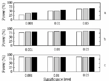
Experiment II: For the detection of QTL 1 and 2 with higher heritability compared to QTL 3, the power of SIM, CIM and shrinkIM was similar. Fig. 2.5 shows the increased power of shrinkIM for the detection of QTL 3 with relatively lower heritability compared with SIM or CIM. The accuracy and precision of estimates of QTL effects and positions are very close for CIM and shrinkIM (Table 2.4).

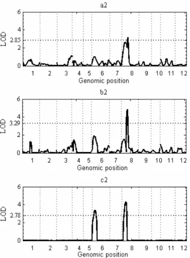
Analysis of rice data: Fig. 2.6 shows the increased power of shrinkIM for the detection of the QTL on chromosome 6 based on QTL effect or LOD score. In SIM and CIM analysis, the QTL on chromosome 8 was identified, but neither method found the second one, a QTL

expressed strongly in the other growing locations and possibly representing Hd6a, a QTL identified near the rice Waxy locus in several other crosses. Position and effect estimates for the two QTL are given in Table 2.5.

Discussion

We have shown the advantages of shrinkIM over conventional SIM and CIM in the detection and identification of QTL or QTL epistasis. ShrinkIM offered higher resolution of closely linked QTL, greater power to identify QTL and more accurate estimates of QTL

parameters without increased cost in execution time. The improved statistical properties are due to the control of polygenic background by two steps. The first step is similar to CIM except for the use of PMLE for the selection of cofactors for markers or interactions between markers, which accounts for the genetic variance due to QTL or QTL epistasis elsewhere in the genome. The additional power of shrinkIM is conferred by the reduction of background toward zero in the case of no QTL at a map position.

More than an extension of PMLE from marker-based mapping to interval mapping, shrinkIM inherits the advantages of shrinkage Bayesian, PMLE and penalized regression.

Though a variant of PMLE, PPMLE offers two apparent improvements on PMLE. First, it limits penalization to parameters of interest in order to obtain shrinkage estimation, while exploiting the simplicity of least squares. Second, it eases the dependence of parameter estimates on the prior parameters in PMLE by decreasing the number of penalized parameters in the model.

As a hybrid of shrinkage estimation and least squares, PPMLE is readily extended to handle multi-environment data if the factor effects are treated as fixed. It can also be used for the discovery of genotype-by-environment interaction or for combined analysis based on families

(32)

from multiple crosses. If collinearity of factors of a genetic model is problematic, we suggest replacing with ridge regression the ordinary least-squares estimate in the first step of PPMLE. As with other regression-based interval mapping methods, parameter estimates are subject to some bias in case of sparse marker maps. This is easily remedied by incorporation of the EM

algorithm, in which the probability distribution of QTL genotypes is posterior-updated using the flanking markers and phenotype.

The clean background produced by shrinkIM results from shrinkage estimation of QTL main or epistatic effect. It is reasonable to ask whether QTLs of small effect can be excluded by shrinkage of these effects to zero in the whole-genome scan. Wang et al. (2005) showed that the Bayesian shrinkage method could detect a QTL accounting for 2% of phenotypic variance, while Zhang and Xu (2005) showed that PMLE could detect a QTL epistatic effect accounting for only 0.5%. In our simulation shrinkIM detected QTL accounting for 6% phenotypic variance. In practice, the power of shrinkIM may approximate to those of the Bayesian shrinkage method and PMLE because of the similar penalty distribution used in these methods. Further simulation studies should resolve the question.

ShrinkIM combines themerits of the other QTL mapping methods we have considered, in being able to identify QTL or QTL epistasis based on either QTL effect or LOD score. Though shrinkage Bayesian method and PMLE show excellent performance for the detection of QTL or QTL interactions from their effect estimates, the absence of test statistics for the tested QTL remains a problem to apply these methods(Wang et al. 2005). In contrast, for conventional interval mapping such as SIM and CIM, LOD is commonly used as evidence to claim a QTL, but the QTL effect profile cannot be used for this purpose because of noisy background. Like the Bayesian approach, shrinkIM supplies QTL evidence by sharpening the QTL effect profile.

The method proposed here may be extended to ECM-based QTL mapping. ShrinkIM is a combination of shrinkage and least squares estimates. Regression-based QTL mapping, though easier to implement and faster to compute, gives biased parameter estimates with sparse markers (Xu 1995) or when QTLs interact or are closely linked (Kao 2001). If we include posterior probability f QTL genotype given flanking markers and observation in step 1 of our algorithm,

(33)

References

Boer M. P., Braak C. J. F. and Jansen R. C., 2002 A penalized likelihood method for mapping epistatic quantitative trait loci with one-dimensional genome searches. Genetics 163: 951-960.

Churchill G. A. and Doerge R. W., 1994 Empirical threshold values for quantitative trait mapping. Genetics 138: 963-971.

Groß J. 2003. Linear Regression. Springer, Berlin.

Hackett C. A., Meyer R. C. and Thomas W. T. B., 2001 Multi-trait QTL mapping in barley using multivariate regression. Genetic Research 77: 95-106.

Haley C. S., and Knott S. A., 1992 A simple regression method for mapping quantitative trait loci in line crosses using flanking markers. Heredity 69:315-324.

Jansen R. C. 1994 Genotype-by-environment interaction in genetic mapping of multiple quantitative trait loci. Theoretical and Applied Genetics 91: 33-37.

Jiang C., and Zeng Z. B, 1995 Multiple trait analysis of genetic mapping for quantitative trait loci. Genetics 140: 1111-1127.

Korol A. B., Ronin Y. I., Itskovich A. M., Peng J. and Nevo E., 2001 Enhanced efficiency of quantitative trait loci mapping analysis based on multivariate complexes of quantitative traits. Genetics 157:1789-1803.

Lander E. S., and Botstein D., 1989 Mapping Mendelian factors underlying quantitative traits using RFLP linkage maps. Genetics 121:185-199.

Satagopan, J. M., Yandell B. S., Newton M.A. and Osborn T. G., 1996 A Bayesian approach to detect quantitative trait loci using Markov chain Monte Carlo. Genetics 144: 805–816. Wang H., Zhang Y. M., Li X., Masinde G. L., Xu S., 2005 Bayesian shrinkage estimation of

QTL parameters. Genetics 170: 465-480.

Xu S., 2003 Estimating polygenic effects using markers of the entire genome. Genetics 163: 789-801.

Yi N. J., and Xu S., 2000 Bayesian mapping of quantitative trait loci under complicated mating designs. Genetics 157: 1759-1771.

Zeng Z. B., 1994 Precision mapping of quantitative trait loci. Genetics 136: 1457-1468.

(34)

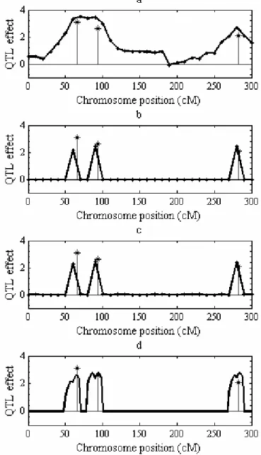
Figure 2.1 Estimated QTL-effect profiles for single-marker, multiple-marker, and shrinkIM analyses.

a: single-marker; b: multiple-marker using PMLE; c: multiple-marker Bayesian; d: shrinkIM. Asterisks show the true positions and effects of simulated QTL.

(35)

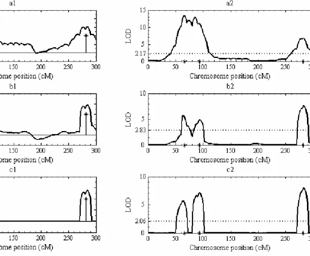
Figure 2.2 Estimated QTL-effect and LOD profiles for SIM, CIM and shrinkIM.

a: SIM; b: CIM; c: shrinkIM. Asterisks show the true positions of simulated QTL in a2, b2, c2 and their effects in a1, b1, c1. The horizontal dotted lines represent the empirical p = 0.05 LOD thresholds from 1000 permutations.

(36)

Figure 2.3 3D plots of QTL epistatic effects against chromosome positions for a simulated RIL population.

(37)

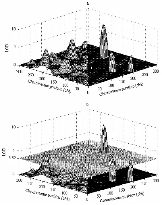
Figure 2.4 3D plots of LOD score of QTL epistasis analysis using 2D IM and shrinkIM.

In a and b, the left-hand side of the figure shows 2D IM and the right-hand side shrinkIM. In b, the horizontal surface at LOD 3.39 represents the threshold calculated for 2D IM from 1000 permutations, giving a conservative comparison since the calculated threshold for QTL epistasis analysis using shrinkIM was actually 3.13.

(38)

Figure 2.5 The statistical power of QTL detection at three significance levelsusing SIM, CIM and shrinkIM.

(39)

Figure 2.6 LOD profiles produced in the analysis of rice data by SIM, CIM and shrinkIM.

a: SIM; b: CIM; c: shrinkIM. The horizontal dotted lines in the right-hand plots represent empirical LOD thresholds for the three methods, calculated at significance level 0.05 from 1000 permutation tests. Horizontal axes are on cM scale; labels indicate rice chromosomes.

(40)

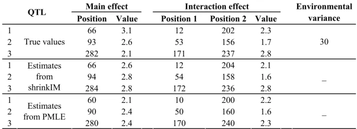
Table 2.1 The true values and estimates of QTL parameters in simulation experiment I.

Positions are in cM.

Main effect Interaction effect QTL

Position Value Position 1 Position 2 Value

Environmental variance 1 66 3.1 12 202 2.3 2 93 2.6 53 156 1.7 3 True values 282 2.1 171 237 2.8 30 1 66 2.6 12 204 2.1 2 94 2.8 54 158 1.6 3 Estimates from shrinkIM _{284 2.8} ₁₇₂ ₂₃₆ _2.8 _ 1 60 2.1 10 200 2.2 2 90 2.4 50 160 1.6 3 Estimates from PMLE 280 2.4 170 240 2.3 _

(41)

Table 2.2 Computing time required for SIM, CIM and shrinkIM in simulation experiment I

Computing time was evaluated from 1000 permutations for SIM, CIM and shrinkIM. The computer used has a 2-GHz CPU; times are expected to scale similarly on a faster machine

Method Computing time (sec)

SIM 32 EM-SIM 697

CIM 855 shrinkIM 348

(42)

Table 2.3 QTL parameters used for simulation experiment II. Positions are in cM. QTL Position Additive effect Genetic variance Proportion Total variance 1 56 1.7 2.89 0.06 2 153 2.4 5.76 0.11 3 282 3.1 9.61 0.18 Total 18.26 0.35 52.17

(43)

Table 2.4 Estimates of QTL positions and effects for rice data using shrinkIM.

Positions are in cM.

QTL Chromosome Position QTL effect R2

1 8 36 3.57 0.13

(44)

Table 2.5 Comparison of SIM, CIM and shrinkIM in simulation experiment II. Positions are in cM. QTL 1 QTL 2 QTL 3 Significance Level Method LOD threshold Power (%) Position SD Effect SD Power (%) Position SD Effect SD Power (%) Position SD Effect SD SIM 2.1 63.2 56.0 2.4 1.96 0.39 82.0 153.3 2.00 2.55 0.41 87.2 282.3 1.71 3.15 0.40 CIM 2.7 64.6 55.9 2.5 1.86 0.32 85.6 153.3 1.92 2.45 0.37 85.8 282.2 1.62 3.10 0.38 0.05 shrinkIM 2.0 65.8 55.8 2.6 1.62 0.34 86.0 153.3 1.96 2.27 0.43 85.4 282.2 1.55 2.94 0.40 SIM 2.9 51.6 55.9 2.4 2.07 0.35 82.0 153.2 2.00 2.56 0.41 87.2 282.3 1.71 3.15 0.40 CIM 3.7 52.2 56.0 2.4 1.95 0.29 85.0 153.3 1.92 2.45 0.37 85.8 282.2 1.62 3.10 0.38 0.01 shrinkIM 2.9 56.0 55.9 2.6 1.71 0.30 84.8 153.3 1.87 2.30 0.39 85.2 282.2 1.65 2.94 0.40 SIM 4.3 28.6 56.0 2.1 2.30 0.29 78.2 153.2 1.99 2.59 0.38 87.0 282.2 1.70 3.15 0.39 CIM 4.6 37.8 55.8 2.3 2.06 0.21 83.2 153.3 1.91 2.47 0.36 85.8 282.2 1.55 3.10 0.38 0.001 shrinkIM 4.1 41.8 55.9 2.4 1.84 0.25 82.9 153.3 1.87 2.30 0.39 85.2 282.2 1.64 2.95 0.38

(45)

CHAPTER 3 - Multiple-trait quantitative trait locus mapping with

incomplete phenotypic data

Abstract

Conventional multiple-trait quantitative trait locus (QTL) mapping methods must discard cases (individuals) with incomplete phenotypic data, thereby sacrificing other phenotypic and genotypic information contained in the discarded cases. Under standard assumptions about the missing-data mechanism, it is possible to exploit these cases. We present an EM-based algorithm that supports conventional hypothesis tests for QTL main effect, pleiotropy, and

QTL-by-environment interaction. Simulations confirm improved QTL detection power and precision of QTL location and effect estimation in comparison with case deletion or imputation methods. The EM method may be incorporated into any least-squares or likelihood-maximization

QTL-mapping approach.

Introduction

Statistical methods for identifying and mapping genes controlling complex traits, commonly known as quantitative trait loci or QTL, have been developed to a high degree. The primary focus has been on methods for single traits (Lander and Botstein1989; Haley and Knott 1992; Jansen 1993; Zeng 1994; Satagopan et al. 1996; Kao and Zeng 1999; Yi and Xu 2003; Wang et al. 2005; and many others). It was proposed (Jiang and Zeng 1995; Korol et al. 1995) that QTL mapping methods that consider simultaneously several correlated phenotypic traits, or a single trait measured in several environments, offer increased detection power and precision of location and effect estimation over single-trait QTL mapping. This is because trait-by-trait QTL-searching neglects information contained in the data about the common influence of a QTL on more than one trait or in more than one environment. With the promise of increased power from a multivariate approach comes an interesting problem: what to do when some of the multivariate data are missing.

(46)

Two main statistical approaches have been elaborated for multi-trait QTL analysis: regression (Korol et al. 1995, 1998; Calinski et al. 1999; Knott and Haley 2000; Hackett et al. 2001) and maximum likelihood or ML (Jiang and Zeng 1995). Regression QTL-mapping

methods, though easier to implement and faster to compute, give biased parameter estimates with sparse markers (Xu 1995) or when QTLs interact or are closely linked (Kao 2001), while ML methods are free of these defects (Kao 2001). It has also been proposed to transform multiple traits into canonical variates so that conventional univariate interval QTL mapping can be applied (Weller et al. 1996; Mangin et al. 1998; Calinski et al. 2000), but interpretation of the results may be difficult.

Though QTL-mapping data are often incomplete, information-recovery methods are at present applied only to genotypic data. For incompletely informative marker-genotype data, posterior distributions are readily estimated from flanking markers in the same individual (Jiang and Zeng 1997). For unknown QTL genotypes at tested positions in map intervals, maximum-likelihood (ML) methods estimate posterior distributions simultaneously with the parameters of a phenotypic mixture distribution (Lander and Botstein 1989), while regression methods (Haley and Knott 1992) replace missing QTL genotypes with their expectations given flanking markers. Variations based on sampling include multiple imputation as described by Sen and Churchill (2001) and Bayesian approaches (e.g. Satagopan et al. 1996; Sillanpää and Arjas 1998, 1999; Yi and Xu 2001; Wang et al. 2005).

In contrast to genotypic data, missing phenotypic data for any trait results in discarding all cases (individuals) lacking even one value, sacrificing all other phenotypic and genotypic information available for these cases. The problem was recognized by Knott and Haley (2000), but they provided no solution. Is there an alternative to this “casewise” (Allison 2002) deletion?

Methods for completion of incomplete multivariate data are of two kinds: by imputation (single or multiple) and by EM algorithm. Single imputation typically replaces missing data with three kinds of values: a value drawn from a specific model-based distribution, a mean calculated from other observations of the same variable, or a conditional mean calculated by least-squares regression on predictors. Multiple imputation (Rubin 1987, 1996) fills in missing data multiple

(47)

maximization of the likelihood over both original and imputed data. In contrast, the EM

algorithm as described by Dempster et al. (1977) focuses not on replacing a missing value with its expectation, but on using the information available in the original dataset. In the framework of EM, missing data imputed are in effect integrated out of the complete-data log likelihood by iterative refinement of their expectation. Little and Rubin (2001) provided an EM algorithm for incomplete multivariate data, and extended it to accommodate multiple regression with missing responses.

Here we describe an adaptation of Little and Rubin’s EM method (2001) to the case of multi-trait QTL mapping with incomplete phenotypic data. We show that the tests for QTL main effects may be constructed as in Jiang and Zeng (1995), and we describe the properties and behavior of the test statistics and QTL effect and position estimates based on simulation studies.

Methods

Missing-data mechanism is ignored: Several kinds of “missingness” have been defined (Rubin 1976). Here we consider only MAR, “missing at random”, meaning for our purposes that the probability of missing phenotypic data within any genotype class is unrelated to the

phenotypic value. Either for MAR or the stronger assumption, MCAR or “missing completely at random” (missingness also independent of genotype), estimation methods need not model a missing-data mechanism.

Multivariate regression with incomplete data: Consider the linear model

m n m p p n m n× =X × B × +E × Y , (1)

where Y is a (n × m) response matrix with n the number of individuals and m the number of traits (or environments); X is a (n × p) design matrix with p predictors; E is an error matrix and Ei (i =

1, 2, …, n) follows a multivariate normal distribution with means zero and variance–covariance matrix ⎟ ⎟ ⎟ ⎟ ⎟ ⎠ ⎞ ⎜ ⎜ ⎜ ⎜ ⎜ ⎝ ⎛ = 2 2 2 2 1 2 2 2 22 2 21 2 1 2 12 2 11 mm m m m m σ σ σ σ σ σ σ σ σ L M O M M L L V (2)

Suppose there are some missing entries in Yi (i = 1, 2, …, n). Now matrices Yi,

B X

(48)

] , [ miss i obs i i y y Y = , (3) ] , [ miss i obs i i μ μ μ = , (4) ⎥ ⎦ ⎤ ⎢ ⎣ ⎡ = ) ( ), ( ) ( ), ( ) ( ), ( ) ( ), ( i miss i miss i obs i miss i miss i obs i obs i obs V V V V V . (5)

For a random sample with n individuals, the log likelihood of observations is given by

∑

= − = − − − − − = n i obs i obs i i obs obs i obs i n i i obs obs nm 1 1 , T 1 , ( ) ( ) 2 1 ln 2 1 ) 2 ln( 2 ) ; , (B V Y π V y X B V y X B l (6)

Since in general, it is difficult to calculate the MLEs of parameters directly by maximizing (6) with respect to the individual parameters, we may adapt Little and Rubin’s EM (2001) algorithm to obtain the MLEs of parameters in model (1) as follows.

ALGORITHM 1: Starting with initial values_θˆ(0) ₌[_Bˆ(0),_μˆ(0),_Vˆ(0)]_{, iterate the following} two steps until convergence.

E step: ) ( 1 ) ( ) 1 ( ) 1 ( ) ( ) 1 ( _, ₎ _ˆ ₍ _ˆ ₎ˆ ˆ ( obsk k k i obs i k miss i k obs i k miss i obs i obs i miss i obs i E y + y θ =μ + + y −μ + V_y _y V_y− _y , (7) ) , ( ( 1) ) 1 ( + ₌ missk+ i obs i k i y y y . (8) M step: ) 1 ( T 1 T ) 1 ( ₍ ₎ ˆ k+ ₌ _X _X − _X _Y k+ B , (9) ) 1 ( ) 1 ( ˆ ˆ k+ ₌_X_B k+ μ , (10) n k k k k k ( ˆ ) ( ˆ ) ˆ( +1) ₌ Y( +1)−μ( +1) T Y( +1)−μ( +1) V (11)

Multi-trait QTL mapping with incomplete phenotypic data by regression: We now describe our multi-trait QTL mapping method with incomplete data. Though the method given is based on a recombinant inbred line (RIL) population, it is easily extended to other mating

designs such as F2 or BC. The statistical model for multiple-trait analysis (Jiang and Zeng 1995,

Korol et al. 1995, Hackett et al. 2001) based on complete phenotypic data is +

+

=z a x b E