Convolutional neural networks for malware classification

(1)

Convolutional Neural Networks for

Malware Classification

Daniel Gibert

Director: Javier Bejar Department of Computer Science

A thesis presented for the degree of Master in Artificial Intelligence

Facultat d’Informàtica de Barcelona (FIB) Facultat de Matemàtiques (UB)

Escola Tècnica Superior d’Enginyeria (URV)

Escola Politècnica de Catalunya (UPC) - BarcelonaTech Universitat de Barcelona (UB)

Universitat Rovira i Virgili (URV)

(2)

Abstract

According to AV vendors malicious software has been growing exponentially last years. One of the main reasons for these high volumes is that in order to evade detection, malware authors started using polymorphic and meta-morphic techniques. As a result, traditional signature-based approaches to detect malware are being insufficient against new malware and the catego-rization of malware samples had become essential to know the basis of the behavior of malware and to fight back cybercriminals.

During the last decade, solutions that fight against malicious software had begun using machine learning approaches. Unfortunately, there are few open-source datasets available for the academic community. One of the biggest datasets available was released last year in a competition hosted on Kag-gle with data provided by Microsoft for the Big Data Innovators Gathering (BIG 2015). This thesis presents two novel and scalable approaches using Convolutional Neural Networks (CNNs) to assign malware to its correspond-ing family. On one hand, the first approach makes use of CNNs to learn a feature hierarchy to discriminate among samples of malware represented as gray-scale images. On the other hand, the second approach uses the CNN architecture introduced by Yoon Kim [12] to classify malware samples accord-ing their x86 instructions. The proposed methods achieved an improvement of 93.86% and 98,56% with respect to the equal probability benchmark.

(3)

Acknowledgments

I would first like to thank my family, especially Mom, for the continuous support she has given me throughout my time in graduate school. Second, I would like to express my gratitude to my supervisor, Dr. Javier Béjar for their guidance during the course of this thesis.

(4)

List of Figures

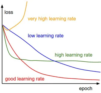
2.1 Effects of different learning rates . . . 18

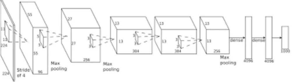
2.2 AlexNet architecture . . . 21

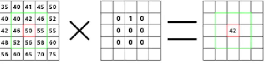
2.3 Convolution . . . 22

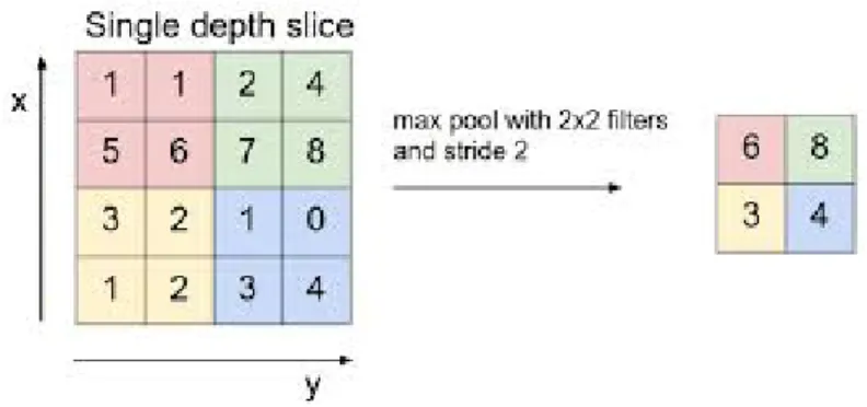
2.4 Max pooling . . . 23

2.5 ReL and sigmoid functions comparison . . . 29

3.1 Most frequent 14 opcodes for goodware . . . 34

3.2 Most frequent 14 opcodes for malware . . . 34

3.3 Outline of Invencea’s Malware Detection Framework . . . 36

3.4 Visualizing Malware as an Image . . . 38

4.1 Malware Classification Challenge: dataset . . . 40

4.2 Snapshot of one bytes file . . . 41

4.3 Snapshot of one assembly code file . . . 42

4.4 Top 10 opcodes in the training dataset . . . 44

4.5 Average of opcodes per malware family . . . 44

5.1 Visualizing Malware as a Gray-Scale Image . . . 54

5.2 Rammit samples . . . 55

5.3 Lollipop samples . . . 55

5.4 Kelihos_ver3 samples . . . 56

5.5 Vundo samples . . . 56

(8)

LIST OF FIGURES 5.7 Tracur samples . . . 57 5.8 Kelihos_ver1 samples . . . 57 5.9 Obfuscator.DCY samples . . . 57 5.10 Gatak samples . . . 58 5.11 Shallow Approach . . . 59 5.12 Overview architecture A: 1C 1D . . . 62 5.13 Overview architecture B: 2C 1D . . . 64 5.14 Overview architecture C: 3C 2D . . . 66

5.15 Approach A: CNNs training results . . . 68

6.1 Yoon Kim model architecture . . . 73

6.2 Skip-gram model architecture . . . 75

6.3 t-SNE representation of the word embeddings . . . 78

6.4 CNN Embedding layer output . . . 80

6.5 CNN Convolutional layer output . . . 81

6.6 CNN Max-pooling & output layer . . . 82

6.7 Heuristic Search: Learning Rate . . . 84

6.8 Heuristic Search: Embedding size . . . 84

6.9 Heuristic Search: #Filters . . . 85

6.10 Heuristic Search: Filter Sizes . . . 86

(9)

List of Tables

4.1 Number of samples per class with 0 instructions . . . 45 4.2 Winner’s solution: confusion matrix . . . 47 4.3 List of feature categories and their evaluation in XGBoost . . 49 5.1 CNN 1C 1D: confusion matrix . . . 68 5.2 CNN 2C 1D: confusion matrix . . . 69 5.3 CNN 3C 2D: confusion matrix . . . 69 6.1 CNN without pretrained word embeddings: confusion matrix . 87 6.2 CNN with pretrained word embeddings: confusion matrix . . . 88 6.3 Approach B: Test scores . . . 88

(10)

Chapter 1 Introduction

Malware, short for malicious software, refers to software programs designed to damage or do any kind of unwanted actions on a computer system such as disrupting computer operations, gather sensitive information, bypass access controls, gain access to private computer systems and display unwanted ad-vertising. Malware can be divided into the following categories not mutually exclusive depending on their purpose.

• Adware. It is a type of malware that automatically delivers adver-tisements. Advertising-supported software often comes bundled with software and applications and most of them serve as a revenue tool. • Spyware. It is a type of malware that spies and track user activity

with-out their knowledge. The capabilities of spyware can include keystrokes collection, financial data harvesting or activity monitoring.

• Virus. A virus is a type of malicious software capable of copying itself and spreading to other computers. Viruses can spread through email attachments, through the network the computer is connected if any other computer inside the network has been infected, by downloading software from malicious sites, etc.

(11)

• Worm. It is a type of malware that they spread through the computer network by exploiting operation system vulnerabilties. The major dif-ference between worms and viruses is that computer worms have the ability to self-replicate and spread independently while viruses rely on human activity to spread.

• Trojan. A Trojan horse is a type of malware that disguises itself as a normal file or program to trick users into downloading and in-stalling malware. A trojan can give unauthorized access to the infected computer and be used to steal data (logins, financial data, even elec-tronic money), install more malware, modify files, monitor user activity (screen watching, keylogging, etc), use the computer in botnets, and anonymize internet activity by the attacker.

• Rootkit. A rootkit is a type of malicious software designed to remotely access or control a computer without being detected by users or security programs. For example, Rootkits can prevent a malicious process from being visible or it can keep its files from being read, etc.

• Backdoors. A backdoor is a computer software designed to bypass normal authentication procedures and compromise the system. Once a system has been compromised, one or more backdoors may be installed in order to allow access in the future without being detected by the user. • Ransomware. It is a type of malicious software that essentially restricts user access to the computer by encrypting the files or locking down the system while demanding a ransom. Users are forced to pay the malware author to remove the restrictions and gain access to their computer. This type of payment is usually done with Bitcoins.

• Command & Control Bot. Bots are software programs created to au-tomatically perform specific operations. Bots are commonly used for

(12)

web spiders or for distributing malware. One way to defend against bots is by using CAPTCHA tests in websites to verify users as human. Nowadays, the detection of malicious software is done mainly with heuristic and signature-based methods that struggle to keep up with malware evolu-tion. Signature-based methods haven been heavily used for antivirus software for decades. A malware signature is an algorithm or hash that uniquely iden-tifies a specific virus. While identifying a particular virus is advantageous it is quicker to detect a virus family through a generic signature. Virus re-searchers found that all viruses in a family share common behaviors and a single generic signature can be created for them. However, malware authors always try to stay a step ahead of AV software by writing polymorphic and metamorphic malware to do not match virus signatures. On one hand, poly-morphic code uses a polypoly-morphic engine to mutate while keeping the original algorithm intact. Encryption is the most common way to hide code. On the other hand, metamorphic viruses translate their own binary code into a tem-porary representation, editing the temtem-porary representation of themselves and then translate the edited form back to machine code again. This muta-tion can be done by using techniques such as changing what registers to use, changing machine instructions to equivalent ones, inserting NOP instructions or reordering independent instructions.

Therefore, AV vendors rely also in heuristic-based methods. This approach is based on rules determined by experts which rely on dynamic analysis of malicious behavior and thus, it can deal with unknown malware but it also generates greater amounts of false positives than signature-based methods because not each one of the detected suspicious executable files is a malware file. As a result, AV vendors attempted to use an hybrid analysis approach by using both signature-based and heuristic-based methods to tackle with unknown malware. In contrast, before creating the signatures for malware, it has first to be analyzed so to understand its capabilities and behavior. The

(13)

program capabilities and behavior can be observed either by examining its code or by executing it in a safe environment.

1. Static Analysis. It refers to the analysis of a program without executing it. The patterns detected in this kind of analysis include string signa-ture, byte-sequence or opcodes frequency distribution, byte-sequence n-grams or opcodes n-grams, API calls, structure of the disassembled program, etc. The malicious program is usually unpacked and de-cripted before doing static analysis by using disassembler or debugger tools such as IDA Pro or OllyDbg which can be used to reverse com-piled Windows executables and display malware code as a sequence of Intel x86 assembly instructions.

2. Dynamic Analysis. It refers to the analysis of the behavior of a ma-licious program while it is being executed in a controlled environment (virtual machine, emulator, sandbox, etc). The behavior is monitored by using tools like Process Monitor, Process Explorer, Wireshark or Capture BAT. This kind of analysis tries to monitor function and API calls, the network, the flow of information, etc. Compared to static analysis, it is more effective and does not require the executable to be disassembled but on the other hand, it takes more time and consumes more resources than static analysis, being more difficult to scale. In addition, as the controlled environment in which the malware is moni-tored is different from the real one the program may behave different. That’s because some behavior of malware might be triggered only un-der certain conditions such as via a specific command or on a specific system date and in consequence, can’t be detected in a virtual environ-ment

In recent years, the possibility of success of machine learning approaches has increased thanks to the confluence of three developments: (1) the rise of

(14)

1.1. OBJECTIVE

power has become cheaper meaning that researchers can fit large and more complex models to data and (3) machine learning as discipline has evolved and there are more tools at their disposal. Machine learning approaches hold the promise that they might achieve high detection rates without the need of human signature generation required by traditional approaches. In con-sequence, AV companies and researchers begun to employ machine learning classifiers to help them address this problem such as logistic regression[22], neural networks[8] and decision trees[14].

The two principal tasks that have been carried out within the scope of mal-ware analysis are (1) malmal-ware detection and (2) malmal-ware classification. First, a file needs to be analyzed to detect if has any malicious content. In case it exhibits any malicious content it is assigned to the most appropriate mal-ware family according to their content and behavior through a classification mechanism.

1.1 Objective

This master thesis aims to explore the problem of malware classification. In particular, this thesis proposes two novel approaches based on Convolutional Neural Networks (CNNs). On one hand, CNNs were applied for learning discriminative patterns from malware images based on the work performed by Nataraj et al.[21]. On the other hand, the CNN architecture proposed in [12] was used to classify malicious software based on malware’s x86 instructions. Both approaches have been evaluated on the data provided by Microsoft for the BIG Cup 2015 (Big Data Innovators Gathering).

(15)

1.2. ORGANIZATION

1.2 Organization

The thesis is organized following chapters. The first and current chapter is the introduction, which also contains the objectives and the organization of the thesis. The second chapter introduces the background of the project, focusing on neural networks and deep learning from its beginning until now. The third chapter presents the state of the art review with special attention on the machine learning algorithms and features used to detect and classify malware. The fourth chapter introduces the Kaggle platform and the Mi-crosoft’s Malware Classification Challenge. In addition, it also describes two solutions of the competition. The fifth chapter describes the approach based on the representation of malware as gray-scale images and the sixth chapter explains how Convolutional Neural Networks can be used to extract features from malware’s x86 instructions represented via word embeddings. Finally, the last chapter wraps up the conclusions and the future work to be done.

(16)

Chapter 2 Background

Nowadays Deep Learning is the hottest topic in the Artificial Intelligence and Machine Learning field. Deep Learning refers to the set of techniques used for learning in Neural Networks with many layers. However, it is based on a set of previous ideas that appeared over the 60s. In this chapter are explained the most important concepts behind deep learning.

2.1 Artificial Neural Networks

Artificial Neural Networks are a family of models inspired by the way biolog-ical nervous systems, such as the brain, process information which enables a computer to learn from data. There are different types of NNs but in this thesis are only presented two of them: (1) feed-forward networks and (2) convolutional neural networks. First it is introduced the architecture of a feed-forward network. Thus, this type of nets are composed by at least three layers, one input layer, one output layer and one or more hidden layers. A feed-forward network has the following characteristics:

• Neurons are arranged in layers, with the first layer taking in inputs and the last layer producing the output.

(17)

2.1. ARTIFICIAL NEURAL NETWORKS

• Each neuron in one layer is connected to every neurons in the next layer.

• There is no connection between neurons in the same layer.

To understand how a neural network works, first it has to be understood what are neurons, how neurons learn and how the information pass from one neuron to another.

2.1.1 Perceptrons

A perceptron was the earliest supervised learning algorithm and it is the basic building block of Artificial Neural Networks (ANN). It was first intro-duced in 1957 at the Cornell Aeronautical Laboratory by Frank Rosenblatt. It works by taking several inputs (x1, x2, ..., xj) and producing a single output (y). Rosenblat introduced weights (w1, w2, ..., wj) to express the importance of the respective inputs to the output. The output of the perceptron is either 0 or 1 and it is determined by whether the weighted sum P

jwj ∗xj +b is less than or greater than 0.

output=          1 : if w∗x+b >0 0 : if w∗x+b <= 0         

However, a perceptron can only output zero or one, making impossible to extend the model to work on classification tasks with multiple categories. This issue can be solved by having multiple perceptrons in a layer, such that all these perceptrons receive the same input and each one is responsible for one output of the function. In fact, Artificial Neural Networks (ANNs) are nothing more than layers of perceptrons (neurons or units as called nowa-days). A perceptron can be seen as an ANN with only one layer, the output

(18)

2.1.2 Sigmoid neuron

The main limitation of perceptrons is that there are very difficult to tune, because minimum changes in the weights and bias of any single perceptron can cause the output to change drastically by completely flip, from 0 to 1 or viceversa. And if we have a network of perceptrons, a single flip can com-pletely change the behavior of the rest of the network.

This problem was solved by the introduction of the sigmoid neuron.

Exactly as the perceptron, a sigmoid neuron has inputs (x1, x2, ..., xj) and it also has weights for each input and a bias, but the output can be a real number. The sigmoid function is defined as:

σ(z) = 1

1 +e−z And the output of the sigmoid neuron is:

1 1 +exp(−P

jwj ∗xj−b)

Hence, the only difference between the perceptron and the sigmoid neuron is the activation function.

2.1.3 Loss function

To measure the performance of the neural network it is defined a function, typically named cost or loss function which given a prediction or set of pre-dictions and a label or a set of labels measures the discrepancy between the algorithms prediction and the correct label. There are various cost functions but the most common and simple in neural networks is the mean squared error (MSE).

(19)

The mean squared error can be defined as:

L(W, b) = 1/m( m X i=1 ||h(xi)−yi||2₎ where:

• m is the number of training examples • xi _{is the} _ith _{training sample}

• yi _{is the class label for the} _ith _{training sample}

• h(xi) is the algorithm’s prediction for the ith training sample

The goal in training neural networks is to find weights and biases that min-imizes some cost/loss function C. For that, it is used an algorithm called gradient descent.

2.1.4 Gradient Descent Algorithm

Gradient Descent is an algorithm for minimizing the loss function. It is used to find the local minimum of the loss function. Next you will find an outline of the algorithm.

1. Start with a random initialization of each weight and bias in the NN. It is important to randomly initialize all parameters because if not, if all parameters start off at identical values, then all the hidden layer units will end up learning the same function of the input. In consequence, random initialization serves the purpose of symmetry breaking.

2. Keep iterating to update the parameters W,b as follows until it hope-fully ends up at a minimum:

(20)

bl_i =bl_i−α ∂ ∂bl

i

L(W, b) where α is the learning rate and Wl

i,j and bli denote each weight and bias in a particular layer l in the NN, respectively.

The derivative of the overall loss function can be computed as:

∂ ∂Wl i,j L(W, b) = [1 m m X i=1 ∂ ∂Wl i,j L(W, b :xi, yi)] ∂ ∂bl i L(W, b) = [1 m m X i=1 ∂ ∂bl i L(W, b:xi, yi)]

The learning rate is used to control how big a step is taken downhill with gradient descent. Selecting the correct learning rate is critical. On one hand, if α is too small, gradient descent can be slow. On the other hand, if α is too large, gradient descent can overstep the minimum and even diverge.

(21)

2.1.5 Backpropagation

The key step is to compute all those partial derivates presented before. There-fore, to compute efficiently these partial derivates is used the backpropagation algorithm.

The intuition behind is as follows. Given a training example (xi_{, y}i_{) first} of all it is ran a forward pass to compute all the activations through the network (also the output value of the hypothesish(xi_{)). Thus, for each node}

i in layer l it is computed an error term, δl

i, that measures how much that node was responsible for any errors in the output. For an output node, the error term is measured directly from the difference between the network’s activation and the true target value and is defined asδnl

i , wherenl is the out-put layer. For hidden units, it is comout-puted δ_il based on the weighted average of the error terms of the nodes that use al_i as an input (al_i = activation of node i in layer l).

Overview of the algorithm:

1. Compute the activation of the layers l1, l2 and so on up to the output

layer lnl by performing a feedforward pass.

2. For each output unit i in layer nl compute the error termδ_inl.

δ_inl = ∂ ∂znl i ∗ 1 2||y−hW,b(x)|| 2

3. For all hidden layers l = nl−1, nl−2, ...,2. Compute for each node i in layer l: δ_il =   l+1 X j=1 W_jilδl_j+1  ∗f 0 (zl_i)

(22)

4. Finally, compute the desired derivatives given as:

∂ ∂Wl i,j L(W, b:x, y) =al_j ∗δl_i+1 ∂ ∂bl i L(W, b:x, y) =δ_il+1

(23)

2.2. CONVOLUTIONAL NEURAL NETWORKS

2.2 Convolutional Neural Networks

A Convolutional Neural Network (CNN) is a type of feed-forward NN in which the connectivity pattern between its neurons is inspired by the orga-nization of the animal visual cortex, whose individual neurons are arranged in such a way that they respond to overlapping regions tilling the visual field. CNN are composed by three types of layers: (1) fully-connected, (2) con-volutional (3) and pooling. All the various implementations of CNN can be loosely described as involving the following process:

1. Convolve several small filters on the input image. 2. Subsample this space of filter activations.

3. Repeat steps 1 and 2 until you are left with enough high level features. 4. Apply a standard feed-forward NN to the resulting features.

Figure 2.2: AlexNet architecture

Figure 2.2 corresponds to the architecture used in [16] that was applied to the ImageNet classification contest. The architecture consists of 8 learnable layers, the first five are convolutional and the rest are fully-connected layers.

(24)

2.2.1 Local connectivity

It is impractical to connect neurons to all neurons in the previous layer when dealing with high-dimensional inputs like images because in such network architectures the spatial structure of the data is not taken into account. In convolutional neural networks each neuron is connected to a small re-gion of the input neurons (each neuron connects only to a small contiguous region of pixels in the input) and thus, CNNs are able to exploit spatially local correlation by enforcing a local connectivity pattern between neurons of adjacent layers.

2.2.2 Convolutional Layer

Convolutional layers are the core of a CNN. A convolutional layer consists of a set of learnable kernels which are convolved across the width and the height of the input features during the forward pass producing a 2-dimensional activation map of the kernel.

As a summary, a kernel consists of a layer of connection weights with the input being the size of a small 2D patch and the output being a single unit.

Figure 2.3: Convolution

In figure 2.3 it is represented how convolution works. Considering an im-age of 5x5 pixels as in the figure, where 0 means values completely black and 255 means completely white. In the center of the figure, it has been defined a kernel of 3x3 pixels with all eight 0 except one wright set at 1. The output is the result of computing the kernel at each possible position in the image.

(25)

Whether or not the kernel is convolved through all positions it is determined by the stride. For example, for stride 1, it outputs the typical convolution but for stride 2 half of the convolutions are avoided because there should be 2 pixels of distance between centers.

The size of the output after convolving a kernel of size Z over an image N with stride S is defined as:

output= N −Z

S + 1

2.2.3 Pooling Layer

Pooling is a form of non-linear down-sampling. There are several non-linear functions to implement pooling such as the minimum, the maximum and the average but the most common is the maximum. Max pooling works by partitioning the image into a set of non-overlapping rectangles and for each sub-region outputs the maximum value.

Figure 2.4: Max pooling

The main benefits of max-pooling are:

1. It reduces computation for upper layers by eliminating non-maximal values.

(26)

2. It provides a form of translation invariance and in consequence, pro-vides additional robustness to position being a way of reducing the dimensionality of intermediate representations.

(27)

2.3. OVERFITTING

2.3 Overfitting

Overfitting refers to the condition a predictive model describes the random noise of a particular data instead of learning the underlying relationship. As a result, these models may not yield accurate predictions for new observa-tions.

This section describes the most common techniques used to avoid overfit-ting in large networks.

2.3.1 Regularization

Regularization adds an extra term, named regularization term to the loss function in a way that in consequence, the network would prefer to learn small weights and penalize large weights. Regularization usually doesn’t affect biases. That’s because large biases make it easier for neurons to saturate, which is sometimes desirable. Moreover, having large biases doesn’t make a neuron sensitive to its inputs in the same way as having large weights.

• L2 regularization. L(W, b) = L(W, b)0+ λ 2n X w w2 • L1 regularization. L(W, b) = L(W, b)0+ λ n X w |w|

(28)

2.3. OVERFITTING

2.3.2 Dropout

In large neural networks, it is difficult to average the predictions of different networks at test time. To address this problem, dropout was introduced in [32] by Geoffrey Hinton. The idea behind is to randomly drop units (along with their connections) from the neural network during training to prevent neurons from co-adapting too much.

At each iteration, we randomly and temporaly disconnect a percentage of the hidden neurons (usually, half of them) in the network except those in the input and the output layer. After that, the input is propagated through the modified network and then the result is backpropagated also through the modified network. After updating the appropiate weights and biases, the process is repeated by, first restoring the dropout neurons, then choosing a new random subset of hidden neurons to disconnect and so on.

Heuristically, the result of dropout is like training different neural networks and in consequence, the dropout procedure is like averaging the effects of a large number of networks. These networks will overfit in different ways but at the end, hopefully, the network effect of dropout will be to reduce over-fitting. Lastly, by reducing neurons co-adaptations, a neuron cannot rely on the presence of a particular other neuron and is forced to learn more ro-bust features that are useful in conjunction with the other different random subsets of neurons.

2.3.3 Artificially expanding the training data

One of the best ways of reducing overfitting is to increase the size of the training data. Unfortunately, training data sometimes is expensive or difficult to acquire. To attach this problem, training data can be artificially expanded. In particular, in recent competitions such as CIFAR-10, training images were

(29)

2.3. OVERFITTING

(30)

2.4. DEEP LEARNING

2.4 Deep Learning

As defined at the beginning of the chapter, deep learning is the term used to describe the techniques used to learn in networks with many layers (deep neural networks). What convert a neural network into a deep neural network is basically the number of layers. However, if deep neural networks are just a NN with more layers, why it has been until recently that they have attracted that much attention? Well, it is mainly because of two reasons: (1) the computational power needed to train this networks and (2) the vanishing gradient problem.

1. The basic idea of software able to simulate the neocortex’s neurons in an artificial neural network is decades old but because of the im-provements in mathematical formulas and the increasingly powerful computers, computer scientist have been able to model networks with many more layers than before.

2. The vanishing gradient problem was introduced in [10] by Sepp Hochre-iter which found that in a neural network with activation functions such as the sigmoid or the hyperbolic tangent where the gradient range is (−1,1) or [0,1), backpropagation is computed by the chain rule, multi-plying n of this small numbers from the output layer through a n-layer network, meaning that gradient decreased exponentially with n. This results in the front layers training much more slowly than other layers.

2.4.1 ReLU units

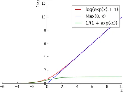
The vanishing gradient problem was not solved until 2010 by the introduction of the Rectified Linear units (ReLU) [9]. The activation function of ReLU units is defined as:

f(x) = ∞

X

i=1

(31)

2.4. DEEP LEARNING

The softmax function log(1 +ex_{) can be approximated by the max function} or hard-max function f(x) = max(0, x).

Figure 2.5 presents a graphically comparison between the ReL and the sig-moid function.

Figure 2.5: ReL and sigmoid functions comparison The main difference between both functions is that:

• The sigmoid function has range [0,1] while the ReL function has range [0,∞).

• The gradient of the sigmoid function vanishes as it is increased or de-creased x while the gradient of the ReL function doesn’t vanish as x is increased.

2.4.2 Gradient Descent Optimization Algorithms

There are three variants of the gradient descent algorithm, which differ in

(32)

2.4. DEEP LEARNING

1. Batch Gradient Descent. It computes the gradients for the loss function L(W,b) for the entire training set. It guarantees the convergence to the global minimum for convex error surfaces and to a local minimum for non-convex surfaces.

2. Stochastic Gradient Descent. It performs a parameter update for each training example xi _{and label} _yi_{. It is used for online learning as it} performs one update at a time. It enables to jump to new and potential better local minimum but complicates the convergence to the exact local minimum.

3. Mini-batch Gradient Descent[17]. It computes the gradients for the loss function L(W,b) only for a small batch of n training samples. Its faster than batch gradient descent and leads to a better convergence than stochastic gradient descent.

Next it is presented an outline of some algorithms used in deep learning to optimize the gradient descent algorithm.

1. Momentum [25]

The simplest gradient algorithm known as steepest descent 2.1.4, mod-ifies the weight at time step t according to:

W_i,jl =W_i,jl −α ∂ ∂Wl i,j L(W, b) bl_i =bl_i−α ∂ ∂bl i L(W, b)

However, it is known that learning such scheme can be very slow. To improve the speed of convergence of the gradient descent algorithm it is included the momentum term in the formula:

W_i,j,tl ₊₁ =W_i,j,tl −α ∂ ∂Wl

i,j

(33)

2.4. DEEP LEARNING

bl_i,t₊₁ =bl_i,t−α ∂ ∂bl

i

L(W, b) +γbl_i,t

where γ is the momentum term. In consequence, the modification of the weight vector at the step t depends on both the current gradient and the weight change of the step t−1.

2. Adagrad [5]

Adagrad is an algorithm for gradient-based optimization that adapts the learning rate to the parameters, performing smaller updates for frequent parameters and larger updates for infrequent parameters. Adagrad uses a different learning rate for every parameterWl

i,j,tat each time step t. In its update rule, it modifies the general learning rateαat each time step t for every parameterW_i,j,tl based on the past gradients that have been computed for W_i,j,tl .

W_i,j,tl ₊₁ =W_i,j,tl − α Gl t,ij+ ∗ ∂ ∂Wl i,j L(W, b) where Gl

t,ij ∈Rdxd is the diagonal matrix where each diagonal element ij is the sum of the squares of the gradients Wl

i,j,t+1 up to time stept24

and is smoothing term that avoids division by zero (≈1e−8). 3. Adam [13]

Adam is the acronym for Adaptive Moment Estimation. It is another method that computes adaptive learning rates for each parameter. It stores an exponentially decaying average of the past squared gradients that we will denotavt and similar to momentum, it keeps an exponen-tially decaying average of past gradients mt:

mt=β1mt−1+ (1−β1)∗gtvt=β2vt−1+ (1−β2)∗gt2

(34)

2.4. DEEP LEARNING

and the second moment or uncentered variance of the gradients, respec-tively. mt and vt are initialized as vectors of 0’s and in consequence, during initial time steps and when the decay rates are small they tend to be biased towards 0. To solve this problem, they computed the bias-corrected first and second moment estimates:

ˆ mt= mt 1−βt 1 ˆ vt= vt 1−βt 2

As a result, the Adam update rule is defined as:

Wt+1 =Wt− α √ ˆ vt+ ∗mˆt

(35)

Chapter 3 State of the Art

During the last decade, researchers and anti-virus vendors have begun em-ploying machine learning algorithms like the Association Rule, Support Vec-tor Machines, Random Forests, Naive Bayes and Neural Networks to address the problem of malicious software detection and classification. An overview of the methods can be found in [26], [7] and [6]. Following a few of these approaches used in literature are discussed.

1. Byte-sequence N-grams[33, 31]

The representation of a malware file as a sequence of hex values can be effectively described through n-gram analysis. A N-gram is a contigu-ous sequence of n hexadecimal values from a given malware file. Each element in the byte sequence can take one out of 257 different values, i.e. the 256 byte range plus the special ‘??’ symbol. Byte-sequence N-grams were first presented in [33], where they proposed a N-gram based algorithm for malware classification implemented in IBM’s an-tivirus scanner. The algorithm used 3-grams as features and a neural network as a classification model. Notice that the size of the features increase exponentially being 2562 for a bigram model and 2563 for a tri-gram model being the techniques for dimensionality reduction a must

(36)

2. Opcodes N-grams [11, 27, 2, 3, 30]

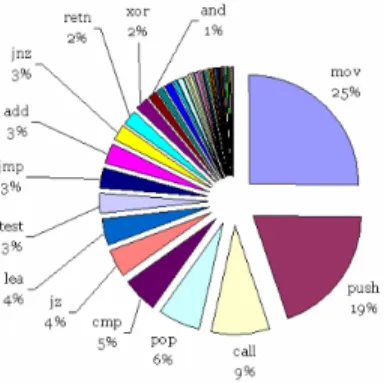
Similar to byte-sequence N-grams, n-gram models have been generated from opcodes extracted from assembly language code files. An opcode (abbreviated from operation code) is the portion of a machine language instruction that specifies the operation to be performed. In particular, [3] investigated the most frequent opcodes and the rare opcodes present in both goodware and malware. The following two charts show the 14 most frequent opcodes in goodware and in malware, respectively.

Figure 3.1: Most frequent 14 opcodes for goodware

Figure 3.2: Most frequent 14 opcodes for malware

3. Portable Executable [37, 28]

(37)

com-monly used in the Windows operating systems. PE format is a data format that encapsulates the necessary information for the Windows OS loader to manage the executable code. It includes information such as dynamic library references for linking and API import and export tables.

Features from Portable Executables (PE) are extracted by perform-ing static analysis usperform-ing structural information of PE and are useful to indicate whether or not the file has been manipulated or infected to perform malicious activity. In [37] they extracted the following fea-tures from PE: (1) File pointers which denote the position within the file as it is stored on disk; (2) Import sections which describe functions from which DLLs were used and the list of DLLs of the executable that are imported; (3) Exports section which describes the functions that are exported; (4) Structure of the PE header such as features like the code and file size, the creation time, etc. After the feature extrac-tion process they build an ensemble of support vector machines. The training set consisted of 9838 executables, from which 2320 were be-nign executables, 1936 backdoors, 1769 spyware, 1911 trojans and 1902 worms. They tested the performance of the classifier on two datasets: (1)Malfease and (2)VXheavens.

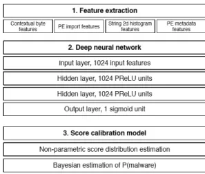
In [28], Invencea Labs build a Deep Neural Network to detect malware by using a set of features derived from the numerical fields extracted from the file binary’s PE packaging. The Deep NN consisted of three layers: the input layer of 1024 input features and two hidden layers of 1024 PReLU units each one. The output layer consisted of one sigmoid unit denoting whether the file is goodware or malware. In the following picture you can see an outline of the framework.

(38)

Figure 3.3: Outline of Invencea’s Malware Detection Framework

4. Entropy [29, 18]

Malware authors use obfuscation techniques to pass through signature-based detection systems of antivirus programs. For this reason, it is examined the statistical variation in malware samples to identify packed and encrypted samples. In [18] it was presented a tool to analyze the entropy of each PE section in order to determine which executable sections might be encrypted or packed. They found that the average entropy is 4.347, 5.099, 6.801, 7.175 for plain files, native executables, packed executables and encrypted executables, respectively.

5. API calls [4, 36]

API and function calls have been widely used to detect and classify malicious software. An experiment was conducted to determine the top maliciously used APIs. They retrieved the imports of all of the PE files and proceeded to count the number of times each sample uniquely imported an API. They found that there was a total of 120126 uniquely imported APIs.

(39)

API call sequences. They used a 3rd order Markov chain, i.e. 4-grams, to model the API calls. The malicious executables mainly consisted of backdoors, worms and Trojan horses collected from VXHeavens. Their detection system achieved an accuracy of 90%.

6. Use of registers

In [19], they proposed a method based on similarities of binaries behav-iors. They assumed that the behavior of each binary can be represented by the values of memory contents in its run-time. In other words, values stored in different registers while malicious software is running can be a distinguishing factor to set it apart from those of benign programs. Then, the register values for each API call are extracted before and after API is invoked. After that, they traced the changes of registers values and created a vector for each of the values of EAX, EBX, EDX, EDI, ESI and EBP registers. Finally, by comparing old and unseen malware vectors they achieved an accuracy of 98% in unseen samples. 7. Call Graphs

A call graph is a directed graph that represents the relationships be-tween subroutines in a computer program. In particular, each node represents a procedure/function and each edge (f,g) indicates that pro-cedure f call propro-cedure g. This kind of analysis have been used for malware classification with good results. In [15], they presented a framework which builds a function call graph from the information extracted from disassembled malware programs. For every node (i.e. function) in the graph, they extracted attributes including library APIs calls and how many I/O read operations have been been made by the function. Then, they computed the similarity between any two mal-ware instances.

(40)

8. Malware as an Image

In [21] a completely different approach to characterize and analyze ma-licious software was presented. They represented a malware executable as a binary string of zeros and ones. Then, the vector was reshaped into a matrix and the malware file could be viewed as a gray-scale image. They were based on the observation that for many malware families, the images belonging to the same family appear to be very similar in layout and texture.

Figure 3.4: Visualizing Malware as an Image

In addition, to compute texture features from malware images they used GIST[34, 23]. For classification, they used k-nearest neighbors with Euclidean distance and they obtained a classification rate of 0.9929 performing as state of the art results in the literature but at a signifi-cantly less computational cost.

(41)

Chapter 4 Microsoft Malware

Classification Challenge

The content of this chapter is structured as follows. First of all, it is presented the Microsoft Malware Classification Challenge and the platform where the competition was hosted. Secondly, it is described the winner’s solution of the challenge and the set of techniques they used to win the competition followed by an approach that achieved a logloss of 0.0064 and used features extracted from gray-scale images of malware. Lastly, it is presented the deep learning library used to implement the neural networks.

4.1 What’s Kaggle?

Kaggle is a platform where a large community of data scientist comprised from thousands of MsCs and PhDs from fields such as computer science, statistics and maths compete to solve valuable problems. These problems come from competitions that companies host in Kaggle or from competitions that are part of class homework or projects in academic institutions.

(42)

4.2. MICROSOFT MALWARE CLASSIFICATION CHALLENGE

4.2 Microsoft Malware Classification Challenge

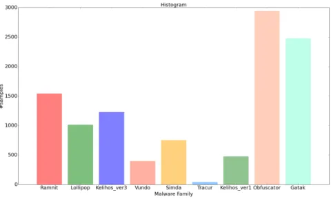
In 2015, Microsoft hosted a competition in Kaggle with the goal of classifying malware into their respective families based on the their content and charac-teristics. For this challenge, Microsoft provided a dataset of 21741 samples, with 10868 for training and the other 10873 for testing, being a dataset of almost half a terabyte uncompressed. Microsoft provided a set of malware samples representing 9 different malware families. Each malware sample had an Id, a 20 character hash value uniquely identifying the sample and a class, an integer representing one of the 9 malware family names to which the mal-ware belong: (1) Ramnit, (2) Lollipop, (3) Kelihos_ver3, (4) Vundo, (5) Simda, (6) Tracur, (7) Kelihos_ver1, (8) Obfuscator.ACY, (9) Gatak. The distribution of classes present in the training data is not uniform and the number of instances of some families significantly outnumbers the instances of other families.

Figure 4.1: Malware Classification Challenge: dataset

(43)

hexadec-4.2. MICROSOFT MALWARE CLASSIFICATION CHALLENGE

imal representation of the file’s binary content and a file containing metadata information extracted from the binary content, such as function calls, strings, sequence of instructions and registers used, etc, that was generated using the IDA disassembler tool.

4.2.1 Bytes file

The bytes file is the raw hexadecimal representation of the malware’s binary content. A snapshot of one of these bytes files is shown below.

Figure 4.2: Snapshot of one bytes file Each record of the hexadecimal files is composed by:

• Byte Count. Two hex digits indicating the number of hex digits pairs in the data field.

• Address. Four hex digits representing the 16-bit beginning memory address offset of the data.

• Record Type. Two hex digits, 00 to 05, defining the meaning of the data field.

(44)

• Checksum. Two hex digits, a computed value that can be used to verify the record has no errors.

4.2.2 ASM file

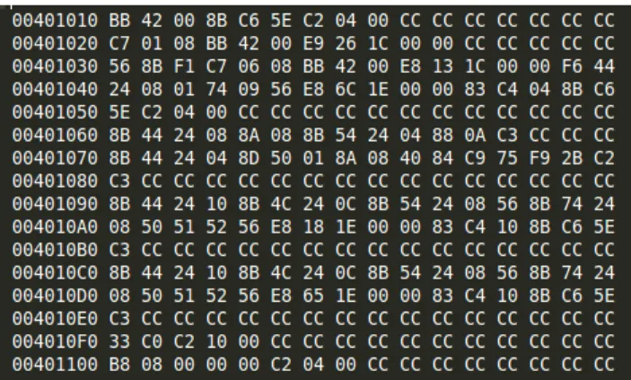
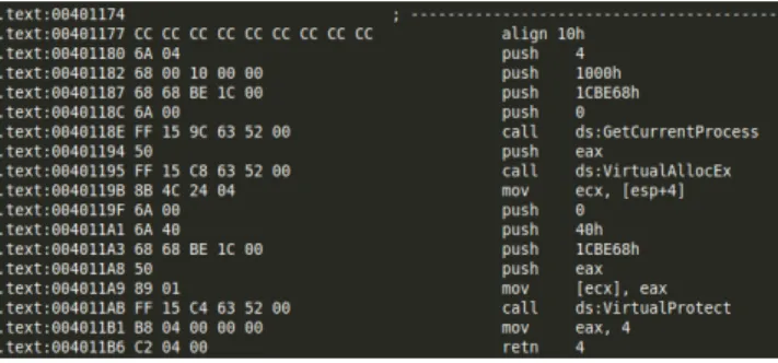
The asm file, generated by the disassembler tool, is a log containing vari-ous metadata such as rudimentary function calls, memory allocation, and variable manipulation. A snapshot of one of these files is shown below.

Figure 4.3: Snapshot of one assembly code file An assembly program is often divided into three sections:

1. The data section. It is used to declare initialized data or constants and do not change at runtime.

2. The bss section. It is used for declaring variables. Contains uninitial-ized data.

3. The text section. It keeps the actual code of the program.

Apart from the previous sections, an assembly program can contain other sections such as:

• The rsrc section. It contains all the resources of the program.

• The rdata section. It holds the debug directory which stores the type, size and location of various types of debug information stored in the file.

(45)

• The idata section. It contains information about functions and data that the program imports from DLLs.

• The edata section. It contains the list of the funcions and data that the PE file exports for other programs.

• The reloc section. It holds a table of base relocations. A base relocation is an adjustment to an instruction or initialized variable value that’s needed if the loader couldn’t load the file where the linker assumed it would.

Additionally, some other sections can appear as a result of applying a poly-morphic or metapoly-morphic techniques to hide the actual code.

The assembly language consists of three types of statements:

1. Instructions or assembly language statements. Are used to tell the processor what to do. Instructions are entered one instruction per line. Each instruction has the following format:

[ l a b e l ] mnemonic [ o p e r a n d s ] [ ; comment ]

where the fields in brackets are optional. A basic instruction has two parts: (1) the name of the instruction or the mnemonic to be executed (also known as opcodes); (2) the operands or the parameters of the command.

INC COUNT ; I n c r e m e n t t h e memory v a r i a b l e COUNT MOV TOTAL, 48 ; T r a n s f e r t h e v a l u e 48 i n t h e

; memory v a r i a b l e TOTAL

Next you will find the top 10 most used x86 instructions in the training dataset.

(46)

Figure 4.4: Top 10 opcodes in the training dataset

In addition, the average of instructions per each malware family is the following.

(47)

One particularity of the training dataset is that there are some mal-ware samples that due to code obfuscation techniques do not have any instruction. #samples Ramnit 0 Lollipop 2 Kelihos_ver3 4 Vundo 22 Simda 0 Tracur 0 Kelihos_ver1 6 Obfuscator.ACY 9 Gatak 0

Table 4.1: Number of samples per class with 0 instructions

2. Assembler directives or pseudo-ops. Are commands part of the assem-bler syntax but are not related to the x86 processor instruction set. All assembly directives start with a period (.).

. dat a . b s s

The .data and .bss directives change the current section to .data or .bss, respectively.

3. Macros. Are basically a text substitution mechanism. A macro is a se-quence of instructions, assigned by a name and could be used anywhere in the program. The syntax for a macro definition is:

%macro macro_name number_of_params <macro body>

(48)

4.3. WINNER’S SOLUTION

4.3 Winner’s solution

The competition was won by a team of three people, Jiwei Liu and Xueer Chen from the University of Pittsburgh and Xiaozhou Wang from Redman Technologies Inc. Their solution relied mainly in the extraction of the three following features from malware.

1. Opcode 2,3 and 4-grams.

• They counted the frequent 1-gram opcodes by selecting only the opcodes that appear more than 200 times in at least one asm file and they ended up with 165 features.

• All possible 2-gram counts were included (27225 features)

• The 3-gram and 4-gram counts which were greater than 100 in at least one asm file were also included (21285 and 22384 features, respectively)

2. Segment line count. They counted the number of lines per section in the asm file and they also counted the number of different sections in all malware samples which curiously was 448 a number much greater than 9, the number of sections in which an asm is usually divided. That’s because of the application of metamorphic and polymorphic techniques. 3. Asm file pixel intensity features. Instead of representing the bytes file as pixels they read the asm file as a binary file. They found that the first 800 pixel intensities were very useful features.

Then, they used XGBoost(a machine learning library focused on gradient boosted trees) and cross-validation to find the subset of features that best classified the malware in classes and they finally obtained the lowest public and private logloss of 0.003082695 and 0.002833228, respectively. In the next figure you can find the confusion matrix of the training data.

(49)

4.4. NOVEL FEATURE EXTRACTION, SELECTION AND FUSION FOR EFFECTIVE MALWARE FAMILY CLASSIFICATION

Ramnit Lollipop Kelihos_ver3 Vundo Simda Tracur Kelihos_ver1 Obfuscator.ACY Gatak

Ramnit 1541 0 0 0 0 0 0 0 0 Lollipop 1 2476 0 0 0 1 0 0 0 Kelihos_ver3 0 0 2942 0 0 0 0 0 0 Vundo 0 0 0 475 0 0 0 0 0 Simda 2 0 0 0 39 1 0 0 0 Tracur 1 0 0 0 0 750 0 0 0 Kelihos_ver1 0 0 0 0 0 0 398 0 0 Obfuscator.ACY 0 0 1 0 0 0 0 1225 2 Gatak 0 1 0 0 0 0 0 5 1007

Table 4.2: Winner’s solution: confusion matrix

where they classified correctly 10854 of 10868 samples (0,9987%).

4.4 Novel Feature Extraction, Selection and

Fusion for Effective Malware Family

Clas-sification

In [1] they presented an approach that extracts and combines different char-acteristics from malware and their fusion according to a perclass weighting paradigm. Their method achieved an accuracy of 0.998% on the Microsoft Malware Challenge dataset but what is more interestingly about their ap-proach is that they also extracted feature patterns from images of malware. Next you will find the different extracted set of features.

1. N-Gram (1G and 2G):

1-Gram and 2-Gram features from the hexadecimal representation of bi-nary files described with a 256-dimensional vector and 2562_-dimensional

vector for the 1-Gram and 2-Gram models, respectively. 2. Metadata (MD1 and MD2):

They extracted the size of the file and the address of the first byte sequence.

(50)

3. Entropy (ENT):

Entropy can be defined as a measure of the amount of the disorder and it is used to detect the presence of obfuscation in malware files and for this reason they computed the entropy of all the bytes in a malware file.

4. Image patterns (IMG1 and IMG2):

They extracted the Haralick features and the Local Binary Patterns features from each malware sample represented as a gray-scale image. 5. String length (STR):

They extracted possible ASCII strings and its length from each PE using its hex dump.

6. Symbol frequencies (SYM):

The frequencies of the symbols -, +, *, ], [, ?, @ are extracted from the disassembled files because are typical of code designed to evade detection by resorting to indirect calls or dynamic library loading. 7. Operation code (OPC):

They counted the number of times a subset of 98 operation codes ap-peared in each disassembled file. These subset was selected based either on their commonness or on their frequent use in malicious applications. 8. Register (REG):

They computed the frequency of use of the registers in x86 architecture. 9. Application Programming Interface (API):

They measured the frequency of use of the top 794 frequent APIs used in malware binaries based on the analysis performed in https://www.

bnxnet.com/top-maliciously-used-apis/.

10. Section (SEC):

(51)

disassem-4.4. NOVEL FEATURE EXTRACTION, SELECTION AND FUSION FOR EFFECTIVE MALWARE FAMILY CLASSIFICATION

bly files such as the total number of lines in .bss, .txt, .data, etc sections or the proportion of lines in each section compared to the whole file. 11. Data Define (DP):

They computed the frequency of db, dw and dd instruction because there are malware samples that do not contain any API call and only contain few operation codes, because of packing.

12. Miscellaneous (MISC):

This features are composed by the frequency of 95 keywords manually chosen from the disassembled code.

Following you will find a table containing the list of feature categories and their evaluation with XGBoost.

Feature Category #Features Accuracy Logloss

ENT 203 0.9987 0.0155 1G 256 0.9948 0.0307 STR 116 0.9877 0.0589 IMG1 52 0.9718 0.1098 IMG2 108 0.9736 0.1230 MD1 2 0.8547 0.4043 MISC 95 0.9984 0.0095 OPC 93 0.9973 0.0146 SEC 25 0.9948 0.0217 REG 26 0.9932 0.0352 DP 24 0.9905 0.0391 API 796 0.9905 0.0400 SYM 8 0.9815 0.0947 MD2 2 0.7655 0.6290

Table 4.3: List of feature categories and their evaluation in XGBoost After the feature extraction process, they combined the features using a version of the forward stepwise selection algorithm. The original version of

(52)

increases the feature set by adding one feature at each iteration. Instead of considering one feature at a time, they added all the subset of features belonging to a feature category at a time, until when adding more features didn’t increase the value of logloss. By combining the feature categories as described earlier, they achieved a test logloss of 0.0063 positioning its solution among the top 10 in the competition.

(53)

4.5. DEEP LEARNING FRAMEWORKS

4.5 Deep Learning Frameworks

Deep Learning is a hot field in Artificial Intelligence and Machine Learning, and thus, there are various deep learning libraries available open-source. The most popular are:

1. Caffe.

It is a python deep learning framework developed by the Berkeley Vi-sion and Learning Center. It allows you to define if train using the CPU or the GPU easily. Caffe benefits from having a huge repository with pre-trained neural network models suited for many problems. It has a great implementation for convolutional networks but it has no implementation for recurrent networks.

2. Theano.

It is a python deep learning library which make use of symbolic graph for programming the networks. It also allows you to visualize the com-putation graphs with d3viz.

3. TensorFlow.

It is written with a Python API over a C/C++ engine that makes it run fast. It is more than a deep learning framework, and it has tools to support reinforcement learning and other algorithms. In addition, Ten-sorFlow can also be deployed in phones thanks that it can be compiled in ARM architectures.

4. Deeplearning4j.

It is a deep learning framework developed in Java. It aims to be the scikit-learn library in the deep learning space.

5. Torch.

(54)

4.5. DEEP LEARNING FRAMEWORKS

Google and Facebook. However, it is not as well-documented as other deep learning frameworks.

TensorFlow has been chosen mainly because it has a Python API, there’s a lot of documentation available and it has a large community that it con-tinuously develops the library. In addition, it is very easy to setup and to learn and recently, they released TensorBoard, a tool to visualize TensorFlow graphs and to plot some metrics such as the accuracy or the loss at each train-ing iteration. Moreover, it provides support for distributed computtrain-ing since version 0.8 (currently 0.11).

(55)

Chapter 5 Learning Feature Extractors

from Malware Images

The problem of malware detection and classification is a very complex task and there’s no perfect approach to tackle it. For this reason AV vendors rely in hybrid approaches that make use of traditional signature-based, heuristic-based and machine learning methods as well as human analysis.

This chapter presents a novel approach for malware classification based on the work performed by Nataraj et al. [21] which introduced the idea of representing malicious software as gray-scale images. Then, they extracted different features using GIST and they used the k-nearest neighbor algorithm for classification. Our approach differ in the point that we use Convolutional Neural Networks for learning discriminative patterns from the malware im-ages.

The next sections explain how malware can be visualized as images followed by the architectures of the different CNNs tested and its specifications as well as the results obtained in the Kaggle’s competition.

(56)

5.1. VISUALIZING MALWARE AS GRAY-SCALE IMAGES

5.1 Visualizing malware as gray-scale images

This thesis is highly motivated by the work in [21] which is based on the observation that images of different malware samples from the same family appear to be similar while images of malware samples belonging to a differ-ent family are distinct. Moreover, if old malware is re-used to create new malware binaries the resulting ones would be very similar visually.

In their work, they computed image based features to characterize malware. For that purpose, to compute texture features they used GIST [24]. The resulting feature vectors were used to train a K-nearest neighbor classifier with Euclidean distance. As introduced in [21], a given malware binary file can be read as a vector of 8 bit unsigned integers and organized into a 2D array. Then, this array can be visualized as a gray scale image in the range [0,255].

Figure 5.1: Visualizing Malware as a Gray-Scale Image

The main benefit of visualizing malware as an image is that the different sections of a binary can be easily differentiated. In addition, as malware au-thors only change a small part of the code to produce new variants, images are useful to detect small changes while retain the global structure. In con-sequence, malware variants belonging to the same family appear to be very similar as images while also being distinct from images of other families.

(57)

5.1.1 Malware families

Following are presented some malware files of each malware variant in the dataset. One particularity of the dataset is that the samples do not contain the PE header because it was removed to ensure sterility.

1. Ramnit. This type of malware is known to steal your sensitive infor-mation such as user names and passwords and it also can give access to an illegitimate user to your computer.

Figure 5.2: Rammit samples

2. Lollipop. This malware shows ads in your browser and redirects your search engine results. In addition, it tracks what you are doing on your computer. This type of malware usually is downloaded from the pro-gram’s website or by some third-party software installation programs.

Figure 5.3: Lollipop samples

3. Kelihos_ver3. Third version of the Kelihos botnet. Kelihos is mainly involved in spamming and theft of bitcoins. This trojan can give ac-cess and control of your computer to an illegitimate user and can also communicate with other computers about sending spam emails, run malicious programs and steal sensitive information.

(58)

Figure 5.4: Kelihos_ver3 samples

4. Vundo. This trojan is known to cause popups and advertising for rogue antispyware programs. In addition, sometimes is used to perform denial of service attacks and also to deliver malware to other computers.

Figure 5.5: Vundo samples

5. Simda. It is a family of backdoors that try to steal sensitive information such as usernames, passwords and certificates via its keylogging and HTML injection routines. It also can give a hacker access to your computer.

Figure 5.6: Simda samples

6. Tracur. This trojan hijacks results from different search engines such as google, youtube, yahoo, etc, and redirects to a different web page. It also give a hacker access to your computer and can be used to download other types of malware.

(59)

Figure 5.7: Tracur samples

7. Kelihos_ver1. First version of the Kelihos botnet. It was first discov-ered at the end of 2010 having infected 45.000 machines and sending about 4 billions spam messages per day.

Figure 5.8: Kelihos_ver1 samples

8. Obfuscator.ACY. This class comprises all malware that has been ob-fuscated to hide their purposes and to not be detected. The malware that lies underneath this obfuscation can have almost any purpose.

Figure 5.9: Obfuscator.DCY samples

9. Gatak. It is a trojan that gathers information about your pc and sends it to a hacker. It also downloads other malware files in your computer. This trojan is usually downloaded when downloading a key generator or a software crack.

(60)

(61)

5.2. CNN ARCHITECTURES

5.2 CNN Architectures

In this thesis, we have proposed a novel approach to classify samples of malicious software from their representation as gray-scale images. In the work of [21] they used a traditional recognition approach to classify gray-scale images of malware. First of all they extracted texture features from the malware gray-scale images and then, they trained a K-NN classifier.

Figure 5.11: Shallow Approach

The main problem of their approach is that it doesn’t scales well with lots of data. Accordingly, two ways of improvement are (1) keep building more features like SIFT, HoG, etc and (2) using another classifier like Random Forests or SVM. Instead, our approach makes use of Convolutional Neural Networks to learn a feature hierarchy all the way from pixels to the layers of the classifier.

This section presents the different architectures of the network and its spec-ifications. The details of the architectures are defined in figures 5.12, 5.13 and 5.14.

All architectures have in common the input and the output layers. On one hand, the input layer consists of N neurons, being N the size of the training images. The image and the height of the images varies depending on the file

(62)

size and thus, before feeding the images as input all images had been down-sampled to 32 by 32 pixels. In consequence, N is equals to 32∗32 = 1024. On the other hand, all architectures have an output layer of 9 neurons because the architectures are designed to handle a 9-class classification problem. In addition, after each densely-connected layer it was applied dropout to reduce overffiting.

To determine the parameters for each architecture it was performed a grid search. Specifically, the grid search was used to determine the optimum learn-ing rate, the size of the kernels of each convolutional layer and the number of filters applied and also the number of neurons in each densely-connected layer. Finally, to reduce the search space some parameters were fixed such as the mini-batch size to 256, the region of the max-pooling layer to 2x2 with stride equals to 2 and the learning rate to 0.001

(63)

5.2.1 CNN A: 1C 1D

The architecture consists of:

1. Input layer of NxN pixels (N=32).

2. Convolutional layer (64 filter maps of size 11x11). 3. Max-pooling layer.

4. Densely-connected layer (4096 neurons) 5. Output layer. 9 neurons.

The input layer consists of 32x32 neurons and is followed by a convolutional layer composed by 64 filters of size 11x11. The output of the convolutional layer is (32−11 + 1)∗(32−11 + 1) = 22∗22 = 484 for each feature map. As a result, the total output of the convolutional layer is 22∗22∗64 = 30976. After that, the pooling layer takes the output of each feature map from the con-volutional layer and outputs the maximum activation of all 2x2 regions. In consequence, the output of the pooling layer is reduced to 11∗11∗64 = 7744. The pooling layer is then followed by a fully-connected layer with 4096 neu-rons and every neuron of this layer is also connected to each one of the neurons in the output layer.

The number of learnable parameters P of this network is:

P = 1024∗(11∗11∗64)+64+(11∗11∗64)∗4096+4096+4096∗9+9 = 39690313 where (11∗11∗64) + 64 are the shared weights for every feature map and 64 is the total number of shared bias.

(64)

Figure 5.12: Overview architecture A: 1C 1D

5.2.2 CNN B: 2C 1D

The architecture consists of:

1. Input layer of NxN pixels (N=32).

6. Densely-connected layer (512 neurons). 7. Output layer. 9 neurons.

As in the previous architecture, the input layer consists of 32x32 neurons and is followed by a convolutional layer composed by 64 filters of size 3x3. The

Convolutional neural networks for malware classification