automatic group learning
.
White Rose Research Online URL for this paper:
http://eprints.whiterose.ac.uk/126298/
Version: Accepted Version
Proceedings Paper:
Partov, B., Leith, D.J. and Checco, A. orcid.org/0000-0002-0981-3409 (2017)
Recommending access points to individual mobile users via automatic group learning. In:
IEEE International Conference on Communications. 2017 IEEE International Conference
on Communications (ICC), 21-25 May 2017, Paris, France. IEEE . ISBN 9781467389990
https://doi.org/10.1109/ICC.2017.7997424
© 2017 IEEE. Personal use of this material is permitted. Permission from IEEE must be
obtained for all other users, including reprinting/ republishing this material for advertising or
promotional purposes, creating new collective works for resale or redistribution to servers
or lists, or reuse of any copyrighted components of this work in other works. Reproduced
in accordance with the publisher's self-archiving policy.
[email protected] https://eprints.whiterose.ac.uk/
Reuse
Unless indicated otherwise, fulltext items are protected by copyright with all rights reserved. The copyright exception in section 29 of the Copyright, Designs and Patents Act 1988 allows the making of a single copy solely for the purpose of non-commercial research or private study within the limits of fair dealing. The publisher or other rights-holder may allow further reproduction and re-use of this version - refer to the White Rose Research Online record for this item. Where records identify the publisher as the copyright holder, users can verify any specific terms of use on the publisher’s website.
Takedown
If you consider content in White Rose Research Online to be in breach of UK law, please notify us by
Recommending Access Points to Individual Mobile
Users via Automatic Group Learning
Bahar Partov
1,2, Douglas J. Leith
1, and Alessandro Checco
31
Trinity College Dublin, Ireland,
2SENSEable City Lab, Massachusetts Institute of Technology, USA
3University of Sheffield, U.K.
Abstract: We consider user to cell association in a het-erogeneous network with a mix of LTE/3G and WiFi cells. Individual user preferences are often neglected when a user to cell association decision is made. In this paper we propose use of a recommender system to inform the mapping of users to cells. We demonstrate the effectiveness of the proposed grouped-based user to cell associations for a set of syntheti-cally generated user/cell ratings.
I. INTRODUCTION
In this paper we study the use of collaborative filtering based recommender systems to assist users with wireless access point selection. In metropolitan areas there is widespread avail-ability of both cellular and WiFi services. LTE/3G coverage is ubiquitous in urban areas. Many enterprises, schools, and cities provide WiFi services to individuals. Hotspot directories report large numbers of WiFi access points in urban areas, e.g. jiwire in the US reports 400 to 1000 commercial WiFi networks in each of the top ten U.S. metropolitan areas [1] and the Fon service has aggregated more than 3 million access points in the UK alone [2]. This is in addition to home-based WiFi services. Currently almost all mobile devices possess both cellular and WiFi interfaces, and smartphone users can, and do, switch among different WiFi access points and their cellular connection. Users therefore often have a great deal of choice but, currently, little information on which to base this decision other than the signal level bars displayed to them by their handset. Note that from now on we will use access point to interchangeably mean a WiFi access point or a cellular connection since our recommendation approach is agnostic to the wireless technology used. Unfortunately, signal strength by itself is often not a good indicator of the usefulness of an access point to a particular user: access points might block certain applications [3], may have different terms and conditions regarding user privacy, cost of the service etc and in other ways may have poorer performance than that proclaimed by the signal strength [4]. It is this observation which motivates the provision of recommendations to a user as to which of the access points available in a location are likely to be most satisfactory for that particular user.
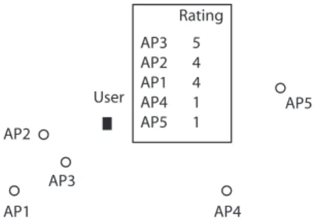
The setup we consider is illustrated schematically in Fig 1.
We have a set of nusers and m access points. After user u
makes use of an access point v they rate the utility provided
to them – this is a matter of personal preference that reflects
Work supported by SFI grant 11/PI/1177 and 13/RC/2077.
AP1 AP2 AP3 AP4 AP5 User AP3 5 AP2 4 AP1 4 AP4 1 AP5 1 Rating
Fig. 1: Illustrating the setup considered. A user is in an area with multiple access points (WiFi access points and LTE/3G cellular connections). In the past the user has rated a subset of these access points, as have other users. These ratings reflect user satisfaction and take account of aspects such as cost, applications blocked/allowed, congestion as well as signal strength. The aim is to use this data to collaboratively recommend to a user the access points which they are most likely to prefer.
the dollar price paid, ease of use, QoS, applications supported
and so on. Gathering these ratings together gives an n×m
ratings matrixR, where elementRuvis the rating by useruof
access pointv. This matrix is typically sparse, since each user
individually may rate only a small number of access points.
Our aim is to estimate the missing entries inR, i.e. to provide
predictions of the ratings a user would make for access points which are currently unrated. Those access points which are predicted to have a high rating are then recommended to a
user. In addition to the sparseness of rating matrix R, which
is common in recommender systems, challenges include the heterogeneity of the user population and the sensitivity of ratings (and so recommendations) to user location. It is these challenges which we seek to address in this paper.
Our main contributions are as follows. We propose a novel matrix factorisation based recommender approach for use with wireless access point data. This approach uses a mixture model to capture sensitivity of access point ratings to user location and clustering of users into a number of groups to capture user heterogeneity while still allowing accurate predictions when the ratings data is sparse. We evaluate the performance of this approach for a range of network conditions, including a realistic model of a downtown university campus.
II. RELATEDWORK
The task of recommending cell selection based on learning of user preferences has received very little attention in the literature to date. Of course there exists an extensive body of
research that highlight the benefits of offloading user traffic to the WiFi or unlicensed LTE networks [5] - [6]. However, the task of network selection is almnost always viewed as a network-wide utility optimisation problem whereby the network provider seeks to maximise data rates and/or min-imise delays. This work rarely takes much account of the requirements and preferences of the individual users. Today different WiFi APs and cellular providers offer a variety of services and a user can manually switch between different APs in order to identify its preferred AP. Users are typically only informed of the available access points and their associated signal quality. A notable exception is [7] in which a more sophisticated approach called WiFi-Reports is proposed. This is a collaborative service that provides WiFi clients with historical information about AP performance and application support i.e. beyond just signal strength.
III. PRELIMINARIES
Matrix factorization approaches are a popular and successful
way of making recommendations. The ratings matrix R ∈
Rn×mis modelled as the productUTV
of matrixU∈Rd×n
and matrixV ∈Rd×m. The idea is that the entries in column
Vv of matrixV capture the characteristics of resourcev as a
point in a latent d-dimensional feature space and the entries
of columnUuthe weights that useruattaches to these, so that
the rating of resourceuby useruis the inner productUuTVv.
Importantly, dis much smaller than either n orm. It is this
which allows predictions to be made even when the matrixR
is sparse.
To estimate U andV a common approach is to adopt the
following statistical model. The rating supplied by user ufor
resource v is a Gaussian random variable XRuv ∈ R with
mean UTuVv and variance σ2. That is,
P rob(XRuv =Ruv|U˜,V)∼e
−φuv(Ruv)/σ2
whereφuv(Ruv) := (Ruv−UuTVv)2. Let O ⊂ {1,· · ·, n} ×
{1,· · ·, m} denote the set of user-resource rating pairs that
are contributed by the users and ZO ={XRuv,(u, v)∈ O},
RO ={Ruv,(u, v) ∈ O}. The conditional distribution over
these observed ratings is,
P rob(ZO =RO|U,V) ∼
Y
(u,v)∈O
e−φuv(Ruv)/σ2
Assuming Gaussian priors forU andV with zero mean and
varianceσ2
U andσ2V˜, respectively, the log-posterior is then
− 1 σ2 X (u,v)∈O φuv(Ruv)− 1 σ2 U trUTU− 1 σ2 V trVTV +C (1)
where C is a normalising constant. We now estimate U
and V as the matrices which maximise this log-posterior.
Observe that since d is small this estimation can be carried
out successfully even when the set of observationsOis small
(i.e. the observed elements of matrix Rare sparse).
It is well known that users can often be grouped together by their preferences. For example, users in the same group may use similar mobile applications, have similar price sensitivity and so on. Following [8] this can be captured by further
factorising matrixUasU P˜ whereU˜ ∈Rd×pandP ∈Rp×n.
ColumnU˜g captures the preferences of theg’th group of users
(referred to as anymin [8]) andPuthe mapping from useru
to these groups. In [8] the elements ofP are{0,1}valued and
P is column stochastic (the columns sum to one) so that each
user is a member of a single group. By learningP as well asU˜
andV based on the observed data we can carry out automatic
clustering of users into groups in parallel with factorising the ratring matrix. With this change the log-posterior is now
− 1 σ2 X (u,v)∈O ˜ φuv(Ruv)− 1 σ2 ˜ U trU˜TU˜− 1 σ2 V trVTV +C (2)
with φ˜uv(Ruv) := (Ruv −(PU˜)TuVv)2. To maximise the
log posterior (2), we can apply an iterative algorithm which alternates between the following two steps:
1) Using the current estimates for the matrix of average
nym-item ratings R˜ and the numberΛ(v) of users in
each nym who rate item v, estimateU˜,V.
2) Given the current estimates for U˜, V each user u
updates their columnPu inP by solving
minPu∈I
P
v∈V(u)(Ruv − PTuU˜ T
Vv)2 where I =
{ei, i= 1, p},ei the vector for which elementiequals
1 and all other elements equal to0.
IV. RECOMMENDINGWIRELESSACCESSPOINTS
Our problem differs in a number of significant ways from the standard matrix factorisation setup outlined above. Perhaps the most important difference is that we expect the rating assigned by a user to an access point to depend on the user’s location. Namely, when close to an access point we expect that the rating may be higher than when further away. We do not, therefore, have a single rating by a user for an access point
and cannot construct a single rating matrix R of user-item
ratings.
A. Location-based Mixture Model
To accommodate this location dependence we propose the following mixture model approach. We begin by dividing
the geographical area A of interest into a set of (possibly
overlapping) smaller patchesAi⊂A,i= 1,2, . . . , qsuch that
∪qi=1Ai =A. These patches might, for example, be selected
to be centered on regions where the WiFi access points are most dense or based on local geographical knowledge. The
Ruv= q X i=1 d(u, i) Pq j=1d(u, j) Ri,uv (3)
whereRi∈Rn×mis a rating matrix associated with patchAi
(ratings made when users are located in patchi), andd(u, i)is
the distance between the current position of useruand patchi.
We will return to the choice of an appropriate distance metric
shortly. Decomposing Ri as UTVi and assuming Gaussian
priors on U, Vi and Gaussian noise on the ratings the
log-posterior is − 1 σ2 X (u,v)∈O ψuv(Ruv)− 1 σ2 ˜ U q X i=1 trUTU − 1 σ2 V q X i=1 trVT iVi+C (4)
withψuv(Ruv) := (Ruv−Pqi=1
d(u,i)
Pq j=1d(u,j)
UTu(Vi)v)2.
To allow automatic clustering of users into groups (which we refer to as automated group learning) we further factorise
U asU P˜ whereU˜ ∈Rd×pandP ∈Rp×n. With this change
the log-posterior becomes
− 1 σ2 X (u,v)∈O ˜ ψuv(Ruv)− 1 σ2 ˜ U q X i=1 trU˜TU˜ − 1 σ2 V q X i=1 trVT iVi+C (5) with ˜ ψuv(Ruv) := (Ruv−(U P˜ )Tu q X i=1 d(u, i) Pq j=1d(u, j) (Vi)v)2 (6)
Note that we use the same matrix P mapping from users to
groups for all patchesAisince we assume user preferences do
not change significantly with location. User preferences may, of course, vary with their role which in turn may vary with location, e.g. when at home and when at the workplace, but we can capture this within our model by treating a change in role as effectively the introduction of a new user.
B. Learning Algorithm
We assume1 that the set of patches A
i, i = 1, . . . , q is
given and also the distance metricd(u, i). This allows existing
matrix factorisation approaches to be applied in a relatively straightforward manner. Namely, to maximise the log posterior (5), we can apply an iterative algorithm which alternates between the following two steps:
1) Using the current estimates for the matrix of group-item
ratingsR˜i:= ˜UTVi in patchAi and the numberΛ(v)
of users in each group who rate itemv, estimate each
of U˜, Vi, i = 1, . . . , q in turn. That is, we first hold Vi, i = 1, . . . , q fixed and estimate U˜ then hold U˜
fixed and estimate Vi in turn for i = 1, . . . , q. Each
of these optimisations is convex and, indeed, is just a least squares problem and so its solution is known in closed-form.
2) Given the current estimates for U˜, Vi each user u
updates their columnPu inP by solving
min Pu∈I X v∈V(u) (Ruv−P T uU˜ T q X i=1 d(u, i) Pq j=1d(u, j) (Vi)v)2 (7) where2 I = {e
i, i = 1, p}, ei the vector for which
elementiequals1and all other elements equal to0. This
optimisation is non-convex but can be trivially solved 1Local geographical information is often available that makes defining the
patchesAirelatively straightforward e.g. using knowledge of buildings with
many access points where users tend to congregate. Alternatively, clustering approaches such as k-nearest neighbours might be used to induce patches based on measurements but we leave this as future work.
2Note that it is straightforward to extend consideration to vectorsP
uwhich
are not restricted to be(0,1)valued but this comes at the cost of increased computational complexity and potentially also reduced privacy since when Puis (0,1) valued step 2 can be efficiently carried out locally within a
users mobile handset. Although we do not consider privacy further here due to lack of space, it is increasingly recognised as being an important issue in recommender systems e.g. see [8] and references therein.
by simply calculating the objective for each element in
(small) set I and selecting the lowest valued.
C. Convergence
We omit the proof for sake of brevity but it can be readily verified that each step of the learning algorithm in Section IV-B is a descent update. Hence, the algorithm is guaranteed to converge to a stationary point of the log-posterior. Since the log-posterior is non-convex (even though it is convex in
P,U˜,Vi,i= 1, . . . , qindividually it is not jointly convex in
these matrices) we have no guarantee that the stationary point to which the algorithm converges is not a local minimum or even a saddle point. However, by starting from a number of different initial conditions we can gain some confidence in its convergence to a reasonable point and, as we will see in the next section, experimental studies indicate that convergence is typically both fast and to a reasonable minimum.
V. PERFORMANCEEVALUATION
We evaluate the performance of the proposed access point recommender system with automatic group learning using synthetic datasets, i.e. where we know the ground truth. A. User Rating Model
For evaluation purposes we model the ratingRu,aof access
pointaby userulocated in patchAi as
Ri,ua =si,ua− Cu (8)
wheresi,ua is the data rate of useruwhen using access point
a from patch Ai andCu denotes the cost of user u(e.g. the
cost charged for data access).
Having the user rating depend on the achieved rate si,ua
is natural. For our evaluation we assume that users belong to
one of two groups, namely have eitherCu:= 0 orCu:= 25.
This allows us to capture, albeit in a crude way, users with differing price sensitivities. Users are assigned uniformly at random to one of these two groups. This simple model neglects the impact of e.g. blocking of certain applications by access points, but can be readily extended to include such effects. B. Small Geographic Area
We begin by considering a small geographic area
corre-sponding to a single patch Ai within which user ratings
are captured by rating matrix Ri. We will consider a more
accurate path loss model shortly, but initially we let the rate
sua of user u when using access point a be drawn from a
Gaussian distribution with mean µs and standard deviation
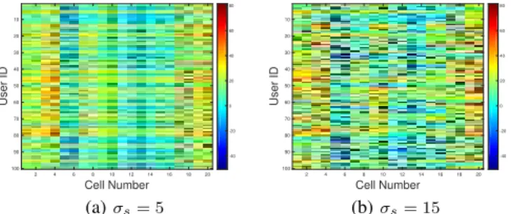
σs. Fig 2 illustrates the corresponding user ratings (9) for two
example realisations. In the left-hand plot the variance σs of
the ratessua is relatively small and the presence of two groups
of users is evident. In the right-hand plot the variance in the rates is higher with the result that the user ratings are also more variable.
Unless otherwise stated we use the network settings and recommender system parameters summarised in Table I. We measure the performance of the recommender system by
2 4 6 8 10 12 14 16 18 20 Cell Number 10 20 30 40 50 60 70 80 90 100 User ID -40 -20 0 20 40 60 80 (a)σs= 5 2 4 6 8 10 12 14 16 18 20 Cell Number 10 20 30 40 50 60 70 80 90 100 User ID -40 -20 0 20 40 60 80 (b)σs= 15
Fig. 2: Illustrating the full user ratings matrix whenµs= 50Mbps.
Parameter Value
Network
Number of cells (m) 20
Mean users’ throughput (µs) 50
Standard deviation of users’ throughput (σs) 10
Learning Algorithm
Number of groups (p) 2
Dimension of the feature space (d) 2
Number of runs 10
TABLE I: Network and recommender system parameters.
holding back a subset consisting of 20% of the ratings selected uniformly at radnom without replacement and then calculating the root mean square (RMSE) between the predicted ratings
Pq i=1
d(u,i)
Pq j=1d(u,j)
UTViand true user ratingsRin this subset.
Results shown are the mean and standard deviations over at least 10 random realizations.
1) Prediction error vs. number of groups used and sparsity of ratings: Figure 3(a) illustrates the impact of the number of groups used on the automatic group learning algorithm (i.e.
when grouping matrixP is estimated and the dimension ofP
is varied). It can the seen from Figure 3(a) that as the number of groups used in increased from 1 to 2 there is a sharp drop in the RMSE, as might be expected. As the number of groups used is increased further, the RMSE increases slightly since the number of groups is now larger than the true number of user groups. Also shown for comparison is the RMSE obtained
when using ordinary matrix factorisation (P is held equal
to the identity matrix I, corresponding to each user being
assigned to their own group). It can be seem that this RMSE is slightly higher than that with automatic group learning and that as the number of groups in increased the RMSE with automatic group learning rises towards the value for ordinary matrix factorisation.
While Fig 2 shows the full rating matrix in practice each user typically only rates a relatively small number of access points and so the observed ratings matrix is sparse (has many missing entries). We evaluate the impact of the degree of sparsity on recommender performance by removing random subsets of the ratings in each row. The ratio of the removed ratings to the size of the ratings matrix is referred to as the missing values ratio. When this is zero then the full rating matrix is observed, when it is close to one then only very few user ratings are observed. In online recommender systems a
0 5 10 15 Number of Groups 9 10 11 12 13 14 15 16 Prediction RMSE BLC MF (a) 0 0.2 0.4 0.6 0.8 1 Missing Values Ratio 0 50 100 150 200 250 Prediction RMSE BLC MF (b)
Fig. 3: RMSE of the recommender system predictions vs. the number of groupspused and the missing values ratio.m= 20access points, n= 1000users. In (b) with automatic group learningp= 2is used. In legend BLC denotes automatic group learning andMF ordinary matrix factorisation. 2000 4000 6000 8000 Number of Ratings 9 10 11 12 13 14 15 16 Prediction RMSE m=20 m=50 m=100 (a) 0.2 0.4 0.6 0.8 Missing Values Ratio 8 10 12 14 16 18 20 Prediction RMSE n=100 n=1000 n=10000 (b)
Fig. 4: RMSE of the recommender system predictions with automatic group learning vs. the number of ratings and the impact of the number of usersnon the RMSE vs the missing values ratio. Unless otherwise statedm= 20, n= 1000,p= 2.
missing values ratio of 90% or greater is common.
Figure 3(b) plots the measured RMSe vs the missing values ratio for both automated group learning and ordinary matrix factorisation. It can be seen that the RMSE rises sharply for ordinary matrix factorisation as the missing values ratio increases, but increases much more slowly when automatic group learning is used. Indeed when group learning is not used and the missing values ratio is 0.8 the error in the predictions is comparable with the ratings themselves i.e the predictions are largely useless. What is happening here is that learning the group structure allows users in the same group to leverage each others ratings when making predictions, and so greatly increase accuracy especially when the ratings are sparse.
2) Prediction error vs. number of users and access points: Fig 4(a) shows the impact on the prediction RMSE as the number of user ratings available for training the recommender
system is varied and as the number of access points m
is varied. Note that the dimension of the ratings matrix R
changes as m is varied but by holding the number of user
ratings available constant we can still directly compare RMSEs
as m varies. It can be seen from Fig 4(a) that the RMSE
is insensitive to both the number of ratings (so long as this number is not too small, as we know from Figure 3(b); the lowest number of ratings used is 500 in Fig 4(a)) and the number of access points.
Fig 4(b) plot the prediction RMSE vs the missing values
0 20 40 60 80 100 Number of APs 0 0.5 1 1.5 2 Convergence Time (s) n=1000 n=10000 n=25000
Fig. 5: Convergence time of learning algorithm vs. number of access points and number of users. Missing values ratio is zero.
The RMSE of the recommender system predictions is shown
in Fig 4 as the number of users nand the number of access
points mis varied. It can be seen that as the missing values
ratio is increased the prediction error tends to increase, as might be expected. It can also be seen that as the number of users increases the prediction error tends to decrease, although this effect is relatively small and also diminishes as
n increases.
3) Convergence Time: Fig 5 shows the convergence time of the learning algorithm as the size of the network (number of access points, number of users) is varied. Results are shown for commodity hardware (a standard MacBook laptop equipped with an Intel Core i7 2.5GHz CPU having 6 MB L3 cache and an NVIDIA GeForce GT750M 2GB GPU). The group learning matrix factorisation approach lends itself readily to parallelisation and used of the GPU. As a result it can be seen from Fig 5 that it runs fairly quickly even for reasonably large numbers of ratings e.g. with 100 APs and 25000 users there are 2.5M ratings and the computations take about 1.5s in total. It can also be seen from Fig 5 that the the convergence time increases roughly linearly with the number of access points, but sublinearly in the number of users. The latter is to be
expected since U˜i and Vi scale with the number of groups
rather than the number of users.
C. Larger Area
We now extend consideration to a larger area of 300m2,
where the user rating of an access point is now strongly dependent on their location. The access point locations are selected in turn by drawing a position uniformly at random within the area considered, this position is rejected if it is within 10m of another AP and another position is draw, otherwise the position is retained and the location of the next AP is considered. Users are located uniformly at random within the area of interest. We use the path loss model from
3GPP standard [9]. The rates su,a are then calculated using
the standard Shannon formula for an AWGN channel. The network parameters used are summarised in Table II.
We define patchesAi,i= 1, . . . , qby dividing the area into
a grid of q squares. Each user is mobile and can potentially
rate every access point from every patch, although in practice we only observe a subset of these ratings. The rating of access
pointa by userulocated in patchAi is calculated as
Ri,ua= min{40M bps,max{1M bp, si,ua}} − Cu (9)
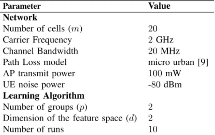
Parameter Value Network
Number of cells (m) 20
Carrier Frequency 2 GHz
Channel Bandwidth 20MHz
Path Loss model micro urban [9]
AP transmit power 100mW
UE noise power -80dBm
Learning Algorithm
Number of groups (p) 2
Dimension of the feature space (d) 2
Number of runs 10
TABLE II: Network and learning algorithm parameters.
0 5 10 15 20 Number of Groups 1.5 2 2.5 3 3.5 Prediction RMSE q=16 q=36 q=64 (a) 0 20 40 60 80 100 Number of Patches 2 2.5 3 3.5 Prediction RMSE m=20 APs m=100 APs (b)
Fig. 6: RMSE of the prediction error of group learning withn= 1000
users vs. number ofpof groups used and numberqof patches used. The sashed lines in plot (a) indicate results with ordinary matrix factorisation. Unless otherwise statedm= 20, p= 2,q = 64. Full ratings matrix used.
That is, we cap the rate at 40Mbps and ensure that the minimum is at least 1Mbps. In the recommender system we
select distance metricd(u, i) = 1when user uis in the patch
Ai andd(u, i) = 0 otherwise.
We begin with a sanity check using the full matrix of ratings for both training and testing (i.e. without a 20% hold-back being used for testing). Fig 6(a) plots the measured RMSE of the prediction error vs the number of groups used by the automatic group learning approach. It can be seen that as the number of groups increases from 1 to 2 there is a sharp drop in the RMSE, as expected. Further, that the RMSE is similar with both automatic group learning and ordinary matrix factorisation. This confirms that both approaches are able to model the full measured ratings matrix (i.e. with no missing observations) fairly well and with similar levels of accuracy. Fig 6(b) plots the RMSE with automatic group learning as the number of patches is increased. Here the full ratings matrix is again observed, with each user rating every AP from every patch so that for 100 patches, 20 APs and 1000 users there
are 100×20×1000 = 2M ratings. It can be seen that the
RMSE falls as the number of patchesqis increased, as might
be expected since more fine grained information becomes
available as q increases. Results are shown for both 20 and
100 APs, and are much the same for both.
We now proceed to consider the impact of missing observa-tions and to evaluate the predictive power of the recommender system for data not used for training i.e. its generalisation
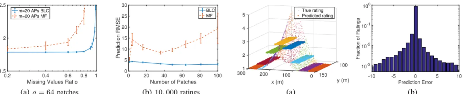
0.2 0.4 0.6 0.8 1 Missing Values Ratio 1.5 2 2.5 Prediction RMSE m=20 APs BLC m=20 APs MF (a)q= 64patches 0 20 40 60 80 100 Number of Patches 0 5 10 15 20 25 30 Prediction RMSE BLC MF (b)10,000ratings
Fig. 7: RMSE of the prediction error vs sparsity of measured ratings available. Data shown both with group learning (indicated as BLC) and ordinary matrix factorisation (indicated as MF). Unless otherwise stated,n= 1000users,m= 20APs,q= 64patches,p= 2groups.
performance. A subset of 20% of the full rating matrix is selected unformly at random without replacement to be held back and used for testing of prediction accuracy. Of the remaining 80% of ratings a subset are selected unformly at random without replacement according to a specified missing values ratio (a missing values ratio of 0.5 corresponding to drawing 50% of these ratings).
Fig 7(a) plots the prediction RMSE as the missing values ratio is varied. Results are shown both with automated group learning and with ordinary matrix factorisation. It can be seen that, similarly to Figure 3(b), when automated group learning is used the RMSE increases much more slowly as the number of missing values increases.
Fig 7(b) shows the prediction RMSE as the number of ratings is held constant and the number of patches is varied. Note that the setup differs from Fig 6(b) not only in that a 20% hold-back is used for testing but also in that the number of ratings is held constant at 10,000 whereas in Fig 6(b) the number of ratings varies with the number of patches used (the
full ratings matrix is of size q×m×n). Hence, in Fig 7(b)
the missing values ratio increases as the number of patches increases. This is closer to the situation in reality, and leads to a trade-off whereby as the patch size is made smaller (i.e. the number of patches is increased) the diversity of ratings for an access point due to location variations can be expected to decrease, tending to improve prediction accuracy, but at the same time the number of observed user ratings in each patch will also tend to decrease, tending to degrade prediction accuracy. As a result, we observe in Fig 7(b) that the RMSE exhibits a minimum. For 10,000 ratings when ordinary matrix factorisation is used the minimum is when the number of
patches is aroundq= 36and when automated group learning
is used the minimum is at aroundq= 64patches. The increase
in the optimum with automated group learning is due to its better performance when ratings are sparse, see Fig 7(a).
We can gain some more insight into the prediction perfor-mance from Figure 8. Figure 8(a) plots the true and predicted
ratings for one example AP as those users withCu= 0move
through a sequence of patches running through the middle of the area considered (the physical locations are indicated by the
xandy axes of the plot). It can be seen that the true ratings
peak around the centre-back of the plot and decrease smoothly
100 y (m) 1 2 3 4 300 x (m) 5 200 100 0 150 True rating Predicted rating (a) -10 -5 0 5 10 Prediction Error 10-3 10-2 10-1 100 Fraction of Ratings (b)
Fig. 8: Comparison of predicted and actual ratings for a representative AP and users located in a single patch (location indicated on thex and y axes). Forn = 1000 users, m= 20 APs, q = 64 patches, p= 2groups and with group learning.
as the distance from the AP increases, in line with the path loss model used. In contrast, within each patch the predicted ratings for users sharing the same group are essentially constant, with this constant value roughly equal to the mean rating of users from that group in that patch. Since the recommender system lacks location information more detailed than the patch in which a user is located, this clearly is a sensible strategy and serves to give some confidence that the recommender system is indeed working in a reasonable fashion.
Figure 8(b) plots the distribution of prediction errors over all ratings (not the RMSE but the error for each individual rating). It can be seen that the errors are concentrated around zero and that the probability of exceeding 2 is less than 1%.
VI. CONCLUSIONS
In this paper we consider user to cell association in a wireless network with multiple access points. We propose use of a recommender system to inform the mapping of users to cells. We demonstrate the effectiveness of the proposed grouped-based user to cell associations for a set of syntheti-cally generated user/cell ratings.
REFERENCES
[1] “Jiwire Hotspot Directory..” http://www.jiwire.com. [2] “FON Wireless..” https://fon.com.
[3] C. Doctorow, “Why hotel wifi sucks,” 2005.
[4] “T-Mobile Germany Blocks iPhone Skype over 3G and WiFi.” http://jkontherun.com/2009/04/06/t-mobile-germany-blocks-iphone-skype-over-3g-too, 2010.
[5] S. Singh, H. S. Dhillon, and J. G. Andrews, “Offloading in heterogeneous networks: Modeling, analysis, and design insights,”Wireless Communi-cations, IEEE Transactions on, vol. 12, no. 5, pp. 2484–2497, 2013. [6] M. Bennis, M. Simsek, A. Czylwik, W. Saad, S. Valentin, and M.
Deb-bah, “When cellular meets wifi in wireless small cell networks,” IEEE Communications Magazine, vol. 51, no. 6, pp. 44–50, 2013.
[7] J. Pang, B. Greenstein, M. Kaminsky, D. McCoy, and S. Seshan, “Wifi-reports: Improving wireless network selection with collaboration,” IEEE Transactions on Mobile Computing, vol. 9, no. 12, pp. 1713–1731, 2010. [8] A. Checco, G. Bianchi, and D. Leith, “Blc: Private matrix factorization recommenders via automatic group learning,” ACM Trans Security and Privacy, 2017.
[9] 3GPP TR 36.819 V11.1.0 (2011-12) Technical Specification Group Radio Access Network; 3rd Generation Partnership Project; Coordinated multi-point operation for LTE physical layer aspects (Release 11), 2011.