University of Arkansas, Fayetteville
ScholarWorks@UARK
Theses and Dissertations8-2012
Socio-Demographic and Economic Determinants
of Food Deserts
Zhongyi Wang
University of Arkansas, Fayetteville
Follow this and additional works at:http://scholarworks.uark.edu/etd
Part of theDemography, Population, and Ecology Commons
This Thesis is brought to you for free and open access by ScholarWorks@UARK. It has been accepted for inclusion in Theses and Dissertations by an authorized administrator of ScholarWorks@UARK. For more information, please contactscholar@uark.edu, ccmiddle@uark.edu.
Recommended Citation
Wang, Zhongyi, "Socio-Demographic and Economic Determinants of Food Deserts" (2012).Theses and Dissertations. 562.
SOCIO-DEMOGRAPHIC AND ECONOMIC DETERMINANTS OF FOOD DESERTS
A thesis submitted in partial fulfillment of the requirements for the degree of Master of Science in Agricultural Economics
By
Zhongyi Wang
Chongqing Technology and Business University Bachelor of Science in Economics, 2008
August 2012 University of Arkansas
ABSTRACT
In this paper we utilized a panel data set from 2004 to 2010 to identify and determine the demographic and economic drivers of food deserts in both urban and rural areas in Arkansas. We defined food deserts as areas where access to healthy foods such as fresh vegetables and fruits are limited. More specifically, separate distance measures from the census block centroid to the nearest supermarket or grocery store were used to determine if the area is an urban food desert (1 mile) or rural food desert (10 miles). These distance measures were then aggregated at the census block group level. Locations of supermarkets and big grocery stores that provide fresh produce were geocoded (latitude and longitude) accordingly. Socio-demographic and economic variables at the census block group level were then matched with the distance information. These variables were from Census 2000 Summary File 3. Finally, we employed multivariate regression approaches to model the relationship between socio-demographic and economic factors and the existence of urban and rural food deserts in Arkansas. We found that block groups with deprived situation, such as less per capita income, higher unemployment, and less educational attainment, will be more likely to be food deserts.
This thesis is approved for recommendation to the Graduate Council.
Thesis Director: _______________________________________ Dr. Rodolfo M. Nayga, Jr. Thesis Committee: _______________________________________ Dr. Michael Thomsen _______________________________________ Dr. Bruce L. Dixon
THESIS DUPLICATION RELEASE
I hereby authorize the University of Arkansas Libraries to duplicate this thesis when needed for research and/or scholarship.
Agreed _________________________________________ Zhongyi Wang
Refused __________________________________________ Zhongyi Wang
ACKNOWLEDGMENTS
I would like to mention some people who gave me help, support and encouragement during the whole process of writing my thesis. First, thanks go to my parents who have encouraged me and invested in my education. Second, special thanks are due to the director of my thesis
committee member, Dr. Rodolfo M. Nayga, Jr., and other two committee members, Dr. Michael Thomsen and Dr. Bruce L. Dixon for all of their help and good advice with thesis. It would be impossible to make it through the whole process without their help.
Additionally, special thanks also go out to the staff of Department of Agricultural Economics and Agribusiness at the University of Arkansas, especially Pedro A. Alviola IV, Diana Danforth, Jim Smartt. Their comments, review were also very constructive and very much appreciated. Thanks also go to my fellow master degree student, Jiao Yucong, who has helped me a lot with the thesis. Special thanks also go to Dr. Lucas Parsch for his advice and dedication to students. I acknowledge, also, my other fellow students who have made my graduate life enjoyable.
CONTENTS
INTRODUCTION ... 1
DATA ... 6
Study Area ... 6
Food Store Data ... 7
Demographic and Socioeconomic Data ... 9
Regional Data ... 13
METHODOLOGY ... 15
Definition of Urban and Rural Blocks ... 15
Definition of Urban and Rural Block Groups ... 15
Food Store Locations in Urban and Rural Block Groups ... 16
Measuring Food Access ... 19
Low Income Block Groups ... 20
Identification of Food Deserts ... 21
MODEL SPECIFICATION ... 32
RESULTS ... 35
Random Effects Linear Regression ... 35
Random Effects Logistic Regression ... 37
Year by Year Logistic Regression... 37
DISCUSSION AND CONCLUSION ... 45
1 INTRODUCTION
The concept of a “food desert” was first used in Scotland in the early 1990s (Cummins and Macintyre 1999) but during that time there was no commonly accepted definition of the concept. Recently, food deserts have been defined as urban areas where people do not have access to an affordable and healthy diet (Cummins and Macintyre 2002). On the other hand, former UK Health Minister Tessa Jowell broadened the definition of food deserts as areas “where people do not have easy access to healthy, fresh foods, particularly if they are poor and have limited mobility” (Furey, Strugnell, and McIlveen 2001). Some of the initial studies focused on the food environment in the urban areas (Alwitt and Donley 1997; Zenk et al. 2005), but later on researchers observed that rural areas also contain food deserts (Blanbard and Lyson 2006; Hendrickson, Smith, and Eikenberry 2006; McEntee and Agyeman 2010).
In this paper, both rural and urban areas in Arkansas were included in the analysis. The rural and urban blocks were defined according to the urban places found in the 2000 and 2010 Census. The urban places are geographical units which are composed of blocks. If a block is located in urban places, then that block is defined as an urban block. A rural block is an area which does not belong to any urban places. This study identified both rural and urban food deserts in Arkansas. Several studies including McEntee and Agyeman (2010) investigated the whole state of Vermont using the same food desert identification criteria since they assumed Vermont is largely a rural state. Kaufman (1999) evaluated some rural counties in the Lower Mississippi Delta area while other researchers evaluated food deserts in a specific urban city setting (Apparicio, Cloutier, and Shearmur 2007; Wrigley 2002; Sparks, Bania, and Leete 2009).
Arkansas has not been studied before as a whole state, although the Lower Mississippi Delta area research included a few areas of Arkansas.
In general, food deserts are areas where residents have limited access to healthy foods. Thus the definition of food deserts entails the elaboration of two concepts, namely the nature of limited access and sources of healthy food. Researchers have developed several methods in defining limited access. These methods can be summarized into two categories; First is the measurement of the density within a community (Clarke, Eyre, and Guy 2002; Block, Scribner, and Desalvo 2004; Blanchard and Lyson 2006; Berg and Murdoch 2008; Apparicio, Cloutier, and Shearmur 2007; Alwitt and Donley 1997) and second is the calculation of the distance to food stores (Algert, Agrawal, and Lewis 2006; Apparicio, Cloutier, and Shearmur 2007; Sharkey and Horel 2008; Morton and Blanchard 2007; Short, Guthman, and Raskin 2007; McEntee and Agyeman 2010). When using the density measure, researchers count the number of food stores within a specific radial distance. For example, Apparicio, Cloutier, and Shearmur (2007) measured the number of supermarkets within 1000 meters of a block centroid. Likewise, Berg and Murdoch (2007) counted the stores that are within a 1-mile radius at the census block group level whereas Alwitt and Donley (1997) examined the number of retail stores in zip codes. In the distance calculation method, the Geographic Information System (GIS) is used to measure the distance to the nearest food store. Studies using this approach have measured the distance from the residential units to the supermarkets and calculated the distance to the nearest food store from the population-weighted center of each Census Block Group (McEntee and Agyeman 2010; Sharkey and Horel 2008).
3
The identification of low access areas differs for both rural and urban areas. For the rural areas, in Morton and Blanchard’s (2007) study, they measured food access at county level in rural America. If 50 percent of the population in a county resides more than 10 miles from a large food store, then the county was identified as a low access area. If all residents in one county live more than 10 miles from a large food store, then that county was defined as a food desert. In Blanchard and Lyson’s (2006) study, they examined food deserts in nonmetropolitan South of U.S. Low access was defined for people to travel 10 miles to a supermarket. A county was classified as a food desert if half or more of the population has low access to supermarkets. McEntee and Agyeman (2010) identified rural food deserts at Census Tract level in the state of Vermont. They used 10 mile distance from residential units to food retailers to define food deserts directly without defining low access first. For the urban areas, the study by Algert, Agrawal, and Lewis (2006) measured access using distance from a store offering fresh produce in Los Angles. Those living outside of 0.8 km or about a 15 minute walk were highlighted as not having access to a variety of produce. In Apparicio, Cloutier, and Shearmur’s (2007) study, they set 1 kilometer to the nearest supermarket to be the criterion of defining low access. In the USDA/ERS 2009 Report, 1 mile was used to determine low access. If the distance to the nearest supermarket is less than 0.5 mile, high access was defined. Medium access was defined to be between 0.5 and 1 mile.
In our research study, the 10 mile and 1 mile thresholds were used as the criteria for defining limited access in rural and urban areas respectively. The distance was calculated from the block centroid to the nearest food store. The block level was used because the block is the
smallest geographical unit in the census and it can better capture the community food store environment. Then low access was defined at the block group level, where the block group is comprised of several blocks. According to the USDA/ERS’ Food Desert Locator definition, if 33% or more population in a Census Tract reside more than 1 mile from a supermarket or a large grocery store, then the Census Tract is defined as low access. For rural Census Tract, the distance is set to be more than 10 miles. We modified the Census Tract to Block Group, since our study was based on the block group level and those socio-demographic and economic factors were obtained from Block Group level.
Several studies have selected supermarkets or big grocery stores as food sources where residents can purchase healthy foods (Sparks, Bania, and Leete 2009; McEntee and Agyeman 2010; USDA Report 2009; Apparicio, Cloutier, and Shearmur 2007; Baker et al. 2006). For example, McEntee and Agyeman (2010) selected food retailers according to the North
American Industry Classification System (NAICS) number. Stores larger than 2500 square feet were selected if the NAICS number is 44511, which indicates “Supermarket and other Grocery”. They utilized the food store size in order to filter out convenience stores and gas stations. Also, Sparks, Bania, and Leete (2009) used the NAICS to obtain food store data in their analysis. Other studies defined food stores as stores operating under the mainline chain grocery stores in their study area (Berg and Murdoch 2008). In this paper, the Standard Industry Code (SIC) was used to determine the food store categories that were relevant. The criterion used is whether the food store provides fresh produce. The food store location data were obtained from Dun and Bradstreet (D&B).
5
While several studies used distance in defining food deserts, others also considered factors related to social and economic issues. For example, Guy, Clarke, and Eyre (2004) measured the spatial distribution of food stores and considered areas with high deprivation as food deserts. The high deprivation measure/index was calculated using data pertaining to income,
employment, and education. Apparicio, Cloutier, and Shearmur (2007) also included low income population and social deprivation index to examine the association with accessibility to supermarkets. The social deprivation index considered such factors as single-parent families, unemployment rate, and adults with low level of schooling. In Sparks, Bania, Leete’s (2009) study, they defined food deserts as high poverty areas (Census tract with poverty rates at 20 percent or higher) that have low or very low access to supermarkets. In the identification of food deserts, this study followed the USDA/ERS definition mentioned earlier. Hence, besides the low access criteria, this research also considered income as a factor in identifying food deserts. Low income areas were identified at block group levels. These are all discussed in detail in the methodology section. From the past food deserts studies, some only examined the different methods to identify the food deserts in certain areas and did not relate the food deserts areas with the community socio-demographic and economic characteristics(Blanchard and Lyson 2006; Morton and Blanchard 2007; McEntee and Agyeman 2010; Sparks, Bania, and Leete 2009). Other studies examined the food access/environment in some communities and their association with neighborhood characteristics (Kaufman 1999; Algert, Agrawal, and Lewis 2006; Morland and Filomena 2007; Berg and Murdoch 2008; Sharkey and Horel 2008). But these studies only measured the access and did not define food deserts. Thus, the objective of
this study is to identify the food deserts areas and determine the various community
demographic and socioeconomic factors that are likely to be associated with food desert areas. Another contribution of this study is that it includes rural and urban areas for the whole state of Arkansas. In addition, this study aims to identify food deserts across 7 years from 2004 to 2010 using a panel data structure which previous studies have not utilized.
The next section discusses the data and methodology used in the identification of food deserts. This includes the rural and urban definition and the low access and low income block group identification. The paper then presents the results and discusses the conclusions. DATA
Study Area
The focus of this study is on Arkansas, a predominantly rural state with a population of 2,915,918 and with a land area of approximately 33,287,812 acres. Farmland accounts for 41.7% of the state’s land, while rural population is almost 40 percent of the total population (USDA Economic Research Service, 2011). Food deserts are not only a problem for urban cities because in rural areas, residents sometimes need to drive longer distances to purchase healthy food. This study conducted analysis in both rural and urban areas in the state. Arkansas has a higher disadvantaged population, for example, people with bachelor degree or higher is only 19.1 percent which is lower than the average 27.9 percent across the country. Per capita income of one year is $21,274 which is also lower than the national average of $27,334. Median
household income is $39,267, and the national average is $51,914 which is much higher than the Arkansas. Percent of persons below poverty level is 18 which is higher than U.S. average of
7
13.8 (2010 Census). In terms of the obesity rates, Arkansas is among states with adult obesity rates over 30 percent, which is the highest category (Centers for Disease Control and
Prevention 2010). Food Store Data
This analysis used food stores that offer fresh fruits and vegetables. Consumption of fresh produce is an integral component of maintaining a healthy diet. The study assumed that food stores with a fresh produce department have the capacity to provide other types of food since food stores that have a produce department are typically large grocery stores like supermarkets. The 2004 to 2010 data on food store outlets were obtained from a business list developed by Dun and Bradstreet (D&B).The information contained in the dataset enabled the sorting of stores by multiple criteria such as the name, address, annual sales, and Standard Industry Classification (SIC) codes of business types.
The SIC codes were used to create the list of food stores in the analysis. Food store outlets are categorized based on the following types: (1) department stores-discount (SIC: 53119901), (2) warehouse club stores (SIC: 53999906), (3) supermarkets (SIC: 54110100), (4) chain supermarkets (SIC: 54110101), (5) independent supermarkets (SIC: 54110103), (6) grocery stores (SIC: 54110000), (7) chain grocery stores (SIC: 54119904), (8) independent grocery stores (SIC: 54119905), and (9) health foods store (SIC: 54990100 and 54990102).
Previous studies classified grocery stores in different ways. For example, one study selected food retailers with the size of a food store equal to or greater than 2500 square feet (McEntee and Agyeman 2010) while Morton and Blanchard (2007) chose stores with 50 or
more employees. On the other hand, Kaufman (1999) used the criteria of $500,000 annual sales to filter out small grocery stores based on the sales criteria set by the Food and Nutrition
Services, USDA. This study applied and modified Kaufman’s (1999) sales criterion where grocery stores with annual sales greater than $400,000 were selected. Our justification in the present study to include grocery stores with sales equal or greater than $400,000 is to avoid deleting stores that provide fresh produce even though the sales are less than $500,000.
To further justify the $400,000 criteria, phone calls were made to individual stores which have annual sales in the range of $400,000 to $500,000.During the phone interview, the stores were asked if they consider themselves a full-service grocery store with a full produce
section/department. A total of 14 stores in the database are within the $400,000 to $500,000 sales range. Eleven out of these 14 stores were contacted and five of the 11 stores have fresh produce sections and two stores offer a small fruit and vegetable section. To further examine this issue for stores with less than $400,000, random selection was performed in some of these stores to make sure if they offer fresh produce. It was found that none of the stores with annual sales of less than $400,000 offer fruits and vegetables except a few chain grocery stores. We kept those chain grocery stores because they do provide fresh produce, although their annual sales are under $400,000. These chain grocery stores are just a few exceptions. The sales criterion of $400,000 was still chosen for the analysis.
A shortcoming of using the sales information is that there are some stores with missing sales information. This was addressed by checking each company name to make sure if they are indeed a supermarket or a large grocery store. Since most of the stores with missing sales
9
information are chain supermarkets and chain grocery stores, the stores’ websites were examined to determine if the stores offer fresh produce. Thus, in validating the data set, every food store was checked in the list and those which are not supermarkets or grocery stores like gas stations, convenience stores and restaurants were deleted. With this process, a total of 564, 577, 589, 566, 586, 486, and 496 food stores were identified each year from 2004 to 2010, respectively.
Demographic and Socioeconomic Data
There are past studies (Morland et al. 2002; Morland and Filomena 2007; Powell, Chaloupka, and Bao 2007) that utilized the Census data to capture community characteristics. In this study, the demographic and socioeconomic measures at the Block Group level were obtained from the 2000 Census Summary File 3 (SF-3).The SF-3 contains the Census 2000’s social, economic and housing characteristics compiled from a population sample and housing units. The information on population includes total population, urban and rural data, households and families,
occupation, income and others. On the other hand, the housing information included basic housing totals, urban and rural information, number of rooms, vehicles available, value of home, monthly rent and others. The information regarding the Census Block Group characteristics used in the analysis include urban blocks within a Block Group, population, race, age, length of journey to work (commuting time), types of transportation to work, employment status,
educational attainment, and income and poverty rates. Table 1 shows the summary statistics for the census variables used in this study. All the units of variables were modified to meet the model analysis. Most of the variables were measured in proportion. Income and population variables
were measured at one thousand units. We can see that average proportion of people driving car to work is 0.93, which is very high. Average proportion of people with high school education or higher is 0.73, which is also not bad. But the per capita income is a little bit low, averaged around 16,000 USD. People below poverty, another economic index, averaged at 0.18, which is not low. The proportion of urban blocks within block groups is also very low, reaching an average of 0.21.
Table 1. Descriptive Statistics for Census Variables (N=2135)
Variable Definition Unit Mean Std.Dev. Min Max
age18_prp people less than or equal to 18 Proportion 0.266805 0.065687 0.000 0.570957
age19to39_prp people with age between 19 and 39 Proportion 0.285273 0.091272 0.000 1
age40to64_prp people with age between 40 and 64 Proportion 0.300314 0.071036 0.000 1
age65gt_prp people equal to or greater than 65 Proportion 0.146671 0.077704 0.000 0.747253
commute30_60min_prp people commute between 30 and 60 minutes Proportion 0.20285 0.132741 0.000 0.726655
commute30min_prp people commute less than 30 minutes Proportion 0.71591 0.162018 0.000 1
commutegt60min_prp people commute greater than 60 minutes Proportion 0.054265 0.04695 0.000 0.39934
drivecartowork_prp people who drive car/truck/van to work Proportion 0.931732 0.071349 0.000 1
othertowork_prp people who use other means to work Proportion 0.041369 0.054671 0.000 0.653061
workathome_prp people working at home Proportion 0.025102 0.026296 0.000 0.2
gthighschool_prp people receiving high school or higher Proportion 0.730715 0.126185 0.000 1
lthighschool_prp people not receiving high school Proportion 0.26788 0.12358 0.000 1
inlabor_prp people in labor force Proportion 0.594887 0.107023 0.000 0.988877
notinlabor_prp people not in labor force Proportion 0.404176 0.106184 0.000 1
ltpov_prp people below poverty Proportion 0.175463 0.121232 0.000 1
hispanic_prp Hispanic or Latino Proportion 0.029435 0.057571 0.000 0.566667
nonhispanic_prp not Hispanic or Latino Proportion 0.969629 0.064773 0.000 1
white_prp white Proportion 0.766215 0.276262 0.000 1
nonwhite_prp non-white Proportion 0.233067 0.275393 0.000 1
nopubasstinc_prp households w/o public assistance income Proportion 0.965384 0.060892 0.000 1
pubasstinc_prp households w/ public assistance income Proportion 0.031806 0.032909 0.000 0.340206
pcinc_scale Per capita income (1000 dollars) count 16.26335 6.22973 0.000 72.657
poptotal_scale sum of population in all blocks (1000 people) count 1.252178 0.650636 0.000 6.558
urbanblk_prp urban blocks Proportion 0.218786 0.40168 0.000 1
13 Regional Data
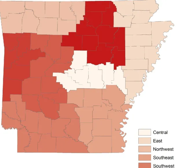
In addition to the census variables, regional variables were also included in the analysis. We used the Arkansas Planning and Development Districts. The information was obtained from the official website of Arkansas state. In their classification, Arkansas is divided into eight planning and development districts. Each district covers six to twelve counties which tend to have common economic structures and opportunities. They are important in economic planning and development process at the local level. In addition to assessing the economic development for each area, the district also acts as intermediary whom counties interact with economic development offices of the state and federal governments. These districts have been the major channels for funds of development programs in Arkansas. The eights districts are Central Arkansas, East Arkansas, Northwest Arkansas, Southeast Arkansas, Southwest Arkansas, West central Arkansas, Western Arkansas and White River. These districts were coded as indicator variables at block group level. Since these districts are comprised of counties and counties are made up of block groups. The districts map is shown in Figure 1.
14
15 METHODOLOGY
A number of past studies have used different measures in determining food access. In some cases, mail surveys were used to obtain information (Hendrickson, Smith, and Eikenberry 2006). However in some studies (Morton and Filomena 2007; Sharkey and Horel 2008) food access measures were derived by calculating the distance from the centroid of an area (e.g. zip code, census tract, or block) to the nearest food store. Since distances in sparsely populated areas are often not directly comparable to distances in densely populated areas, many studies have separated the analysis of rural and urban food access (USDA report 2009).
Definition of Urban and Rural Blocks
In this study, the analysis was conducted at the census block group level. Since there are corresponding Census socio-demographic characteristics at the block group level, the study was able to analyze the association between food deserts and the community food environment factors. The distance was measured at block level and was aggregated to block group level using the population weighted method. The definition of urban and rural areas was based on the blocks, because urban and rural block groups are not defined according to the Census rural and urban definition. The urban and rural blocks were defined using the Census defined urban places. The census defined urban places are composed of blocks. From this information, the blocks which are in the urban defined places are considered urban while the blocks not in urban defined places are considered rural blocks.
Definition of Urban and Rural Block Groups
16
could not find an official definition of block groups. As mentioned earlier, block groups are made up of blocks, and we know the total number of blocks within a block group. The urban/rural blocks were also known, and then the percentage of urban or rural blocks can be calculated. We calculated the percentage of urban blocks within a block groups. We defined the block groups with 0 percentage of urban blocks as rural block groups and blocks groups with 100 percentage of urban blocks as urban block groups. There are 2135 block groups in total. After the classification, 1991 block groups were with 0 or 100 percentage of urban blocks. 1601 block groups were defined rural with 0 percentage of urban blocks, and 390 block groups were classified as urban with 100 percentage of urban blocks. The remaining 144 block groups were unclassified. The 144 block groups were excluded in the separate model analysis of urban and rural block groups. It is a small proportion to the whole block groups.
Food Store Locations in Urban and Rural Block Groups
Previous study about the food store location has been examined. In Morland et al. (2002), they evaluated the association of food store location with neighborhood characteristics. They found that more food stores are located in wealthier neighborhood and more supermarkets are in the white neighborhood. This paper aims at analyzing food deserts in urban and rural areas. Therefore, we plotted a map containing the food store in urban and rural block groups. The following Figure 2 and Figure 3 show this information.
17 Figure 2. Food Stores Locations within Arkansas
18
19
We cannot see the black urban block groups in Figure 2, since the urban ones constitute a small percentage of the total block groups. Urban block group usually have smaller area compared to rural ones. Therefore, Figure 3 shows the zoom in picture of an urban area around Little Rock. We can see from figure that urban block groups have higher density of food stores. Measuring Food Access
The methods that were developed in previous studies to measure food access vary considerably (Furey, Strugnell, and McIlveen 2001; Algert and Agrawal 2006; Alwitt and Donley 1997; Apparicio, Cloutier, and Shearmur 2007; Berg and Murdoch 2008; Clarke, Eyre, and Guy 2002). These methods include emailing out questionnaires and performing surveys in order to obtain information (Furey, Strugnel, and McIlveen 2001). More recently, however, researchers have been using the Geographic Information System (GIS) in compiling
quantitative data in order to measure food access. The commonly used measures of accessibility found in the literature are the distance to the closest food store and the number of stores within a certain distance radius. The distance to the nearest food retailer can be measured from the centroid of a geographical area, such as block or block group. And it can be measured in a straight line or a road network distance. For the number of food retailers, researchers usually set a specific radius and count the food store number and some criteria are used to determine which number of food stores should be identified as low access. Previous food desert studies (Clark, Eyre, and Guy 2002; Smoyer-Tomic, Spence, and Amrhein 2006; Larsen and Gilliland 2008) used multiple measures to evaluate access. These include distance to the nearest supermarket,
20
the number of supermarkets within a walkable distance of less than a kilometer and the mean distance to three supermarkets (Apparicio, Cloutier, and Shearmur 2007). In this study, the distance from the block centroid to the nearest food store was used as a measure of food access. The reason for the usage of the block centroid is that the rural and urban areas are determined at the block level. Since the block level is the smallest unit in the census, it can better capture the food store environment within the communities. Using food store data from 2004 to 2010, food access measures were calculated for Arkansas.
Other studies have also used different criteria in classifying low access in urban areas. For instance, Apparicio, Cloutier, and Shearmur (2007) used a kilometer as the distance threshold in classifying low access, while the USDA-ERS (2009) used the one mile cut-off. This study follows the USDA/ERS approach. For rural areas, the 10 mile cut-off was chosen as the
threshold similar to the approach used by McEntee and Agyeman (2010) and Morton and Lyson (2007). Distances were measured from the block centroid to the nearest food store. Blocks whose distance from the nearest food store were greater than 1 mile and 10 miles are defined as “low access” in urban and rural areas, respectively. The low-access population was then
summed from the block level to the block group level in order to obtain the percentage of population that is low food access. If at least one third of the population is classified as low access at the block group level, then the block group was classified as “low access”.
Low Income Block Groups
As part of the criteria in identifying food desert block groups, the block group must also be classified as a low income area in addition to being a low access area. In this case, the study
21
followed the USDA/ERS criteria in defining a low income area. Following the USDA/ERS definition, the criteria includes: 1) 20% or more of the block group population was below poverty; 2) for block groups located within a metropolitan statistical area (MSA), the median family income for the block group does not exceed 80 percent of statewide median family income; 3) for block groups located within a non-metropolitan statistical area (NMSA), the median family income for the block group does not exceed 80 percent of the greater of
statewide median family or the metropolitan area median family income. If any of these criteria applied to a block group, then the block group was classified as a low income area.
Identification of Food Deserts
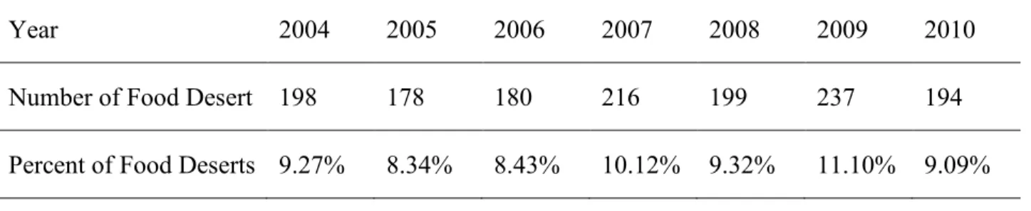
After determining which block groups were considered low access and low income, a block group is then classified as a food desert if it is both a low income area and at least 33 percent of the population in the block group have low access to a food store that offer fresh produce. This criterion resulted in 198 block groups for 2004; 178 and180 block groups for 2005 and 2006; 216, 199, and 237 block groups for 2007 to 2009; and 194 block groups in 2010. The food deserts maps for the 7 years are listed from Figure 3 to Figure 9. Some statistics about the food deserts across years are presented in the following Table 2, Table 3, and Table 4.
Table 2. Food Deserts across Years for all Block Groups (N=2135)
Year 2004 2005 2006 2007 2008 2009 2010
Number of Food Desert 198 178 180 216 199 237 194
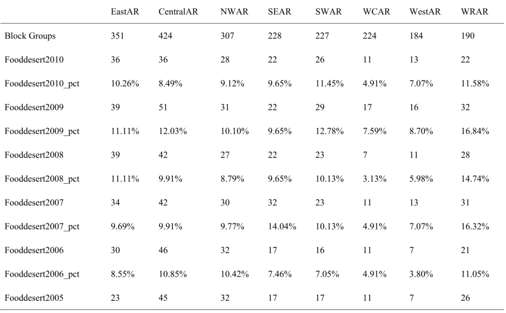
Table 3. Food Deserts by Districts across Years for All Block Groups (N=2135)
EastAR CentralAR NWAR SEAR SWAR WCAR WestAR WRAR
Block Groups 351 424 307 228 227 224 184 190 Fooddesert2010 36 36 28 22 26 11 13 22 Fooddesert2010_pct 10.26% 8.49% 9.12% 9.65% 11.45% 4.91% 7.07% 11.58% Fooddesert2009 39 51 31 22 29 17 16 32 Fooddesert2009_pct 11.11% 12.03% 10.10% 9.65% 12.78% 7.59% 8.70% 16.84% Fooddesert2008 39 42 27 22 23 7 11 28 Fooddesert2008_pct 11.11% 9.91% 8.79% 9.65% 10.13% 3.13% 5.98% 14.74% Fooddesert2007 34 42 30 32 23 11 13 31 Fooddesert2007_pct 9.69% 9.91% 9.77% 14.04% 10.13% 4.91% 7.07% 16.32% Fooddesert2006 30 46 32 17 16 11 7 21 Fooddesert2006_pct 8.55% 10.85% 10.42% 7.46% 7.05% 4.91% 3.80% 11.05% Fooddesert2005 23 45 32 17 17 11 7 26 22
Fooddesert2005_pct 6.55% 10.61% 10.42% 7.46% 7.49% 4.91% 3.80% 13.68%
Fooddesert2004 23 58 35 17 17 11 9 28
Fooddesert2004_pct 6.55% 13.68% 11.40% 7.46% 7.49% 4.91% 4.89% 14.74%
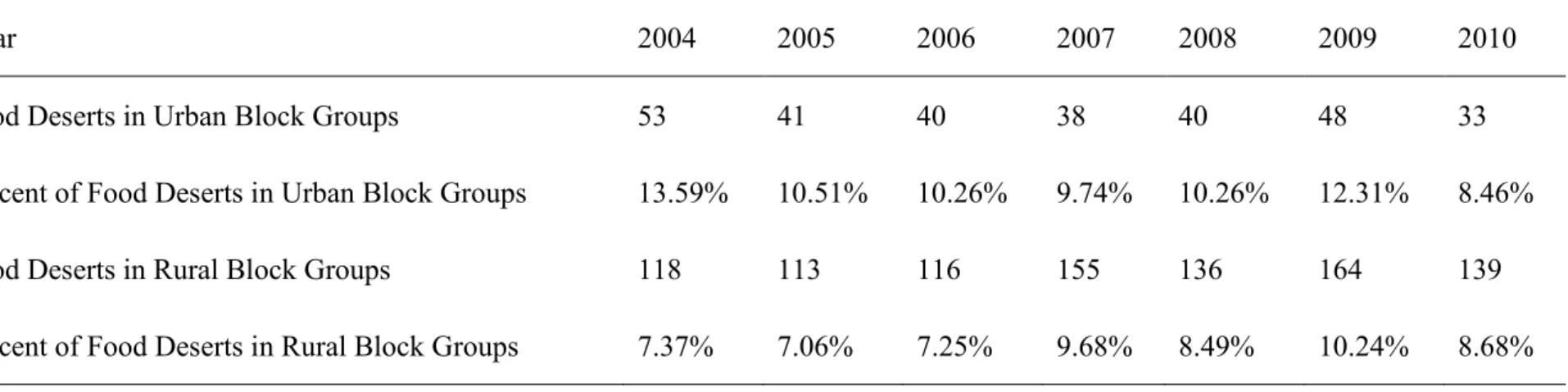
Table 4. Food Deserts across Years for Defined Urban and Rural Block Groups (N=1991)
Year 2004 2005 2006 2007 2008 2009 2010
Food Deserts in Urban Block Groups 53 41 40 38 40 48 33
Percent of Food Deserts in Urban Block Groups 13.59% 10.51% 10.26% 9.74% 10.26% 12.31% 8.46%
Food Deserts in Rural Block Groups 118 113 116 155 136 164 139
Percent of Food Deserts in Rural Block Groups 7.37% 7.06% 7.25% 9.68% 8.49% 10.24% 8.68%
24
In Table 2, the percentage of food deserts in 2009 is the highest. It may be explained by the economic recession in that year. The number of food store is also the lowest in 2009 compared to other years. Food deserts in the 8 districts were also shown in Table 3, it can be observed that White River district has the highest percentage of food deserts across all years. Therefore, the White River region was set to be the base variable in the following model analysis. In addition, the number of food deserts was also calculated separately for urban and rural block groups. It can be noted that the highest percentage of food deserts for rural block groups is also in 2009, but it is not for urban block groups. The highest one for urban block groups is in 2004.
25 Figure 3. Food Deserts in 2004
26 Figure 4. Food Deserts in 2005
27 Figure 5 Food Desert in 2006
28 Figure 6. Food Deserts in 2007
29 Figure 7. Food Deserts in 2008
30 Figure 8. Food Deserts in 2009
31 Figure. 9 Food Deserts in 2010
32 MODEL SPECIFICATION
In this study, both the random effects linear regression and the logistic panel models were used to measure the association between food deserts areas and the demographic and
socioeconomic characteristics at block group level for all block groups, urban block groups, and rural block groups. The panel regression model was used to examine the relationship between distance (a continuous variable) and socio- demographic characteristics affecting the distance measure. On the other hand, the panel logistic model measured the effects of various
demographic and socio-economic factors on the likelihood of a block group being a food desert. Probit model was also tried to see if it generated similar results to Logistic model. However, all the marginal effects generated by Probit are insignificant. So the probit model was not included in the final analysis. The general panel structure can be represented as:
(1) Yit= αi + βXit + uit,
Where the subscripts i and t denotes the block group cross section dimension and time period.
Yit represents the dependent variable, while Xit is a vector of independent variables associated
with the response variable Yit. The variable αi is the unobserved time-invariant effects and uitis
the scalar disturbance term.
The elimination of the unobserved time-invariant variable αi is addressed by employing a
fixed effects model. The estimates generated by the fixed effects model use only
within-individual differences, which essentially discards any information about differences between individuals. If the predictor variables vary greatly across individuals but have little variation over time for each individual, then the fixed effects estimates will be imprecise and
33
have large standard errors. In this study, most of the predictor variables are time-invariant because the 2000 Census data values are fixed across the time period. Given our objective of determining the factors that are significantly associated with food desert areas and the time-invariance of a good number of these factors, the analysis is centered on estimates generated by the random effects model.
The rationale behind the random effects model is that, unlike the fixed effects model, the variation across entities is assumed to be random and uncorrelated with the predictor or
independent variables. An advantage of using the random effects model is that one can estimate the coefficients of time-invariant variables. In the fixed effects model, the time invariant
variables are absorbed by the intercept. The random effects model assumes that the error term is not correlated with the predictors which consequently allows for the identification of
time-invariant variables. The baseline empirical models can be specified as: (2) Dit=αi + β1Xit + γZit+uit,,
where the variable Dit represents the population weighted mean distance at the ith block group in t periods (t=2004 to 2010). It is calculated at each block group using the total population of each block within that block group level. Although food deserts are not determined directly based on this distance, it can give us a specific number of mean distance to the nearest food store at each block group level. Xit is a vector of demographic and socioeconomic factors
predicting distance while Zit is a vector of dummy variables representing the geographic district
classifications in Arkansas. A sandwich estimator of the error covariance would was employed to test the heteroscedasticity using STATA software.
34
A panel logistic model was also used in estimating the effects of socio-demographic factors on the likelihood of a block group becoming a food desert. Consider the logistic model as: (3) 𝐿𝑛 1−𝑃𝑖𝑡(𝐹𝐷𝑖𝑡=1)𝑃𝑖𝑡(𝐹𝐷𝑖𝑡=1) =αi + βXit,
where FDit is the response variable for individual i at time t, and takes on the values of either 0
or 1. Let Pit be the probability that FDit=1. By modifying equation 3, the empirical baseline
logistic model can be represented as: (4) 𝐿𝑛 1−𝑃𝑖𝑡(𝐹𝐷𝑖𝑡=1)𝑃𝑖𝑡(𝐹𝐷𝑖𝑡=1) =αi + β1Xit+ γZit,
where FDit is a binary indicator variable denoting whether a block group is a food desert or not. Xit is a vector of socio-demographic variables that are associated with the likelihood of a block
being a food desert and Zit is a vector of regional district indicator variables used in the analysis.
Since most of the predictor variables are time-invariant, the random effects logistic model was used in the analysis.
The above analysis included all the 2135 block groups. Separate analysis was also
conducted for 390 urban block groups and 1601 rural block groups. To do this, we can examine the difference between urban and rural areas.
35 RESULTS
For the state of Arkansas, we identified rural and urban census blocks. There are total 65536 blocks, 62641 blocks are rural areas and 2895 blocks are urban according to the urban places Census definition. Three kinds of model analysis results were presented in the following. In the separate analysis of urban and rural block groups, the percentage of urban blocks variable was excluded, since it was used to control the urban and rural for all block group analysis. It was not needed to be included in the separate analysis. Regional indicators of West Arkansas and West Central Arkansas were deleted due to collinearity.
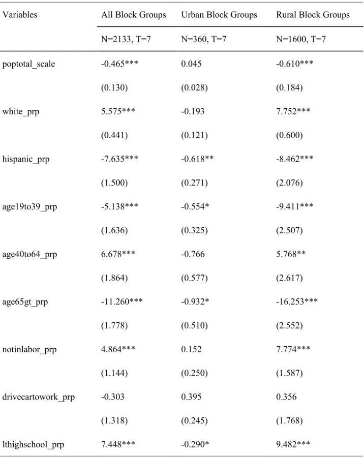
Random Effects Linear Regression
In examining the effects of the socio-demographic factors on the distance to the nearest food store, the comparison of results was presented in Table 5. It can be seen that the rural block groups generated similar results to the all block groups analysis. Most of the coefficients for continuous variables in the rural block groups are greater than the ones in the all block groups.
This study finds that most of the predictor variables were statistically significant except in the urban block group’s model. It may come from its relatively small sample size. For example, if the total population in a block group increases by 1000, the population-weighted distance to the nearest store will decrease approximately by 0.465 miles. This finding is likely to be valid since food stores open in the areas with high concentration of residents. The proportion of white people increase by one unit, the distance will increase by 5.575. The proportion of Hispanic people increase by one unit, distance will decrease by 7.635. For the age groups, if more people
36
with age between 19 and 39 live in a block group, their distance to the nearest food store decreases. And more people with age between 40 and 64 in a block group, the distance will increase. When the age group becomes older, the distance decreases again. It may be explained that elder people tend to choose live in a community which provides convenient life, including close distance to food store. In addition, a one point increase in the proportion of population not in labor force increases the distance by 4.86 miles. In this case, areas with high unemployment rates may on the average translate to lower income and purchasing power. Thus, food stores are unlikely to open in these areas. Also, as per capita income increases by $1000, the distance decreases by approximately 0.08 miles. The reason is that people with more income will purchase more. The proportion of higher people with less than high school education in a block group will also have the distance increased. It makes sense since higher education is positively related to higher income. Holding other things constant, a one point increase in the proportion of urban blocks decreases the distance by approximately 1.395 miles. In this case it might be that more food stores are clustered in urban areas relative to rural areas.
The coefficients for the regional variables are all significant except Southwest district in the all block groups analysis. There are less significant variables in the rural block group’s one. The base district is White River as mentioned before. White River district has the greatest
percentage of food deserts in each year. For the significant regional indicators, the coefficients are all negative, which indicates the distance to the nearest food store is lower for the block groups located in east, southeast, central, northwest, west central and west districts relative to the block groups in the white river district.
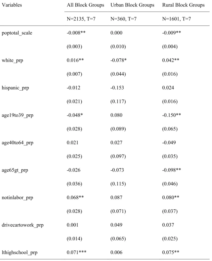
37 Random Effects Logistic Regression
In the panel logistic model, similar results (Table 6) were found relative to the findings in the linear panel regression model. Unsurprisingly, rural block groups also have similar results to all block groups, but urban one only has one significant variable. The marginal effects estimate for the total population variable is also negative, which means that if the total population of one block group increases by 1000, the probability of being a food desert for a block group
decreases by 0.008 (for all block groups model). On the other hand, if the proportion of population not in the labor force increases by one unit, the probability of a block group
becoming a food desert also increases by 0.068. Also the probability of a block group on being a food desert decreases as per capita income and proportion of people with less than high school education increases. These findings are consistent with results generated from the linear panel regression model. One difference is the proportion of urban blocks within one block group, in the regression on distance model, the coefficient is negative, but here the marginal effect is positive, which means the proportion of urban blocks increase by one unit, the probability of being a food desert increases by 0.021. As for the regional district variables, less variables are significant, but for the significant ones, the marginal effects are also negative, which is
consistent with the coefficients in the regression model. The marginal effects indicate that block groups located at east, southeast, west central and west regions are less likely to become food deserts compared to block groups located in the white river district.
Year by Year Logistic Regression
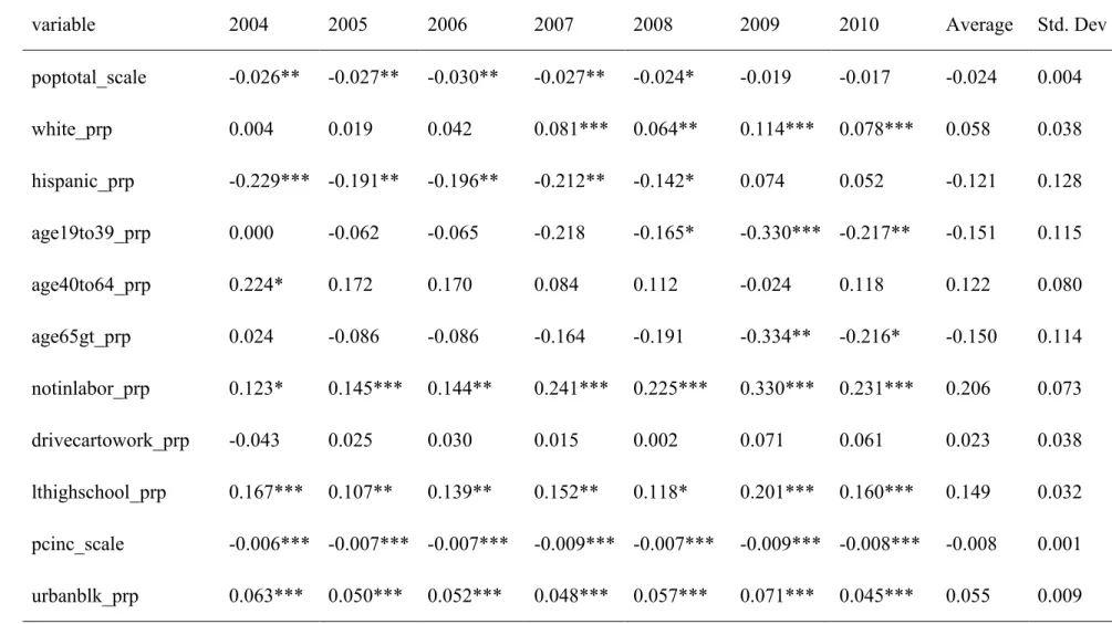
38
standard deviation of the coefficients for each variable. This was compared with the panel logistic model. The individual marginal effects of the logistic model and mean coefficient values are presented in Table 7. We can see that four variables are significant across 7 years; they are the proportion of people not in labor force, people with less than high school education, proportion of urban blocks and per capita income. When the average marginal effects of these variables compared with the ones in random effects model, they have consistent positive or negative sign, but the values in the random effects are smaller than in the year by year analysis. There are obvious relationship between year by year logistic regression and the panel logistic regression.
39
Table 5. Random Effects Linear Regression for All, Urban, and Rural Block Groups
Variables All Block Groups Urban Block Groups Rural Block Groups
N=2133, T=7 N=360, T=7 N=1600, T=7 poptotal_scale -0.465*** 0.045 -0.610*** (0.130) (0.028) (0.184) white_prp 5.575*** -0.193 7.752*** (0.441) (0.121) (0.600) hispanic_prp -7.635*** -0.618** -8.462*** (1.500) (0.271) (2.076) age19to39_prp -5.138*** -0.554* -9.411*** (1.636) (0.325) (2.507) age40to64_prp 6.678*** -0.766 5.768** (1.864) (0.577) (2.617) age65gt_prp -11.260*** -0.932* -16.253*** (1.778) (0.510) (2.552) notinlabor_prp 4.864*** 0.152 7.774*** (1.144) (0.250) (1.587) drivecartowork_prp -0.303 0.395 0.356 (1.318) (0.245) (1.768) lthighschool_prp 7.448*** -0.290* 9.482***
40 (0.971) (0.166) (1.336) pcinc_scale -0.083*** 0.001 -0.129*** (0.019) (0.003) (0.032) urbanblk_prp -1.395*** (0.254) Regional Indicator eastar -2.123*** -0.171** -1.949*** (0.327) (0.068) (0.372) centralar -1.360*** -0.029 -1.369*** (0.343) (0.057) (0.425) nwar -0.830** 0.045 -0.376 (0.338) (0.065) (0.399) sear -0.925** -0.288*** -0.462 (0.365) (0.068) (0.436) swar, 0.048* -0.126** 0.935 (0.357) (0.069) (0.421) wcar -1.571*** -1.267*** (0.347) (0.385) westar -2.507*** -2.601*** (0.376) (0.474)
41
Table 6. Marginal Effects of Random Effects Logistic Regression
Variables All Block Groups Urban Block Groups Rural Block Groups
N=2135, T=7 N=360, T=7 N=1601, T=7 poptotal_scale -0.008** 0.000 -0.009** (0.003) (0.010) (0.004) white_prp 0.016** -0.078* 0.042** (0.007) (0.044) (0.016) hispanic_prp -0.012 -0.153 0.024 (0.021) (0.117) (0.016) age19to39_prp -0.048* 0.080 -0.150** (0.028) (0.089) (0.065) age40to64_prp 0.021 0.027 -0.049 (0.025) (0.097) (0.035) age65gt_prp -0.026 -0.073 -0.098** (0.036) (0.115) (0.046) notinlabor_prp 0.068** 0.087 0.080** (0.028) (0.071) (0.037) drivecartowork_prp 0.001 0.049 0.037 (0.014) (0.065) (0.025) lthighschool_prp 0.071*** 0.006 0.075**
42 (0.023) (0.045) (0.032) pcinc_scale -0.002*** -0.004 -0.002** (0.001) (0.002) (0.001) urbanblk_prp 0.021*** (0.007) Regional Indicator eastar -0.011*** -0.027* -0.009** (0.004) (0.015) (0.004) centralar 0.001 0.001 -0.003 (0.005) (0.018) (0.003) nwar 0.001 -0.007 0.003 (0.005) (0.015) (0.005) sear -0.008** -0.032 -0.001 (0.004) (0.021) (0.004) swar -0.004 -0.012 0.005 (0.005) (0.013) (0.007) wcar -0.008*** -0.004 (0.003) (0.002) westar -0.012*** -0.006** (0.004) (0.002)
Table 7. Logistic Regression Year by Year for All Block Groups (N=2135)
variable 2004 2005 2006 2007 2008 2009 2010 Average Std. Dev
poptotal_scale -0.026** -0.027** -0.030** -0.027** -0.024* -0.019 -0.017 -0.024 0.004 white_prp 0.004 0.019 0.042 0.081*** 0.064** 0.114*** 0.078*** 0.058 0.038 hispanic_prp -0.229*** -0.191** -0.196** -0.212** -0.142* 0.074 0.052 -0.121 0.128 age19to39_prp 0.000 -0.062 -0.065 -0.218 -0.165* -0.330*** -0.217** -0.151 0.115 age40to64_prp 0.224* 0.172 0.170 0.084 0.112 -0.024 0.118 0.122 0.080 age65gt_prp 0.024 -0.086 -0.086 -0.164 -0.191 -0.334** -0.216* -0.150 0.114 notinlabor_prp 0.123* 0.145*** 0.144** 0.241*** 0.225*** 0.330*** 0.231*** 0.206 0.073 drivecartowork_prp -0.043 0.025 0.030 0.015 0.002 0.071 0.061 0.023 0.038 lthighschool_prp 0.167*** 0.107** 0.139** 0.152** 0.118* 0.201*** 0.160*** 0.149 0.032 pcinc_scale -0.006*** -0.007*** -0.007*** -0.009*** -0.007*** -0.009*** -0.008*** -0.008 0.001 urbanblk_prp 0.063*** 0.050*** 0.052*** 0.048*** 0.057*** 0.071*** 0.045*** 0.055 0.009 43
Regional Indicator eastar -0.052*** -0.043*** -0.024* -0.038*** -0.025* -0.041*** -0.016 -0.034 0.013 centralar -0.006 -0.010 0.015 0.003 -0.004 0.014 0.017 0.004 0.011 nwar 0.010 0.012 0.029 0.000 -0.007 -0.018 0.009 0.005 0.015 sear -0.047*** -0.038*** -0.026** -0.004 -0.027* -0.035** -0.006 -0.026 0.016 swar -0.037*** -0.029** -0.019 -0.017 -0.015 -0.009 0.013 -0.016 0.016 wcar -0.035*** -0.027** -0.018*** -0.040*** -0.050*** -0.032** -0.024 -0.032 0.011 westar -0.047*** -0.044*** -0.039 -0.038*** -0.043*** -0.053*** -0.030** -0.042 0.007
Note: *, **, *** denote the marginal effect is significant at 10%, 5% and 1% level.
45 DISCUSSION AND CONCLUSION
In summary, this study separately identified food deserts for both rural and urban areas in Arkansas. The criteria for identifying low access blocks made use of the 1 mile and 10 mile thresholds for both urban and rural blocks. In this research, the data regarding food stores cover 7 years from 2004 to 2010 and the study’s food desert definition follows USDA-ERS approach by considering both distance to food store and income level. Then the association between food deserts and the respective socio-demographic factors driving the food desert likelihood was examined.
The regression and logistic random effects models both yielded similar results. For example block groups with higher unemployment, lower income and lower educational attainment tend to have increasing effects on the distance to the nearest food store. Also these block groups tend to have a higher probability of being food deserts. Thus, food deserts are more likely to exist in areas where there is high prevalence of social and economic deprivation. However, in separate analysis for urban and rural block groups, the urban analysis did not have many significant variables. Results of rural analysis and the overall model are very similar. Compared to past research, similar finding was found with Sharkey and Horel (2008) in minority composition. In their study, they found that minority neighborhood has increasing distance to food store. This research also found that the proportion of Hispanic people in a block group increases; the distance to the nearest food store also decreases. Different finding in the social deprivation part, they found that neighborhood with deprived socioeconomic status have better access to supermarkets. But this study found that block groups with less income,
46
less education, higher people not in labor force tend to have longer distance to the nearest food store. This finding is similar to Algert, Agrawal, and Lewis (2006) study. In Morland and Filomena (2007) paper, they found that White people area has more supermarkets. But in our study, the proportion of while people increases will also increases the distance to food store.
The bordering block groups were also considered in this research, it was thought that people in the bordering areas, especially those close to bordering big cities might go across the state border to do grocery. However, according to Jiao (2002) study, she found out that there are only two relatively big city bordering Arkansas, one is Memphis in Tennessee and the other is Texarkana in Texas. After plotting a radius of 10 mile of the store in these two cities, bordering block groups in Arkansas was out of the radius. Plus there is Mississippi River along the east border. It is very little chance that people in the bordering areas would travel to other States to do grocery.
The contribution of this paper examined the food deserts separately for rural, urban and all block groups within a whole state of Arkansas. Past research usually studied a specific area or city. If a whole state was studied, they did not separate urban and rural areas. In addition, it also evaluated the association of the food deserts with the corresponding block group demographic and socio-economic factors. Some previous studies examined the association of food store environment with their neighborhood factors but did not identified food deserts. Others identified food deserts using different methods but did not consider their community environment.
47
variables because the variable values are based on the 2000 Census data. If for example, time variant variables such as income and population can be collected, the panel regression and logistic models may produce more interesting results. Thus, future studies should devote more time in collecting time varying socio-demographic factors. Other researchers may try to combine the 2010 Census data, but another issue rising here is that 2010 Census has different definition and criteria to classify geographical units, such as block, block group. The other source to get varying income information may come from the Current Population Survey (CPS). But the challenge to use CPS is their geographical level for the report. It provides reliable
estimates at the state level and for 12 of the largest metropolitan statistical areas. No information in a more specific geographical area is provided. If researchers study the food deserts for some areas within the largest metropolitan statistical areas, they may use the income information from CPS. Also the study is only focused on the state of Arkansas and as such future researches can incorporate the methodology used in this paper and extend it to other states as well.
48 REFERENCES
Alwitt, L. F., and T. D. Donley. 1997. “Retail Stores in Poor Urban Neighborhoods.” The Journal
of Consumer Affairs 31(1):139-164.
Algert, S. J., A. Agrawal, and D. S. Lewis. 2006. “Disparities in Access to Fresh Produce in Low-Income Neighborhoods in Los Angles.” American Journal of Preventive Medicine
30(5):365-370.
Apparicio, P., M. Cloutier, and R. Shearmur. 2007. “The Case of Montreal’s Missing Food Deserts: Evaluation of Accessibility to Food Supermarkets.” International Journal of Health Geographics 6(4).
Baker, E. A., M. Schootman, E. Barnidge, and C. Kelly. 2006. “The Role of Race and Poverty in Access to Foods That Enable Individuals to Adhere to Dietary Guidelines.” Preventing
Chronic Disease: Public Health Research, Practice, and Policy 3(3).
Baum, C. F. 2006. An Introduction to Modern Econometrics using Stata. College Station, TX: Stata Press.
Berg, N., and J. Murdoch. 2008. “Access to Grocery Stores in Dallas.” International Journal of
Behavioral and Healthcare Research 1(1): 22-37.
Blanchard, T., and T. Lyson. 2006. “Access to Low Cost Groceries in Nonmetropolitan Counties: Large Retailer and the Creation of Food Deserts.” Working paper, Mississippi State
University, Cornell University.
Block, J. P., R. A. Scribner, and K. B. Desalvo. 2004. “Fast Food, Race/ Ethnicity, and Income: A Geographic Analysis.” American Journal of Preventive Medicine 27(3):221-217.
Clarke, G., H. Eyre, and C. Guy. 2002. “Deriving Indicators of Access to Food Retail Provision in British Cities: Studies of Cardiff, Leeds, and Bradford.” Urban Studies 39(11):2041-2060. Cummins, S., S. Macintyre. 2002. “Food Deserts—Evidence and Assumption in Health Policy
Making.” BMJ 235: 436-438.
---. 1999. “The location of Food Stores in Urban Areas: A Case Study in Glasgow.” British Food
Journal 101(7): 545-553.
Furey S., C. Strugnell, and H. McIlveen. 2001. “An Investigation of the Potential Existence of ‘Food Deserts’ In Rural And Urban Areas of Northern Ireland.” Agriculture and Human Values 18: 447-457.
Guy, C., G. Clarke, and H. Eyre. 2004. “Food Retail Change and the Growth of Food Deserts: A Case Study of Cardiff.” International Journal of Retail and Distribution Management
49
Hendrickson, D., C. Smith, and N. Eikenberry. 2006. “Fruit and Vegetable Access in Four Low-Income Food Deserts Communities in Minnesota.” Agriculture and Human Values
23:371-383.
Jiao, Y. 2012. “Food Environment and Child Obesity.” MS thesis, University of Arkansas. Kaufman, P. R. 1999. “Rural Poor Have Less Access to Supermarkets, Large Grocery Stores.”
Rural Development Perspectives 13(3):19-26.
Larsen, K., and J. Gilliland. 2008. “Mapping the Evolution of Food Deserts in A Canadian City: Supermarket Accessibility in London, Ontario, 1961-2005.” International Journal ofHealth
Geographics 7(16).
McEntee, J., and J. Agyeman. 2010. “Towards the Development of a GIS Method for Identifying Rural Food Deserts: Geographic Access in Vermont, USA.” Applied Geography 30:
165-176.
Morland, K., S. Wing, A. D. Roux, and C. Poole. 2002. “Neighborhood Characteristics
Associated with the Location of Food Stores and Food Service Places.” American Journal of
Preventive Medicine 22(1): 23-29.
Morland, K., and S. Filomena. 2007. “Disparities in the Availability of Fruits and Vegetables Between Racially Segregated Urban Neighborhoods.” Public Health Nutrition 10(12): 1481–1489.
Morton L. W., and T. C. Blanchard. 2007. “Starved for Access: Life in Rural America's Food Deserts.” Rural Realities 1(4):1-10.
Powell, L.M., F. J. Chaloupka, and Y. Bao. 2007. “The Availability of Fast-Food and Full-Service Restaurants in the United States, Associations and Neighborhood Characteristics.” American Journal of Preventive Medicine 33(4s): s240-s245.
Sharkey, J. R., and S. Horel. 2008. “Neighborhood Socioeconomic Deprivation and Minority Composition Are Associated with Better Potential Spatial Access to the Ground-Truthed Food Environment in a Large Rural Area.” The Journal of Nutrition 138(3): 620-627. Short, A., J. Guthman, and S. Raskin.2007. “Food Deserts, Oases, or Mirages? Small Markets
and Community Food Security in the San Francisco Bay Area.” Journal of Planning
Education and Research 26: 352-364.
Smoyer-Tomic, K. E., J. C. Spence, and C. Amrhein. 2006. “Food Deserts in the Prairies?
Supermarket Accessibility and Neighborhood need in Edmonton, Canada.” The Professional
Geographer 58(3):307-326.
50
Measurement of Food Access in Portland, Oregon.” Paper presented at National Poverty Center/USDA Economic Research Service research conference, Washington DC, 23rd January.
U.S. Department of Agriculture, Economic Research Service. 2009. Access to Affordable and Nutritious Food: Measuring and Understanding Food Deserts and Their Consequences.
Washington DC, June.
Wrigley, N. 2002. “Food Deserts in British Cities: Policy Context and Research Priorities. Urban
Studies, 39(11): 2029-2040.
Zenk, S. N., A. J. Schulz, B. A. Israel, S. A. James, S. Bao, and M. L. Wilson. 2005.
“Neighborhood Racial Composition, Neighborhood Poverty, and the Spatial Accessibility of Supermarkets in Metropolitan Detroit.” American Journal of Public Health 95(4): 660-667.