UNIVERSIDAD AUT ´
ONOMA DE MADRID
ESCUELA POLIT´
ECNICA SUPERIOR
TRABAJO FIN DE M ´ASTER
Support Vector Machines and Multi-Task Learning
M´aster Universitario en Investigaci´on e Innovaci´on en TIC
Autor: Carlos Ruiz Pastor
Tutor: Jos´
e R. Dorronsoro Ibero
Cotutor: Carlos M. Ala´ız Gud´ın
Departamento de Ingenier´ıa Inform´aticaContents
Contents ii
List of Figures v
List of Tables vi
List of Algorithms viii
1 Introduction 1
1.1 Motivation . . . 1
1.2 Objectives . . . 1
1.3 Structure . . . 2
2 Support Vector Machines 3 2.1 Kernel-Induced Feature Spaces . . . 3
2.2 Optimization Theory . . . 6
2.2.1 Problem Formulation . . . 6
2.2.2 Lagrangian Theory . . . 7
2.3 Support Vector Machines . . . 11
2.3.1 Motivation . . . 11
2.3.2 Analysis . . . 15
2.3.3 Kernel Trick . . . 18
2.4 SMO Algorithm . . . 20
2.4.1 Update Step . . . 20
2.4.2 Selection Step: Selecting the Optimal (U, L) . . . 23
2.4.3 Computational Cost . . . 26
3 Multitask Learning 29 3.1 Linear Support Vector Machines for Multitask Learning . . . 29
3.1.1 Analysis . . . 30
3.1.2 Formulation as a Single-Task Problem . . . 33
3.2 Multiple Kernel Support Vector Machines for Multitask Learning . . . 36
3.3 GSMO Algorithm . . . 39
3.3.1 Update Step . . . 39
3.3.2 Selection Step . . . 43
3.3.3 Computational Cost . . . 46
3.4 Single Bias Multi-task SVM . . . 47 iii
4 Experiments 49
4.1 Implementation Details . . . 49
4.1.1 LIBSVMand Scikit-learn . . . 49
4.1.2 The mtlSVMClass . . . 51
4.2 A first application: Prediction of school grades . . . 51
4.2.1 Dataset Description . . . 52
4.2.2 Results . . . 53
4.3 Energy Forecasting . . . 56
5 Discussion and Further Work 61
List of Figures
2.3.1 Distance between a point and a plane . . . 12
2.3.2 Slack variables for SVC . . . 13
2.3.3 SVR error function . . . 14
2.3.4 Regressor plane and tube of SVR . . . 15
2.3.5 Illustration of support vectors . . . 19
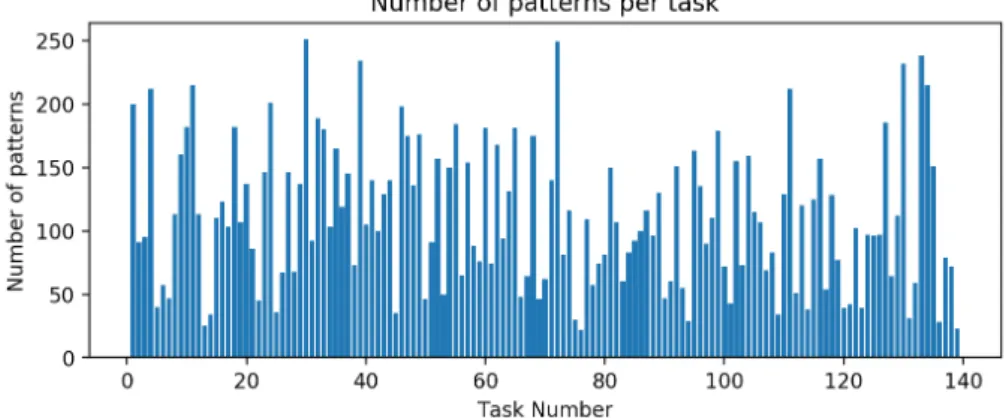
4.2.1 Number of patterns per task . . . 53
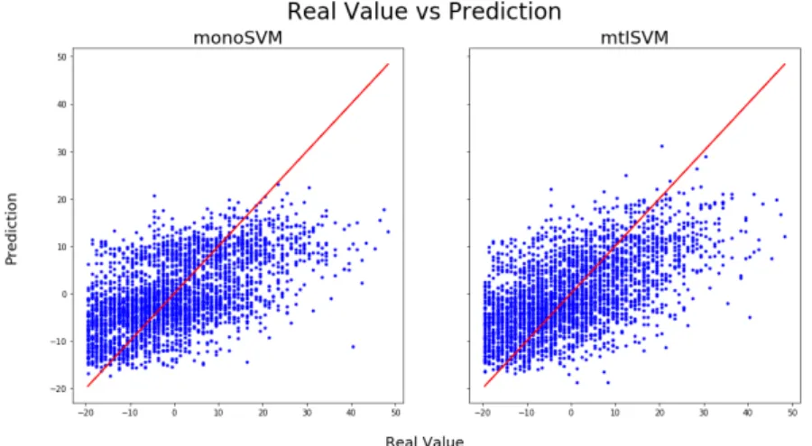
4.2.2 Real value and Prediction . . . 54
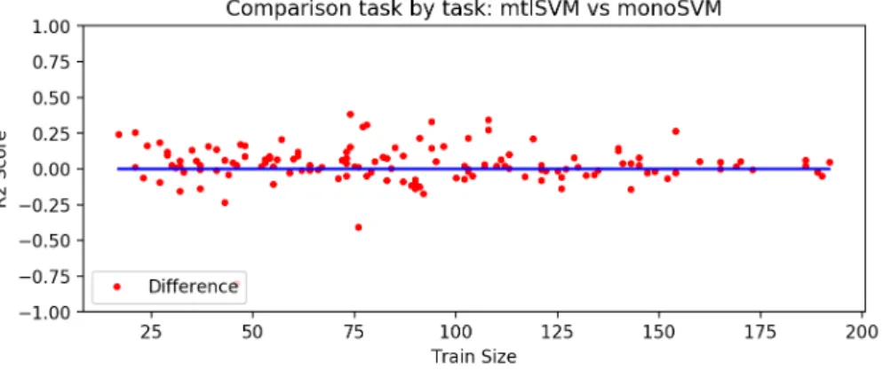
4.2.3 R2 score per task . . . 55
4.2.4 MAE score per task . . . 55
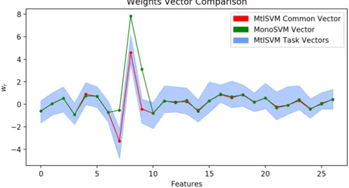
4.2.5 Weights Vectors Comparison . . . 56
4.3.1 Solar production by hour . . . 58
4.3.2 Solar Prediction against Production in all models . . . 59
List of Tables
2.3.1 Classification ofSupport Vectors in terms of the value of αi. . . 18
4.3.1 Optimal parameters for the models considered. . . 59 4.3.2 MAE of each model in Majorca, Tenerife and in average. . . 59
List of Algorithms
1 SMO . . . 27 2 GSMO . . . 47
Resumen
En la mayor´ıa de casos los problemas que se resuelven utilizando aprendizaje autom´atico no est´an aislados, sino que hay numerosas tareas similares con las que est´an relacionados. El aprendizaje multitarea es una aproximaci´on del aprendizaje autom´atico que trata de resolver m´ultiples tareas al mismo tiempo, logrando as´ı una perspectiva m´as amplia del problema global. Las m´aquinas de vectores soporte son unos de los m´etodos m´as populares en aprendizaje autom´atico, y han demostrado ser modelos ´utiles que adem´as est´an apoyados por la teor´ıa de optimizaci´on convexa.
En este trabajo estudiamos la adaptaci´on de las m´aquinas de vectores soporte con el objetivo de encajar en un entorno multitarea. Nuestro primer paso para lograr esto es ex-plorar la teor´ıa de optimizaci´on convexa, espec´ıficamente las m´aquinas de vectores soporte. Hacemos un resumen de los problemas de optimizaci´on, incluyendo las condiciones KKT, as´ı como el truco del kernel y el algoritmo SMO, que es el m´as popular para entrenar SVMs. Basamos nuestro estudio en dos adaptaciones previas de las SVMs al aprendizaje multitarea, desarrollando sus ideas y presentando las similitudes y diferencias entre am-bas aproximaciones. Tambi´en analizamos la relaci´on entre los enfoques para obtener las ventajas que cada uno ofrece.
Para probar la precisi´on de las SVMs multitarea proponemos dos experimentos uti-lizando datos reales. El primero utiliza datos de estudiantes de institutos de Inglaterra y el objetivo es predecir los resultados de los estudiantes en un test espec´ıfico. En estos experimento se utilizan datos de estudiantes de 139 institutos, y la predicci´on de las notas en cada instituto se observa como una tarea distinta. El segundo experimento consiste en predecir la producci´on solar, medida como un porcentaje, en dos islas de Espa˜na: Mallorca y Tenerife. Aunque ambas islas pertenecen a Espa˜na la distancia entre ellas es de m´as de 2.200 km. Esto hace que las predicciones en cada isla sean tareas separadas. En estos ex-perimentos comparamos el enfoque multitarea con un enfoque global monotarea y, cuando es posible, entrenando un modelo distinto para cada tarea.
A partir de los resultados obtenidos podemos observar que el enfoque multitarea obtiene mejores resultados que el enfoque global monotarea. En el caso de los datos de institutos obtenemos un MAE de 8,226 puntos usando el enfoque monotarea y uno de 8,039 puntos con el multitarea. Adem´as, esta mejora tiene lugar no solo globalmente sino tambi´en en la comparaci´on tarea a tarea el enfoque multitarea obtiene mejores resultados en 90 de las 139 tareas. En el experimentos solar obtenemos una mejora de 0.45 % en Tenerife usando el modelo multitarea, mientras que en Mallorca el error es 0.15 % mayor; por tanto, se obtiene globalmente una mejora de 0.15 %. Estos resultados dan la motivaci´on para una investigaci´on futura con el objetivo de desarrollar todo el potencial de las SVMs multitarea.
Abstract
In most cases the problems we solve using machine learning are not isolated; instead there are several similar and related tasks. Multi-task learning is an approach of machine learning that tries to solve multiple related tasks at the same time, achieving a broader perspective of the global problem. Support vector machines are one of the most popular methods in machine learning, and they have proven to be really useful models which are also supported by the convex optimization theory.
In this work we study the adaptation of support vector machines in order to match a multi-task learning framework. Our first step to achieve this goal is to explore convex optimization theory and more specifically, support vector machines theory. We will give an overview of the optimization problems, including the KKT conditions, as well as the kernel trick and the SMO algorithm, the most used algorithm to train SVMs. We base our study in two previous adaptations of SVMs to multi-task learning, developing their ideas and presenting the similarities and differences between the two approaches. We also analyze the relation between the approaches and the possible advantages each one offers.
To test the accuracy of multi-task SVMs we propose two experiments using real data. The first one uses data from English school students and the goal is to predict the results of the students in a specific test. In this experiment, 139 different schools are used and predicting the marks of their students in each one of them is seen as a different task. Our second experiment consists on predicting the solar production measured as a percentage in two different islands of Spain: Majorca and Tenerife. Although both islands are part of Spain, the distance between both is roughly 2,200 km, making the predictions separate tasks. In our experiments we compare the multi-task approach with a single-task global approach and, when possible, with a model specialized for each task.
From the results obtained we can observe that multi-task approach gets better results than a single-task global approach. In the case of the school data we get a MAE of 8.226 points using the single-task approach while the multi-task approach achieves 8.039. Moreover, we see that this improvement takes place not only globally, but in a task by task comparison the multi-task approach performs better in 90 tasks out of 139. In the solar experiment we obtain an improvement of 0.45% in the MAE of the prediction in Tenerife using the multi-task model, while the error in Majorca is 0.15% worse than using a single-task approach, resulting in a global improvement of 0.15%. This results give the motivation to do further research in this area with the goal of finding the full potential of multi-task SVMs.
Acknowledgements
En primer lugar, quiero agradecer a mi tutor, Jos´e R. Dorronsoro, su dedicaci´on y paciencia porque, a pesar de los abundantes compromisos, siempre es capaz de sacar un rato para ayudar o corregir los fallos. Tambi´en agradezco su supervisi´on y ayuda durante todo el a˜no en el que me ha guiado y cuyo resultado es este trabajo, en el que siempre ha puesto en primer lugar mi aprendizaje y formaci´on. Aprecio que, a pesar de su exigencia, ha valorado mi trabajo y me ha dado ´animos para continuar por esta senda.
Agradezco tambi´en a mi cotutor Carlos M. Al´aiz del que destaco su atenci´on en los detalles y sus geniales ideas. Ha sido de gran ayuda tanto mostr´andome los fallos que tengo como ofreciendo soluciones. Tambi´en aprecio su capacidad para entenderme r´apidamente y sus acertadas aportaciones, haciendo que sea realmente f´acil trabajar con ´el.
Agradezco a Sara Dorado su contante apoyo, aprecio el hecho de haberme escuchado cuando ten´ıa dudas y estar siempre para ayudarme. Doy tambi´en las gracias a mi compa˜nero Alejandro Catalina, del que destaco su motivaci´on e inter´es, ya que siempre ofrece una mano de forma altruista.
Doy las gracias a la C´atedra UAM-IIC de Ciencia de Datos y Aprendizaje Autom´atico por la ayuda de m´aster concedida. Por ´ultimo, quiero agradecer a mi familia su apoyo que me permite dedicarme a la investigaci´on sin pedirme nada a cambio.
Chapter 1
Introduction
In this chapter we will first present the motivation behind this work, which is mainly to study the adaptation of the SVM’s theory to a multi-task learning framework. We will also define the objectives we aim to achieve to do this. Finally, we will describe the structure followed in this work.
1.1
Motivation
Multi-task learning is a field inside the transfer learning theory, where the goal is to combine knowledge from different models in order to have a larger quantity of information to learn from. In particular, multi-task learning aims to combine different datasets from problems that are related, which receive the name of tasks; then, all tasks are solved at the same time and the solution of each single one makes use of the knowledge of the remaining tasks. That way, the amount of information that we can use is not constrained to the data we have collected for any specific problem; instead, we can take advantage of data collected for similar problems. This is especially useful in those cases where the amount of data avalaible is not enough to train a single operative model for each task, but the combination of multiple datasets is sufficient. On the other side, Support Vector Machines (SVMs) are popular models in machine learning due to its multiple characteristics and the theory that supports them. Our main motivation for this work is to study the adaptation SVMs in order to use them in a multi-task learning framework.
1.2
Objectives
The objective of this work is two-fold: in first place, based on previous works [1, 2], we want to connect the different approaches that have been made and to formalize the multi-task SVM. In the second place, we put our focus on the comparison of the multi-task SVR and traditional single-task SVRs. For our first goal, we will study the ideas presented in [1] and the posterior approach of [2] and we show its similarities and differences. Although at first glance both works are not connected we will see that the second one can be formulated as a generalization of the first one. For the second goal, we will carry out experiments using two different datasets. In the first place, we will work with a dataset containing data from high schools of England that has been traditionally used for multi-task purposes [3, 1, 4]. In the second place, we will use a multi-task dataset, in which we combine the solar production of the islands of Majorca and Tenerife in Spain, interpreting each island’s solar production forecast as a separate task. In order to carry out these experiments the implementation of an SVR of Scikit-learnwill be used. However, in order to make an easy implementation
of the multi-task SVR a hybrid approach between those of [1] and [2] will be developed and used.
1.3
Structure
This work is structured as follows: in Chapter 2 we will cover the mathematical fundamen-tals of SVR, mainly, the kernel induced feature spaces in Section 2.1 and the optimization theory in Section 2.2; in Section 2.3 we will also develop the theory of the traditional single-task SVM; finally we will present the SMO algorithm in Section 2.4, an algorithm used to train SVMs. In Chapter 3 we will develop the theory of the multi-task SVRs. In the first place, in Section 3.1 we will present the approach made in [1], which is called Regularized Multi-Task Learning, where the kernel used is linear and the bias is omitted. In Section 3.2 we will develop the ideas of [2] and we will show the connection with Regularized Multi-Task Learning as well. We will also present the algorithm needed to train the multi-task SVR that receives the name of Generalized SMO. In Chapter 4 we present the experiments carried out and their results. First, in Section 4.1 we explain the implementation used for the experiments; after this, Section 4.2 contains the results of the experiment that use the school dataset, whereas in Section 4.3 we present the experiment carried out using the solar production datasets. Finally, in Chapter 5 we will discuss the results obtained and we will present the ideas that are left for further work.
Chapter 2
Support Vector Machines
This chapter has the purpose of covering the theory necessary for the rest of this work. In first place it gives an overview of the kernel-induced feature spaces and optimization theory in Section 2.1 and Section 2.2 respectively; both topics are very important because they lie underneath the theory of Support Vector Machines. Support Vector Machines (SVMs) are explained in the third section of this chapter as they are presented as an application of the general convex theory covered previously. We will also see the motivation that makes SVMs interesting models in a machine learning framework, as well as the algorithm SMO, which is the most popular one for training these models. It is important to remark that this chapter has its focus on single-task classical SVMs and does not cover multi-task SVMs, which will be explained in Chapter 3.
2.1
Kernel-Induced Feature Spaces
In machine learning, specifically in supervised classification or regression, each patternx, a point of a feature space X which is usually a subspace of Rd, is assigned a label or target; our goal is to learn the underlying relations in order to assign labels or targets to new examples. To do this several hypotheses can be chosen, and among all, linear hypotheses are the simplest and the easiest to explain. Linear models have multiple advantages such as explainability and often explicit solutions of the problem. Because of this they are one of the most popular examples of machine learning algorithms and historically the first to appear; see for example linear regression or Rosenblatt’s perceptron [5] algorithms, which are linear algorithms for regression and classification respectively. Nevertheless, linear models are very limited and usually they are not expressive enough for real-world applications. Real-world data include complex relations that may not be linear and thus it is necessary a model that is capable of detecting those non-linear relations. One possible solution for introducing non-linearity to models is to map the original points on X to a large dimensional space F through some mapping functionφ, that is
φ:X ⊂Rd→ F ⊂RD
x= (x1, . . . , xd)t7→φ(x) = (φ(x)1, . . . , φ(x)D)t,
where D can be even infinite resulting then in an infinite dimensional space F. At this point it is relevant to recall one important property that is usually present in linear models, that is the possibility of writing the models in terms of the Gramm matrix G. The matrix
G is constructed using the inner products of the patterns. Given a data matrix X where each row is the transpose of a pattern xi ∈ X of our sample of size N, then the Gramm
matrix is G= hx1, x1i hx1, x2i . . . hx1, xNi hx2, x1i hx2, x2i . . . hx2, xNi .. . ... . .. ... hxN, x1i hxN, x2i . . . hxN, xNi .
This means that we expect that the model is no longer dependent on the data itself but on the inner products of the patterns. This property paves the way for the introduction of kernel functions and kernel-induced features.
The problem of mapping the data on a larger space is its computational cost, that is linearly dependent onD, the dimension of the new spaceF. This is where kernel functions play an important role.
Definition 2.1.1. A kernel function k is a function such that for all points x, z in our original feature space X verifies
k(x, z) =hφ(x), φ(z)i,
where φis a mapping from the original space to a new feature space F induced by k.
If for a mapping functionφwe know its corresponding kernel functionk, then we have a direct way of computing the Gramm matrix on the new space F and moreover, it is no longer dependent on φ. For example, in the original space the kernel is
k(x, z) =hx, zi,
this is called a linear kernel, and φ(x) =x. Another example is the polynomial kernel:
k(x, z) = (hx, zi+c)2= d X i=1 xizi+c ! d X j=1 xjzj +c = d X i=1 d X j=1 xixjzizj+ 2c d X i=1 xizi+c2.
From this definition it is easy to see that the transformation whose inner product is this polynomial kernel is the following
φ(x) = x1x1, x1x2, . . . , x1xd, . . . , xdx1, . . . , xdxd, √ 2cx1, . . . , √ 2cxd, c ,
where the dimension D isd2+d+ 1.
Although the use of a kernel functionkis attractive, it seems that using this approach requires finding a complicated feature space and then work out the inner product until finding the functionkin terms of the original features, which is not practical and definitely not trivial. However, in practice the approach is taken reversely: the kernel function is de-fined directly and hence the feature space is implicitly dede-fined, which is much easier to work with. Nevertheless, to do this, it is necessary to know what are the properties that ensure that k(x, z) is a kernel function for some appropiate feature space. The characterization of a kernel function is given by Mercer’s Theorem [6].
Theorem 2.1.1 (Mercer’s Theorem). Let X ⊂Rd and suppose that k(x, z) :R×R7→R
is a continuous symmetric function such that the integral operator Tk:L2(X) → L2(X)
associated to k and defined as
f(x)7→(Tkf)(x) =
Z
X
2.1. Kernel-Induced Feature Spaces 5
is non-negative, which means Z
X ×X
k(x, z)f(x)f(z)dxdz≥0,∀f ∈L2(X). (2.1.1)
Then we can expand k(x, z) in a uniformly convergent series (onX × X) in terms of Tk’s orthonormal eigen-functions φj ∈ L2(X) and non-negative associated eigenvalues λj ≥0
as k(x, z) = ∞ X l=1 λlφl(x)φl(z).
The complete proof of Mercer’s Theorem is out of the scope of this work. However, we can have an intuition. Note in first place that the operator Tk is self-adjoint, we can see it in the following way:
hTkf, gi= Z X (Tkf)(x)g(x)dx= Z X Z X k(x, z)f(z)dz g(x)dx = Z X Z X k(z, x)f(z)dz g(x)dx= Z X Z X k(z, x)g(x)f(z)dzdx = Z X f(z) Z X k(z, x)g(x)dx dz=hf, Tkgi.
Moreover, it can be proven thatTk is a compact operator; hence; we can apply the Spectral
Theorem for compact operators on Hilbert Spaces [7, Volume 1, Chapter 8]:
Theorem 2.1.2 (Spectral Theorem). Suppose T is a compact self-adjoint operator on a Hilbert space F. Then there is an orthonormal basis of F consisting of eigenvectors
φi(x)∈L2(X) of T real eigenvalues λi such that
λiφi(x) = (T φi)(x).
Furthermore, it can be seen that
∞ X i=1 λikφi(x)φi(z)k<∞, and therefore, ∞ X i=1
λiφi(x)φi(z)
is uniformly convergent and it can be proved that it converges to k(x, z). With the result of Mercer’s Theorem, the feature space F is span{φ(x) :x∈ X } and the feature map φ
from the original space X to the new feature spaceF is automatically given by
φ(x) =pλ1φ1(x), p λ2φ2(x), . . . , p λkφk(x), . . . .
Moreover, a more practical characterization of a kernel can be given with the following definition of kernel function also given by Mercer.
Definition 2.1.2 (Kernel Function Characterization). Given a non-empty space X we say that a symmetric function k(x, y) : X × X 7→ R is a kernel if for any finite sample
x1, . . . , xn∈ X the matrix
K = (k(xi, xj))i,j , i= 1, . . . , n, j= 1, . . . , n
2.2
Optimization Theory
2.2.1 Problem Formulation
Most problems in machine learning aim to find an element that maximizes or minimizes some functional. In the case of linear models this is finding a vector w that minimizes an objective function, often restricted to some constraints. The optimization theory has the goal of characterizing such solutions, and moreover, to develop algorithms to find them efficiently. An important example of this is the duality theory developed for linear models, which gives easy-to-check characterization rules for a solution of the problem. It is particularly interesting the case of convex optimization due to the inherent properties of convexity. The general problem is to find the solution w∗ in a set Ω that minimizes some objective function given some constraints.
Definition 2.2.1 (Primal Problem). Given the functions f, gi, hj, i ∈ {1, . . . , k}, j ∈ {1, . . . , m} defined in Ω∈Rd7→R , the primal optimization problem is defined as
min
w∈Ωf(w)
s.t. gi(w)≤0, i∈ {1, . . . , k}, hj(w) = 0, j∈ {1, . . . , m}.
where f(w) is the objective function and gi, hi are the inequality and equality constraints,
respectively.
For the sake of simplicity we will use the following notation • g(w)≤0 instead of gi(w)≤0, i∈ {1, . . . , k}.
• h(w) = 0 instead of hj(w) = 0, j ∈ {1, . . . , m}.
The region of the space where all the constraints are satisfied is called the feasible region. Definition 2.2.2 (Feasible Region). The feasible region is the region of the domain of
f(w) where all the restrictions are fulfilled. That is,
R={w∈Ω :g(w)≤0, h(w) = 0} .
Given the definition of feasible region, we can state the definition of global and local solutions.
Definition 2.2.3 (Global and local solution). We say that w∗ ∈ R is a global solution
of the optimization problem if f(w∗)≤f(w)∀w ∈ R. Moreover, we can say that w∗ is a
local solution if ∃such that f(w∗)≤f(w)∀w∈ R,kw−w∗k< .
Any solutionw∗ must fulfill the equality and inequality conditions; an inequality con-dition gi(w) is said to be active ifg(w∗) = 0 and inactiveif g(w∗) <0. While equality
constraints are always active, this is not the case for inequality constraints. In order to transform a constraint from an inequality to an equality, slack variables ξi are added. In that way, the restriction gi(w) ≤0 is transformed to gi(w) +ξi = 0, ξi ≥0. These slack
variables indicate the looseness of the constraint gi in a particular solution; therefore, an
active constraint will haveξi= 0. Moreover, an interesting result that we will prove below is that a convex function ensures that any local minimum is a global one; therefore sim-plifying the task of finding the global minimum. This property, although very likeable, is not fulfilled in general, which is the reason why the optimization theory is closely related to convexity; thus it is important to recall some definitions concerning convexity.
2.2. Optimization Theory 7
Definition 2.2.4 (Convex Set). A setΩ is said to be convex if and only if ∀u, v∈Ω and
λ∈(0,1)
λu+ (1−λ)v∈Ω. (2.2.1)
Notice that the intersection of two convex sets is also convex. Given this definition is immediate to define a convex function.
Definition 2.2.5 (Convex Function). A function f :X ⊂Rd7→ Ris convex if and only
if its epigraph, that is n
(x, t)∈Rd+1, x∈Rd, t≥f(x)o ,
is a convex set. Equivalently, f is convex if and only if ∀x, y∈ X and λ∈(0,1)
f(λx+ (1−λ)y)≤λf(x) + (1−λ)f(y). (2.2.2)
Now, it is easy to see that local minimum of a convex function implies global minimum. Proposition 2.2.1. Any local minimum w∗ of a convex function f(w) is also a global minimum of f(w).
Proof. Let w∗ ∈ Ω be a local minimum, then f(w∗) ≤ f(λu+ (1−λ)w∗) ∀u ∈ Ω for a small enough λ >0. Since f is convex we can write the following
f(w∗)≤f(λu+ (1−λ)w∗)≤λf(u) + (1−λ)f(w∗),
which implies
f(w∗)≤f(u),∀u∈Ω.
Any optimization problem in which the set Ω, the objective function f and all the constraints are convex is said to be a convex problem. It is easy to see that the feasible region of a convex problem is convex since it is the intersection of the set Ω with the epigraphs of the constraints functions, which are convex. Since our goal is to work with SVMs, we will restrict ourselves to a simpler case where all the restrictions are linear.
2.2.2 Lagrangian Theory
The Lagrangian theory, developed firstly by Fermat and then generalized by Lagrange, aims to characterize the solutions of the optimization problems. In order to get a better understanding we will start with the simplest case, where there are no constraints. In this case the Fermat Theorem [8] applies.
Theorem 2.2.1 (Fermat’s Theorem). A necessary condition for w∗ to minimize f(w) ∈
C1, is ∇wf(w∗) = 0. If we assume f(w) a convex function, then ∇wf(w∗) = 0 is a
necessary and sufficient condition for w∗ to minimize f.
It is well known that a pointw∗ where∇wf = 0 is a critical point, and, if the function is convex it must be a global minimum. However, when some restrictions are imposed, the condition ∇wf = 0 might not be achieved in the feasible region. To solve this we can
notice some aspects of the problem that can help us to have a better intuition. We want to advance in the opposite direction of the one indicated by the gradient ∇wf. However, since the constraints have to be met, this may not be done freely. Let us restrict ourselves first to equality constraints hj(w) = 0, which can be seen as the zero-level curve of hj(w);
therefore, hj(w) = 0 is a curve such that its tangent vector is perpendicular to ∇hj(w) at every point in it. If a point is in the feasible region and we want to move to another point, we have to do it perpendicularly to∇hj(w). This means that, intuitively, in order to
minimizef(w) we have to move in the component of the gradient∇wfthat is perpendicular
to∇hj. When there are multiple constraints we have to move perpendicularly to
H= span{∇hj(w), j∈ {1, . . . , m}}.
This can be done only if ∇wf(w) ∈ H/ ; hence, we can express this condition in a simple way: w∗ is a solution of the problem with constraints if∃β1, . . . , βm such that
∇wf(w∗) =
m
X
j=1
βj∇hj(w∗) ; (2.2.3)
thus, given a problem with objective function f and equality constraints hj we can define its Lagrangian as L(w, β) =f(w) + m X j=1 βjhj(w).
Given this definition and the previous results it is easy to prove the following theorem [8, Chapter 5, Theorem 5.8].
Theorem 2.2.2 (Lagrange). Necessary conditions of w∗ for being a solution of a problem with objective function f(w) and equality constraints hj(w) = 0, j∈ {1, . . . , m} are
∇wL(w∗, β∗) = 0,
∇βL(w∗, β∗) = 0,
for some values β∗. These conditions are sufficient iff(w) andhj(w), j∈ {1, . . . , m}, are
convex.
It is clear to see that the first condition is the condition (2.2.3) while the second one ensures the feasibility of w∗.
We now consider the more general case of an optimization problem, with both equality and inequality constraints. Then, we can give the following definition.
Definition 2.2.6 (Lagrangian). Given an optimization problem with objective function
f(w), equality constraints hj(w) = 0, j ∈ {1, . . . , m} and inequality constraints gi(w) ≤ 0, i∈ {1, . . . , k} we define the Lagrangian of such problem as:
L(w, β) =f(w) + k X i=1 αigi(w) + m X j=1 βjhj(w) =f(w) +αg(w) +βh(w),
where α≥0 and β are called the Lagrange multipliers.
From the definition of Lagrangian we can define the Dual Function.
Definition 2.2.7 (Dual Function). Given an optimization problem and its Lagrangian
L(w, α, β) we define its Dual Function as
Θ(α, β) = inf
w∈ΩL(w, α, β). Now we can define the Dual Problem.
2.2. Optimization Theory 9
Definition 2.2.8(Dual Problem). The Dual Problem of a LagrangianL(w, α, β)is defined as:
max
α,β Θ(α, β)
s.t. α≥0,
where Θ(α, β) is the Dual Function.
To connect the primal and dual problem we have the duality theorems. The first one, Weak Duality Theorem [8, Chapter 5, Theorem 5.15], is the following.
Theorem 2.2.3 (Weak Duality Theorem). Let (α, β) and w be feasible solutions (not necessarily optimal) for the dual and primal problems respectively; then
Θ(α, β)≤f(w).
Proof. Using the definition of the dual function and the feasibility ofwand α,
Θ(α, β) = inf w∈ΩL(w, α, β)≤f(w) + k X i=1 αigi(w) + m X j=1 βjhj(w)≤f(w).
This theorem provides two useful corollaries.
Corollary 2.2.1. The optimal value Θ(α∗, β∗) of the dual is upper bounded by the optimal value of the primal f(w∗), that is
Θ(α∗, β∗)≤f(w∗).
Corollary 2.2.2. Any tuple (α∗, β∗) and w∗ such that
Θ(α∗, β∗) =f(w∗)
are optimal solutions for both the dual and the primal problems respectively.
The difference between the optimal values of the primal and the dual is called thedual gap and therefore, having a null dual gap is a sufficient condition (although not necessary in general) to find optimal solutions. This idea motivates the second duality theorem [8, Chapter 5, Theorem 5.20].
Theorem 2.2.4 (Strong Duality Theorem). Given a convex problem
arg min
w∈Ω
f(w)
s.t. gi(w)≤0, i∈ {1, . . . , k}, hj(w) = 0, j ∈ {1, . . . , m},
if gi and hj are affine functions, then the dual gap of the problem is zero.
This theorem has the following consequence: given a solution (α∗, β∗) of the dual problem, we know the minimum value of the primal functionf(w∗) = Θ(α∗, β∗). Moreover, in some particular cases where we have an equation that expresses w in terms of (α, β), we can recover the primal solution w∗ from (α∗, β∗). After this result, we can present the Karesh-Kuhn-Tucker conditions [9] to characterize the optimal solution of an optimization problem.
Theorem 2.2.5 (KKT Theorem). Suppose a convex optimization problem with affine constraints. Then, w∗ is an optimal solution of the primal problem if and only if there exist (α∗, β∗) such that:
∂L(w, α, β) ∂w w∗,α∗,β∗ = 0, ∂L(w, α, β) ∂β w∗,α∗,β∗ = 0, αi∗gi(w∗) = 0, i∈ {1, . . . , k}, gi(w∗)≤0, i∈ {1, . . . , k}, α∗i ≥0, i∈ {1, . . . , k}.
Proof. Since the KKT conditions are necessary and sufficient we will split the proof for both cases. We will first check necessity; ifw∗is an optimal solution of the primal problem, by the Strong Duality Theorem 2.2.4, we know that
Θ(α∗, β∗) =L(w∗, α∗, β∗) =f(w∗), and since Θ(α∗, β∗) = inf w∈ΩL(w, α ∗ , β∗),
w∗ must be a minimum ofL, which is convex onw; therefore, we have
∂L(w, α∗, β∗) ∂w w∗= 0
(first KKT condition). Since w∗ is a solution, it is feasible; therefore
∂L(w∗, α∗, β) ∂β β∗ =h(w ∗) = 0
(second KKT condition), and gi(w∗)≤0, i∈ {1, . . . , k} (fourth KKT condition). Finally, using the Weak Duality Theorem we can write the following,
Θ(α, β)≤ L(w∗, α, β)≤f(w∗),
for everyα, β. However, using the Strong Duality Theorem, it must exist a solution (α∗, β∗) with α∗ ≥0 (last KKT condition) of the dual that fulfills
Θ(α∗, β∗) =L(w∗, α∗, β∗) =f(w∗) ; then, using the second equality we have
f(w∗) + k X i=1 α∗igi(w∗) + m X j=1 βj∗hj(w∗) =f(w∗).
Usinggi(w∗)≤0 and α >0 we have then
αigi = 0, i∈ {1, . . . , k},
which is the third KKT condition.
To prove sufficiency, we need to see thatw∗is an optimal solution of the primal problem. It is therefore sufficient to see Θ(α∗, β∗) =f(w∗). Using the first condition we have
Θ(α∗, β∗) = inf
w∈ΩL(w, α
2.3. Support Vector Machines 11
Using the remaining properties we can write the following L(w∗, α∗, β∗) =f(w∗) + k X i=1 α∗igi(w∗) + m X j=1 β∗jhj(w∗) =f(w∗),
where the first equality is just the definition and the second one uses the second and third KKT conditions.
2.3
Support Vector Machines
We will dedicate this section to the motivation and analysis of Support Vector Machines, which are one of the most popular models in machine learning. Their popularity can be related to their idea of maximum separability and the extensive theory that supports this. The first subsection aims to present the idea that motivates SVMs and their utility. In the second subsection we will perform a more detailed analysis of the properties of SVMs. Finally, the last subsection is devoted to the SMO algorithm, which is currently the most popular method for solving SVMs.
2.3.1 Motivation
Before showing the SVMs motivation, it is necessary to define some concepts. In first place, a binary classification problem is a problem in which we have patterns xi ∈
X ⊂ Rd , i = 1, . . . , N labeled with y
i ∈ Y , i = 1, . . . , N, where |Y| = 2, for example
Y = {−1,1}. The labels of the patterns are also named classes. Then, our goal is to find a rule r such that r(xi) = yi, or at least one that minimizes |{i:r(xi)6=yi}|. A
binary classification problem is said to be separable if we can find such rule in a way that r(xi) = yi for i = 1, . . . , N. Moreover, a problem is said to be linearly separable if it is separable and the rule r is linear on x; that is, it only uses linear combinations of the components of x. The linear rule that is typically used is r(x) = sign (wx+b), where w is a vector of Rd. The equation wx+b= 0 defines a plane in Rd; thus, the rule
r(x) = sign (wx+b) results in a plane that divides the space in two halves, one for each class.
Support Vector Machines arise from the goal of, given a binary classification problem that is linearly separable, finding the optimal separating plane. The optimality property of a separating plane has to do with distance to the points of the problem. More precisely, a separating plane is considered optimal when it maximizes the distance to its closest points among the points of the classification problem. The idea behind this is that, if the sample is slightly changed it will be still correctly classified at the right side of the separating plane because there is some ‘margin’. We can formalize this idea as follows: let assume that we have the following linearly separable sample,
{(x1, y1), . . . ,(xN, yN)}, xi∈ X ⊂Rd, y ∈ {−1,1},
wherexiare the patterns andyitheir classes or labels. Then, themarginmof a separating
plane wx+b= 0 is the minimum distance among the points of the sample; that is,
m= min
xi 1
kwk|wxi+b| ,
as it can be observed in Figure 2.3.1. However, the sample points are constrained, given that wx+b is a separating plane, to
Figure 2.3.1: Image from Bishop’s book [10, Chapter 7.1].: The planey(x) =wx+b= 0 is shown in red. The vector w is shown in green and the vector x in blue. It illustrates the separation of the space in two halves and the distances from one point to the plane
y(x) = 0.
With these definitions, if we want to look for the optimal plane of a linearly separable problem, we can write it as follows:
arg max
w∈Rd
m
s.t. 1
kwkyi(wxi+b)≥m, i= 1, . . . , N , which, multiplying by kwk in the restrictions, is equivalent to
arg max
w∈Rd
m
s.t. yi(wxi+b)≥ kwkm, i= 1, . . . , N .
Since the hyperplane is not dependent on the norm of w, we can setkwk= 1/m, obtaining the following, arg max w∈Rd 1 kwk s.t. yi(wxi+b)≥1, i= 1, . . . , N .
In order to take derivatives, it is useful to write the following equivalent problem, arg min w,b J(w, b, ξ) = 1 2||w|| 2 s.t. yi(w·xi+b)≥1, i= 1, . . . , N . (2.3.1)
This way, we have written the problem of finding the optimal plane as an optimization problem. However, the assumption of linear separability may be too strong. When working with real world data, it is not common to find a sample that is linearly separable. To overcome this problem the slack variables ξ are introduced. These slack variables allow the points of the sample to be inside the margin or even misclassified. The problem with slack variables is the following:
arg min w,b,ξ J(w, b, ξ) =C N X n=1 ξi+ 1 2||w|| 2 s.t. yi(w·xi+b)≥1−ξi, i= 1, . . . , N, ξi ≥0, i= 1, . . . , N . (2.3.2)
2.3. Support Vector Machines 13
Figure 2.3.2: Image from Bishop’s book [10, Chapter 7.1]: There are points of two classes, blue is 1 and yellow is−1. The separating plane is the line in red and the two lines in blue represent the margin with respect to the separating plane. The picture shows the regions of the space where a slack variable for a blue point takes different values.
With this definition, we can see that a pointxi that is correctly classified and further than the margin to the separating plane will have a slack variable ξi = 0. However, if the point
is not far enough from the separating plane or it is misclassified it will have a slack variable of valueξi≤1 orξi>1 respectively, as shown in Figure 2.3.2. In the problem (2.3.2) there are two terms in the objective function. The first one is the sum of the slack variables, that is, the error made; while the second one, as we have defined it, is the inverse of the margin. That way, the parameter C has the goal of tuning the importance of the error over the margin. A large value of C penalizes the error and thus, it imposes a smaller margin. On the other hand, a small value of C allows a greater error and therefore, a greater margin. This formulation can also be seen from the perspective of regularization where the first term is the error and the second one is a regularization term of the model.
Until now we have worked with classifications problems. Nevertheless, this idea can also be extended to regression. In a regression problem, we have a sample with patterns
xi but instead of labels, each pattern has a target ti. The goal is to find a regression function r(x), that is a plane in a linear framework, that minimizesPN
i=1l(kti−r(xi)k),
where l(z) is a non-negative loss function. Typically, the error function used ise(z) =z2, this way, we try to minimize PN
i=1kti−r(xi)k 2
, which has two important flaws: the first one is that we penalize every error, even if it is really small, the second one is that, being a quadratic function, the total sum can be affected by a single point that lies very far from the rest. The idea in SVMs for regression is to overcome these two problems by defining the following error function:
ˆ e(z) = −z− z <− 0 −≤z≤ z− < z , (2.3.3)
for some > 0. This function is shown in Figure 2.3.3. Looking at this error function we can remark two facts: the first one is that errors smaller than are not penalized, and the second is that it is piece-wise linear; thus, predictions far from the real value are not so determinant. Therefore, this error function achieves the desired properties we had previously asked. Given this, we can express the motivation behind the SVMs for regression. The idea is to find a regressor plane that has the points at a distance smaller
Figure 2.3.3: Image from Bishop’s book [10, Chapter 7.1]: The quadratic error is shown in green and the function defined as ˆein red.
than , that is
w·xi+b≥ti− , w·xi+b≤ti+ .
However, as in the previous case, we add some slack variables that allow the points to be outside the -tube around the regressor plane. This problem can be formulated also as an optimization problem: arg min w,b,ξ,ξˆ J(w, ξ) =C N X n=1 (ξi+ ˆξi) +1 2||w|| 2 s.t. w·xi+b≥ti−−ξi, iˆ = 1, . . . , N , w·xi+b≤ti++ξi, i= 1, . . . , N , ξi,ξˆi ≥0, i= 1, . . . , N .
It is important to note that we can define ξi,ξiˆ as
ˆ ξi= ( ti−−w·xi−b w·xi+b−ti<− 0 w·xi+b−ti≥ − , ξi= ( 0 w·xi+b−ti≤ w·xi+b−ti− < w·xi+b−ti .
Then we can observe two facts: in first place the slack variables ξ,ξˆconform the error function defined in (2.3.3), that is
ξi+ ˆξi= ˆe(w·xi+b−ti).
In second place, note that ξiξiˆ = 0; that is, one of them always has to be null. To have a better understanding of the role of the slack variables and the -tube we can see an example in Figure 2.3.4 We can interpret this problem then as a regularized regression in which the first term of the objective function is the errors made and the second term is the regularization. Just as before, the parameter C tunes the relevance of both terms. This is very similar to Ridge Regression, in which we try to minimize a function with an error and a regularization term. The main difference is the advantages of the -insensitive error function chosen over the quadratic error.
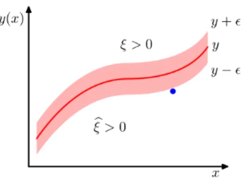
2.3. Support Vector Machines 15
Figure 2.3.4: Image from Bishop’s book [10, Chapter 7.1]: The regressor plane is shown in red as well as the -tube. Slack variables ξ,ξˆare also represented. Pointsxi above the
-tube have ξ >0, points inside the tube haveξ = ˆξ= 0, points below the -tube ˆξ >0.
2.3.2 Analysis
In Subsection 2.3.1 we have shown the problems that motivate the SVMs. A similar optimization problem is obtained both for regression and classification. We can define the following concepts now.
Definition 2.3.1 (SVC Problem). Given a classification problem
{(x1, l1), . . . ,(xM, lM)}, xi∈ X ⊂Rd, l∈ {−1,1},
the corresponding optimization problem is
arg min w,b,ξ J(w, b, ξ) =C M X i=1 ξi+1 2||w|| 2 s.t. li(w·xi+b)≥1−ξi, i= 1, . . . , M, ξi ≥0, i= 1, . . . , M . (2.3.4)
Definition 2.3.2 (SVR Problem). Given a regression problem,
{(x1, t1), . . . ,(xM, tM)}, xi ∈ X ⊂Rd, ti ∈R,
the corresponding optimization problem is
arg min w,b,ξ,ξˆ J(w, ξ) =C M X i=1 (ξi+ ˆξi) + 1 2||w|| 2 s.t. w·xi+b≥ti−−ξi, i= 1, . . . , M , w·xi+b≤ti++ ˆξi, i= 1, . . . , M , ξi,ξˆi≥0, i= 1, . . . , M . (2.3.5)
Both problems are similar but have some differences too. However, it is possible to define a formulation that unify both problems. We first show the unifying formulation. Definition 2.3.3 (Primal SVM Problem). Given a sample
a SVM problem is the following optimization problem, arg min w,b,ξ J(w, b, ξ) =C N X n=1 ξi+1 2||w|| 2 s.t. yi(w·xi+b)≥pi−ξi, i= 1, . . . , N, ξi ≥0, i= 1, . . . , N . (2.3.6)
With this definition it is easy to check the following proposition.
Proposition 2.3.1. The problem (2.3.6) is equivalent to (2.3.4) when choosing M = N
and
yi=ti, pi= 1i= 1, . . . , N ;
and it is also equivalent to (2.3.5) when we chooseN = 2M and we select
yi= 1, pi=ti−, i= 1, . . . , M
yM+i=−1, pM+i=−ti−, i= 1, . . . , M .
The unified problem defined in (2.3.6) is advantageous because we can use it to make an analysis that is valid for both SVC and SVR at the same time. We have reached a point then, where we have a single optimization problem, to which we can apply the optimization theory previously explained. In first place, notice that the problem (2.3.6) has a convex objective function and affine restrictions; thus, we can apply the Strong Duality Theorem 2.2.4. It is interesting then to obtain its dual problem, and in consequence, its Lagrangian. The Lagrangian of the primal SVM problem is
L(w, b, ξ, α, β) = 1 2||w|| 2+C N X i=1 ξi − N X i=1 αi(yi(w·xi+b)−pi+ξi)− N X i=1 βiξi, α, β≥0, (2.3.7) where α= (α1, . . . , αN), β = (β1, . . . , βN) .
Since we want to obtain the dual function, that is Θ(α, β) = min
w,b,ξL(w, b, ξ, α, β),
we have to compute the following derivatives:
∂L ∂w =w− N X i=1 αiyixi (2.3.8) ∂L ∂b = N X i=1 αiyi (2.3.9) ∂L
2.3. Support Vector Machines 17 Then, making ∂L ∂w = 0 we get w∗= N X i=1 αiyixi , (2.3.11)
which gives us a relation between the primal variable w and the dual variable α. Making
∂L ∂b = 0 we get N X i=1 αiyi= 0, (2.3.12)
which gives us a condition over the dual variable α, this is called the equality constraint. Finally, making ∂ξ∂L
i we have the conditionαi+βi =C, which, alongside the feasibility of
α and β gives 0 ≤αi ≤C, that is called the equality constraint. Using this conditions we can write the dual function as follows,
Θ(α) =L(w∗, b∗, ξ∗, α, β) = 1 2h N X i=1 αiyixi, N X j=1 αiyjxji − N X i=1 αiyi N X j=1 αjyjxj ·xi+ N X i=1 pi =−1 2 N X i=1 N X j=1 αiαjyiyjxi·xj+ N X i=1 αipi .
Then, since the dual function is maximized, the Dual Problemis the next one,
min α Θ(α) = 1 2 N X i=1 N X j=1 αiαjyiyjxi·xj− N X i=1 αipi
s.t. 0≤αi ≤C, i= 1, . . . , N (box constraint), N
X
i=1
yiαi = 0, (equality constraint).
(2.3.13)
The objective function Θ(α) of the Dual Problem is quadratic, hence it is convex on α. Moreover, the constraints over α are affine and simpler than in the Primal Problem. With these properties, it is sensible to say that solving the Dual Problem is an easier task than solving the primal one. Using the Strong Duality Theorem, it is sufficient to find a solution of the dual α∗ and then Θ(α∗) = f(w∗). Moreover, using the equation (2.3.11) we can recover the primal solution from the dual one. To find the solution of the dual problem, we use the KKT Theorem [9], for which we need first to write the KKT conditions, which are αi ≥0, (2.3.14) yi(w·xi+b)−pi+ξi ≥0, (2.3.15) αi(yi(w·xi+b)−pi+ξi) = 0, (2.3.16) βi ≥0, (2.3.17) ξi ≥0, (2.3.18) βiξi = 0, (2.3.19) αi+βi =C . (2.3.20)
Notice that α is only present in the three first conditions and the last, while β is present in the last four. And moreover, the dual problem only depends on α. However α and β
are connected by Equation (2.3.20); so givenα∗i, the value for βi∗ isC−α∗i. Our goal then, is to find α∗ that fulfills the first three KKT conditions. To do so, some algorithms have been developed, the most popular one, named the SMO algorithm, will be presented in the following section. However, before showing the method to find the solution, it is interesting to analyze some properties of this solution. In first place, notice that the primal solution
w∗ depends on the dual solution in the following way
w∗=
N
X
i=1
yiα∗ixi ;
however, the conditions (2.3.16) and (2.3.15) implies that any point xi of the sample such that yi(w·xi +b)−pi +ξi > 0 has an associated αi = 0 .Then, w∗ depends only on a subset of the points I={i: yi(w·xi+b)−pi+ξi = 0}, that is
w∗=X
i∈I
yiα∗ixi .
It is clear that the solution of the optimization problem depends only on the vectors xi
such thati∈I and thusαi >0, these points receive the name ofSupport Vectors and that
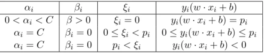
is the reason these models are namedSupport Vector Machines. It is relevant to study the properties of these support vectors. Using the KKT conditions, we can classify theSupport Vectors in terms of the value ofαi. This classification is shown in Table 2.3.1.
αi βi ξi yi(w·xi+b)
0< αi < C β >0 ξi= 0 yi(w·xi+b) =pi αi =C βi= 0 0≤ξi < pi 0≤yi(w·xi+b)≤pi αi =C βi= 0 pi < ξi yi(w·xi+b)<0
Table 2.3.1: Classification of Support Vectors in terms of the value of αi.
In order to interpret Table 2.3.1 we will focus first on classification wherepi = 1. In that
case, the first row indicatesyi(w·xi+b) = 1; that means that the vector is correctly classified and just on the margin of the model. The second row indicates 0≤yi(w·xi+b)≤1; that is
a point that is correctly classified but inside the margin. Finally, the last row characterizes the vectors that are misclassified. An example is shown in Figure 2.3.5.
The same analysis can be done with the regression problem, for the sake of concision we will see the case where yi = 1 and pi =ti−. In that case the first row characterizes the vectorsxi withw·xi+b=ti−; that is, those in the lower margin of the-tube. The second row is 0 ≤w·xi+b < ti−, which are the points below the-tube. Finally the
last row is w·xi+b <0< ti−which are also below the tube. In conclusion, the solution of the SVM optimization problem depends on those points that are “extreme”, those that are not easy to classify or to find a regressor plane for.
2.3.3 Kernel Trick
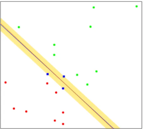
Until now we have seen the SVMs as linear models. Moreover, their initial motivation was to find maximum separability in linearly separable problems. Linear separability has the inconvenient of being unlikely in real world data. However, the following statement based on the Theorem proved by Cover [11] helps in this issue.
2.3. Support Vector Machines 19
Figure 2.3.5: The blue line shows the optimal separating plane, the shaded region is the maximum separation between the two classes. Support Vectors are shown in blue.
A complex pattern-classification problem, cast in a high-dimensional space non-linearly, is more likely to be linearly separable than in a low-dimensional space, provided that the space is not densely populated.
This statement is really useful: we just need to map the original features xi into a high-dimesional space (even infinite-dimensional)F through some mapping functionφ(x). Then, the SVM primal problem can be written as
arg min w,b,ξ J(w, b, ξ) =C N X n=1 ξi+1 2||w|| 2 s.t. yi(w·φ(xi) +b)≥pi−ξi, i= 1, . . . , N, ξi ≥0, i= 1, . . . , N , (2.3.21)
where w ∈ F. However, the complexity and computational cost of solving an optimiza-tion problem increases with the dimension of the feature space. Moreover, it would be intractable if F is infinite-dimensional. Nevertheless, SVMs have the property that their solution can be expressed in terms of the inner products of its patterns; therefore, we can use the kernel-induced feature spaces. This method of implicitly mapping the initial features in a high-dimensional space is called the Kernel Trick. In first place we choose a kernel function k(x, y); by Mercer’s Theorem 2.1.1 there exists an associated mapping φ. Then, the dual problem can be written as follows,
min α Θ(α) = 1 2 N X i=1 N X j=1 αiαjyiyjk(xi, xj)− N X i=1 αipi
s.t. 0≤αi ≤C, i= 1, . . . , N (box constraint), N
X
i=1
yiαi= 0, (equality constraint),
(2.3.22)
where k(xi, xj)) =φ(xi)·φ(xj). Moreover, the classification of a point xj requires com-puting w·φ(xj); using (2.3.11) the solution is the following:
w·φ(xj) =X
i∈I
yiαiφ(xi)·φ(xj) =X
i∈I
For findingb, we know that for xj, j∈ I such that ξj = 0 we have yj(w·φ(xj) +b) =pj, then we can get b as
b=pj/yj−w·φ(xi) =pj/yj −
X
i∈I
yiαik(xi, xj).
2.4
SMO Algorithm
In the previous section it has been shown that SVMs have multiple desirable properties such as the maximal separability and the possibility of applying thekernel trick. However, it is still necessary to develop a method required for training the SVMs. In this work we will focus on the SMO algorithm [12].
2.4.1 Update Step
In first place, it is important to state that SMO solves the Dual Problem (2.3.13); thus, using (2.3.22) it solves the Primal Problem (2.3.21) as well. That is, using the optimization theory presented in Section 2.2, SMO aims to find
α∗ = (α∗1, α∗2, . . . , α∗N)
that fulfills the KKT conditions, and therefore is an optimal solution. Then, using
w∗=X
i∈I
yiα∗iφ(xi),
where I are the indices of the Support Vectors and
b∗ =pj/yj−
X
i∈I
yiα∗ik(xi, xj)
for any j∈ I, it finds the optimal solution to the Primal Problem. In order to findα∗ the idea is to begin with an initial α(0) =~0; then we updateα(τ), that is, the vectorα at the iteration τ, as follows
α(τ+ 1) =α(τ) +δ(τ),
in a way that the update maximizes
Θτ−Θτ+1 = Θ(α(τ))−Θ(α(τ + 1)) = Θ(α(τ))−Θ(α(τ) +δ(τ)).
In order to find such update δ(τ), the easiest solution would be to update a single value
αi at a time; however, the Dual Problem includes the equality constraint N
X
i=1
yiαi = 0,
and updating a single αi will break the constraint. For that reason, the simplest update
that fulfills the constraint involves two coefficients. That is, first we select U, Lwith some heuristic rule that we study in Subsection 2.4.2; then, given the indices U, L we make the following update,
αU(τ + 1) =αU(τ) +δU(τ) αL(τ + 1) =αL(τ) +δL(τ),
2.4. SMO Algorithm 21
and we have to ensure
N
X
i=0
αi(τ+ 1)yi = 0.
It is possible then to connect δL(τ) and δU(τ). To do this we use the equality constraint
in times τ and τ+ 1, which can be written as follows
(τ) :αU(τ)yU +αL(τ)yL+ X i6=U,L αi(τ)yi = 0; (τ + 1) :αU(τ + 1)yU+αL(τ + 1)yL+ X i6=U,L αi(τ+ 1)yi = (αU(τ) +δU(τ))yU+ (αL(τ) +δL(τ))yL+ X i6=U,L αi(τ + 1)yi= 0.
Therefore, using the first equation and the last one, it is easy to see that
δU(τ)yU+δL(τ)yL= 0. (2.4.1) Using this equation it is possible to express the difference Θτ−Θτ+1 in terms of just δL,
and we have Θτ −Θτ+1= 1 2α(τ) tQα(τ)−pα(τ)− 1 2α(τ + 1) tQα(τ + 1)−pα(τ+ 1) = 1 2α(τ) tQα(τ)−pα(τ) − 1 2(α(τ) +δ(τ)) tQ(α(τ) +δ(τ))−p(α(τ) +δ(τ)) =−1 2 δ(τ) tQδ(τ) +α(τ)tQδ(τ) +δ(τ)tQα(τ) +pδ(τ) =−1 2δ(τ) tQδ(τ)− δ(τ)tQα(τ)−pδ(τ) , (2.4.2)
where p corresponds to the unifying formulation introduced in (2.3.21). Since it can be expressed with variables corresponding only to time τ, the iteration time can be omitted resulting in the following equation
Θτ−Θτ+1 =−1 2δ tQδ−δtQαˆ −pδ=−1 2A−B . (2.4.3) where α= (α1, α2, . . . , αN)t and δ = (0, . . . ,0, δL,0, . . . ,0, δU,0. . . ,0)t,
where only the positions L and U are not null. Given these clarifications, (2.4.3) can be further expanded. The term denoted as Acan be expressed as follows
A=δtQδ
=δU2QU U + 2δUδLQU L+δ2LQLL
=δL2φ(xU)·φ(xU) + 2(−yUyLδL)δLyUyLφ(xU)·φ(xL) +δL2φ(xL)·φ(xL) =δL2kφ(xU)k2−2δ2Lφ(xU)·φ(xL) +δL2kφ(xL)k2
Besides, we can develop the term B in the following way, B=δQα−pδ=δL((Qα)L−pL) +δU((Qα)U −pU) =δL N X i=1 QLiαi−pL ! +δU N X i=1 QU iαi−pU ! =δL N X i=1 QLiαi−pL ! −yUyLδL N X i=1 QU iαi−pU ! =yLδL yL N X i=1 QLiαi−pL ! −yU N X i=1 QU iαi−pU !! .
Moreover, the gradient of the dual objective function is the following
∇Θ(α) =Qα−p; (2.4.4)
therefore the position j of the gradient is
∇Θ(α)j =Qjα−pj = N X i=1 Qjiαi−pj ! .
Using this, the following is true:
B =yLδL(yL(∇Θ)L−yU(∇Θ)U) .
Finally, using the results for Aand B, the difference of the dual objective function can be expressed as follows: Θτ −Θτ+1=−yLδL(yL(∇Θ)L−yU(∇Θ)U)−1 2δ 2 Lkφ(xU)−φ(xL)k 2 =−ψ(δL). (2.4.5)
With this definition, the goal is to minimize ψ(δL), and since it is a convex function it is
sufficient to find δL∗ such thatψ0(δL∗) = 0 where
ψ0(δL) =yL(yL(∇Θ)L−yU(∇Θ)U) +δLkφ(xU)−φ(xL)k2 .
The result is the following
δ∗L= yL(yU(∇Θ)U−yL(∇Θ)L) kφ(xU)−φ(xL)k2 . (2.4.6) Defining ¯λas ¯ λ= (yU(∇Θ)U−yL(∇Θ)L) kφ(xU)−φ(xL)k2 ,
then the update of the dual variables αU and αL would the following ατL+1=ατL+yL¯λ
ατU+1=ατU−yUλ¯;
however, it is necessary to clip ¯λin order to keep the dual variables in the feasible region, that is 0≤αU, αL≤C. To achieve this, the update is defined in the following way
λ= min (C−ατL,λ¯) if yL = 1, λ= min (ατL,¯λ) if yL = -1, λ= min (ατU,λ¯) if yU = 1, λ= min (C−ατU,¯λ) if yU = -1.
2.4. SMO Algorithm 23
Then, we use λto update the dual variables
ατL+1=ατL+yLλ , ατU+1=ατU−yUλ .
It can be seen that even with the clipping, the update makes Θ smaller. To check just one case, set yL=−1 and ατL<λ¯, thenδLτ =yLατL, therefore
Θτ −Θτ+1=ψ(yLατL) =αLτ (yU(∇Θ)U −yL(∇Θ)L)−1 2(α τ L) 2k φ(xU)−φ(xL)k2 ≥ατL(yU(∇Θ)U −yL(∇Θ)L)>0.
The last inequality has not been seen yet since it is dependent on the election ofU and L. In the next subsection a heuristic rule is developed to select U and L, and moreover we prove the last inequality.
2.4.2 Selection Step: Selecting the Optimal (U, L)
Before presenting the heuristic methods that are used in the selection step it is important to recall the KKT conditions of this optimization problem, which are
αi ≥0, yi(w·φ(xi) +b)−pi+ξi ≥0, αi(yi(w·φ(xi) +b)−pi+ξi) = 0, βi ≥0, ξi ≥0, βiξi = 0, αi+βi =C .
The KKT conditions are important because given a tuple (w∗, b∗, ξ∗, α∗, β∗) that fulfills the KKT conditions, then the tuple (w∗, b∗, ξ∗) is the optimal solution of the primal and (α∗, β∗) is the optimal solution of the dual. In order to have an easier condition to check optimality the following Lemma can be proved.
Lemma 2.4.1. Define the following sets
IU+={i:yi= 1∧αi >0}, IU− ={i:yi =−1∧αi< C}, IL+={i:yi= 1∧αi < C}, IL− ={i:yi =−1∧αi >0},
and also define
IU =IU+∪IU−, IL=IL+∪IL−;
then, if the KKT conditions hold,
w·φ(xu)−yupu ≤ −b≤w·φ(xl)−ylpl, ∀u∈IU, ∀l∈IL. (2.4.7)
Proof. The two cases 0 ≤ αi < C and 0 < αi ≤ C are proved separately. Note that although the two sets are not disjoint, every αi is covered in one of them. The first case
is the following: αi < C =⇒ βi >0 =⇒ ξi = 0 , which can be followed from the KKT
conditions; then
that is
w·φ(xi)−yipi ≥ −bifyi = 1 (IL+), w·φ(xi)−yipi ≤ −bifyi =−1 (IU−).
The second case is the following: αi >0 =⇒ yi(w·φ(xi)−yipi+b)−pi+ξi = 0, which
can be followed from the KKT conditions; then
yi(w·φ(xi)−yipi+b)−pi ≤0 ;
that is
w·φ(xi)−yipi ≤ −bifyi = 1 (IU+), w·φ(xi)−yipi ≥ −bifyi =−1 (IL−).
This lemma provides an easy two-step rule for selecting (U∗, L∗); that is, the indices to update. The rule consists on selecting the pair of indices (U, L) that violate the most the KKT conditions. More formally, notice first the following:
Θ(α) = 1 2hw ∗ , N X i=1 αiyiφ(xi)i − N X i=1 αipi;
then taking derivatives with respect to αi the result is
(∇Θ(α))rj = ∂Θ(α)
∂αi
=hw∗, yiφ(xi)i −pi .
Therefore, multiplying the partial derivative times yi we get
yi(∇Θ(α))rj =yi ∂Θ(α)
∂αi =hw
∗, φ(x
i)i −yipi ;
thus, the condition of the equation (2.4.7) can be written as
yu(∇Θ(α))u ≤yl(∇Θ(α))l, ∀u∈IU, ∀l∈IL.
Given this result, we define ∆ as ∆(α) = max
u∈IU
(yu(∇Θ)u)−min
l∈IL
(yl(∇Θ)l) ;
this definition implies that if ∆(α)≤0, then by the Lemma 2.4.1,αis the optimal solution. However, if ∆(α)>0 then the KKT conditions are not met and thereforeα is not optimal. Moreover any pair u∈IU , l∈IL such that
yu(∇Θ(α))u−yl(∇Θ(α))l>0
is called a ’violating pair’. With this information, the heuristic rule used is to selectU∗, L∗
in the following way:
U∗= arg max u∈IU (yu(∇Θ)u), L∗= arg min l∈IL (yl(∇Θ)l). (2.4.8)
2.4. SMO Algorithm 25
Given the definition of the selection rule, it shows that the indices selected are those that most violate the KKT conditions and thus the rule is called ‘maximal violating pair’ rule. The first part of this subsection is focused on the definition of ‘violating pair’ and moreover, it provides the motivation for the ‘maximal violating pair’ rule. However, a better selection can be made. In first place, recall that the main goal to achieve a faster convergence is to minimize
Ψ(δ) = ∆Θ(α) = Θ(α+δ)−Θ(α),
which, using (2.4.2), can be written as
Ψ(δ) = ∆Θ(α) = Θ(α+δ)−Θ(α) = 1
2δ(τ)
tQδ(τ)− δ(τ)tQα(τ) +pδ(τ)
.
Moreover, using the derivatives of Θ(α) which are
∇Θ(α) =αtQ+p ,
∇2Θ(α) =Q ,
we can write Ψ(δ), which is quadratic, in the following way
Ψ(δ) = ∆Θ(α) = Θ(α+δ)−Θ(α) =∇Θ(α)δ+1 2δ
t∇2Θ(α)δ .
We have already seen in (2.4.5) that it can be expressed just in terms of δL:
Ψ(δ) =ψ(δL) =yLδL(yL(∇Θ)L−yU(∇Θ)U) +1 2δ 2 L kφ(xU)−φ(xL)k2 .
It is clear that although the function to optimize is dependent on the first and second order derivatives of Θ(α), with the maximal violating pair rule we are only using information about the first derivative ∇Θ(α). Nevertheless, Equation (2.4.6) gives us a closed solution for the optimal updateδ∗in terms of (U, L); then, our goal is to choose (U, L) that minimize Ψ(δ∗). To do that the following proposition can be used.
Proposition 2.4.1. Let (U, L) be a violating pair, then Ψ(δ) has the optimal value
−1 2
(yU(∇Θ)U−yL(∇Θ)L)2 kφ(xU)−φ(xL)k2
. (2.4.9)
Proof. With the optimalδL∗ obtained in (2.4.6) we just need to compute Ψ(δ∗) =ψ(δ∗L),
ψ(δL∗) =yLδ∗L(yL(∇Θ)L−yU(∇Θ)U) + 1 2(δ ∗ L)2 kφ(xU)−φ(xL)k2 =yL yL(yU(∇Θ)U−yL(∇Θ)L) kφ(xU)−φ(xL)k2 (yL(∇Θ)L−yU(∇Θ)U) + 1 2 yL(yU(∇Θ)U−yL(∇Θ)L) kφ(xU)−φ(xL)k2 2 kφ(xU)−φ(xL)k2 =−1 2 yL(yU(∇Θ)U−yL(∇Θ)L) 2 kφ(xU)−φ(xL)k2 ! .
Using Proposition 2.4.1 it is sufficient to choose (U, L) as a violating pair that min-imizes (2.4.9). However, this method requires a quadratic search. The solution, called
Second Order SMO [13], is to select a violating pair (U, L) in the following way:
U∗= arg max u∈IU (yu(∇Θ)u), L∗= arg min l∈IL −(yU(∇Θ)U−yL(∇Θ)L) 2 kφ(xU)−φ(xL)k2 ! . (2.4.10)
By selecting (U, L) in this way, the cost is linear since both steps consist of a linear cost search.
Both selections, (2.4.8) and (2.4.10), make use of the information of the gradient. It is clear then, that it is necessary to maintain the entire gradient ∇Θ in order to perform the indices selection. To do this, we use the following equation,
∇Θ(α)j =Qjα−pj = N X i=1 Qjiαi−pj ! .
Then, the initial gradient is (∇Θ)0=~0, and at iterationτ we have the gradient
∇Θ(α)τj =Qjατ −pj = N X i=1 Qjiατi −pj ! ,
whereQjis thej-th row of Q. Using this gradient we perform the selection step at iteration τ+ 1 obtainingU, Land then we perform the update step, obtaining αU(τ+ 1), αL(τ+ 1).
Then, we can express the update of the gradient in a simple way. We first compute the difference between ∇Θ(α)τ+1 and ∇Θ(α)τ, that is,
∇Θ(α)τ+1− ∇Θ(α)τ =
N
X
i=1
Qjiδiτ =QjUδτU+QjLδτL.
Then, we have the following difference,
∇Θ(α)τ+1− ∇Θ(α)τ =Qδτ ;
therefore, to update the gradient we just have to make ∇Θ(α)τ+1=∇Θ(α)τ +Qδτ .
2.4.3 Computational Cost
With both the update and selection step explained, it is necessary to write the whole algorithm and analyze its computational cost. To do so, Second Order SMO is given in Algorithm 1. In order to get the computational cost of the Second Order SMO algorithm we will study the cost of each iteration. In first place, the selection step consists on two linear cost searches, that have a O(2N) cost. Then, the Update Step requires just some comparisons and has cost O(1). Also, the Gradient Update requires the multiplication of the matrix Q and the vector δ, where δ is null except for the positions U, L; that means that it has a cost O(2N). Finally, the computation of ∆ requires to check the conditions of IU and IL for the recently updated variables αU and αL, that is, a O(1) cost. Therefore, putting it all together, the computational cost of each iteration of SMO
2.4. SMO Algorithm 27
Algorithm 1:SMO
Data: matrix Q, vectorp, parameterC
Result: vector α∗ α←~0 ;
∇Θ← −p ;
IU ← {i:yi= 1∧αi >0} ∪ {i:yi =−1∧αi< C} ; IL← {i:yi = 1∧αi < C} ∪ {i:yi=−1∧αi >0} ;
∆ = maxu∈IU(yu(∇Θ)u)−minl∈IL(yl(∇Θ)l) ; // KKT conditions
while∆> toldo
U = arg maxu∈IU(yu(∇Θ)u) ; // Selection Step L= arg minl∈IL −(yU(∇Θ)U−yl(∇Θ)l) 2 QU U−2QU l+Qll ; // Selection Step λ← (yU(∇Θ)U−yL(∇Θ)L) QU U−2QU L+QLL ; if yL== 1 thenλ= min(C−αL, λ); elseλ= min(αL, λ); if yU == 1 thenλ= min(αU, λ);
elseλ= min(C−αU, λ);
αL←αL+yLλ;αU ←αU−yUλ; // Update Step δ=~0 ; δ[L]←yLλ;δ[U]← −yUλ; ∇Θ← ∇Θ +Qδ ; // Gradient Update IU ← {i:yi= 1∧αi < C} ∪ {i:yi =−1∧αi < C} ; IL← {i:yi = 1∧αi >0} ∪ {i:yi =−1∧αi>0};
∆←maxu∈IU(yu(∇Θ)u)−minl∈IL(yl(∇Θ)l) ; // KKT conditions
is O(2N). Moreover, in [14] it has been proven that with this Selection Step the, after a some finite number of iterations, the convergence of the algorithm is linear. In order to get a solution we need to find a number of support vectors that is tipically proportional to the size of the sample; therefore, updating two variables per iteration, at least O(N) iterations are necessary. Since the cost of each iteration is also linear, it is said that the total cost of
Second Order SMO is larger than a cost O(N2), and sometimes it is said to have a cost
![Figure 2.3.1 : Image from Bishop’s book [10, Chapter 7.1].: The plane y(x) = wx + b = 0 is shown in red](https://thumb-us.123doks.com/thumbv2/123dok_us/9911333.2484321/28.892.323.572.124.323/figure-image-bishop-book-chapter-plane-shown-red.webp)
![Figure 2.3.2 : Image from Bishop’s book [10, Chapter 7.1]: There are points of two classes, blue is 1 and yellow is −1](https://thumb-us.123doks.com/thumbv2/123dok_us/9911333.2484321/29.892.335.558.126.332/figure-image-bishop-book-chapter-points-classes-yellow.webp)
![Figure 2.3.3 : Image from Bishop’s book [10, Chapter 7.1]: The quadratic error is shown in green and the function defined as ˆ e in red.](https://thumb-us.123doks.com/thumbv2/123dok_us/9911333.2484321/30.892.327.565.132.272/figure-image-bishop-chapter-quadratic-error-function-defined.webp)