E
MPIRICAL LIKELIHOOD BASED INFERENCE
UNDER COMPLEX SAMPLING DESIGNS
Yves G. BERGER1, University of Southampton, UK
Resum´
e
L’approche propos´ee permet d’estimer de mani`ere consistante des param`etres qui sont solutions d’´equations estimantes (par exemple: moyennes, totaux, quantiles, corr´elation, param`etres de r´egressions (non)lin´eaire). L’approche propos´ee a l’avantage de permettre de construire des intervalles de confiance sans devoir estimer la variance. Ces inter-valles de confiance ne sont pas bas´es sur la normalit´e de l’estimateur ponctuelle. La lin´earisation, le r´e-´echantillonnage (jackknife ou bootstrap) ou les probabilit´es d’inclusion d’ordre deux ne sont ´egalement pas n´ecessaires, mˆeme dans le cas ou le param`etre d’int´erˆet n’est pas lin´eaire. Cette approche donne des intervalles de confiance consistants mˆeme si la distribution d’´echantillonnage est asym´etriques (par exemple, pour des domaines ou en pr´esence de valeurs extrˆemes), ou lorsque la lin´earisation ne donne pas de bon estim´es de variance. L’approche propos´ee permet aussi d’estimer des param`etres de mod`eles de r´egressions g´en´eralis´ees (par exemple, la r´egression logistique) et de tester s’ils sont sig-nificatifs, sous une approche bas´ee sur le plan d’´echantillonnage. L’information auxiliaire peut ˆetre tenue en compte de mani`ere naturelle et tr`es simple, sans faire appel `a aucune technique de calage et sans perte de pr´ecision. L’approche bas´ee sur la vraisemblance empirique est une approche bas´ee sur le plan d’´echantillonnage. Un mod`ele de super-population n’est pas n´ecessaire. L’approche propos´ee est diff´erente de l’approche bas´ee sur la pseudo vraisemblance empirique [6].
Abstract
The approach proposed gives design-consistent estimators of parameters which are so-lutions of estimating equations (e.g. averages, totals, quantiles, correlation, (non)linear regression parameters). It can be used to construct confidence intervals without variance estimates. These confidence intervals are not based on the normality of the point esti-mator. Linearisation, re-sampling (jackknife or bootstrap) or joint-inclusion probabilities are not necessary, even when the parameter of interest is not linear. This approach gives consistent confidence intervals even when the sampling distribution is skewed (e.g. with domains or with outlying values), or when linearisation gives biased variance estimates. The proposed approach can be used to estimate generalised regression parameters (e.g.
logistic regression) and to test if they are significant, under a design-based approach. The auxiliary information is naturally taken into account, without the need of a calibra-tion distance funccalibra-tion. The empirical likelihood approach is a design-based approach. A super-population model is not necessary. The empirical likelihood approach proposed is different from the pseudoempirical likelihood approach [6].
Keywords
Confidence intervals, Estimating equations, Regression estimator, Stratification, Unequal inclusion probabilities.
1
Introduction
LetU be a finite population of N units; whereN is not necessarily known. Suppose that the population parameter of interest θN is the unique solution of the following estimating equation (see [8]).
G(θ) = 0, with G(θ) = X
i∈U
gi(θ), (1)
where gi(θ) is a function of θ and of the characteristics of the uniti, such as the variables
of interest and the auxiliary variables. This function does not need to be differentiable. The aim is to compute a maximum empirical likelihood point estimate and a confidence interval for θN. Suppose that we have a sample s of size n selected randomly using a sampling design. The πi shall denote the first-order inclusion probabilities. We adopt
a non-parametric design-based approach; where the sampling distribution is specified by the sampling design and where θN and the values of the variables are fixed (non-random) quantities. We consider a single stage design. The approach proposed can be generalised for multi-stage design (see § 3 and [3])
In § 2, the approach proposed by Berger & De La Riva Torres [3] is described. In § 4, we presents extensions of this approach. In § 3, we have an illustration based on the European Union Statistics on Income and Living Conditions (EU-SILC) survey.
2
Empirical likelihood approach
Let zi be the values of the design (or stratification) variables defined by
zi = (zi1, . . . , ziH)> and where n= (n1, . . . , nH)> (2)
denotes the vector of the strata sample sizes, with zih = πi when i ∈ Uh and zih = 0
otherwise.
Let vector xi be the vector containing the values of auxiliary variables for unit i. Let
fi(xi,ϕN) be known vector function of xi and ϕN, where ϕN is a fixed and known vector of parameters which is defined as the solution of
X
i∈U
For example, if the population means µx = N−1P
i∈Uxi are known, ϕN = µx and
fi(xi,ϕN) = xi−ϕN. The most common situation is practice is to know a set of totals, means or proportions from large external censuses or surveys. The vectorϕN may contains simultaneously totals, means, proportions or quantiles. The functions fi(xi,ϕN) need to be defined accordingly.
Consider the following empirical log-likelihood function
`(m) = log Y i∈s mi ! =X i∈s log(mi), (4) where Q i∈s and P
i∈s denote the product and the sum over the sampled units. The
quantities mi are unknown positive scale loads [10] which shall be estimated. Let mb
? i(θ)
be the values which maximise (4) subject to the constraints mi ≥0 and
X i∈s mic?i(θ) =C ?, (5) with c? i(θ) = (c >
i , gi(θ))> and C? = (C>,0)>, for a given θ. Here ci = (z>i ,fi(xi,ϕN)
>)>
and C = (n>,0>)>. Consider
`(mb?, θ) = X
i∈s
log(mb?i(θ)), (6)
which is the maximum value of the empirical log-likelihood function (4) subject to the constraint (5).
2.1
Maximum empirical likelihood point estimator
The maximum empirical likelihood estimate θbof θN is defined by the value of θ which maximises the empirical log-likelihood function `(mb?, θ) in (6). Berger & De La Riva
Torres [3] showed that bθ is simply the solution of b G(θ) = 0, with Gb(θ) = X i∈s b mi gi(θ), (7)
where the mbi are the values which maximise (4) subject to mi ≥ 0 and the reduced
constraint
X
i∈s
mici =C· (8)
The mbi are survey weights. Berger & De La Riva Torres [3] showed that the weights mbi are asymptotically optimal.
Note that the mbi are calibrated weights because Pi∈smbifi(xi,ϕN) = 0 (see (8) and the definition of ci before (6)). The calibration property is the consequence of the
maximi-sation of the empirical log-likelihood function (8), rather than a weighting technique. Calibration is achieved because the parameter ϕN is a known fixed parameter which does not need to be estimated from the empirical log-likelihood function. The focus is on the
maximisation of the empirical log-likelihood function rather than on weighting. The sur-veys weights appear naturally as the consequence of this maximisation.
Note that if we do not include the auxiliary information fi(xi,ϕN) within ci; that is, if
we use ci =zi and C =n, we obtain the Horvitz & Thompson [11] weights: mbi =π
−1
i .
When the parameter of interest is a total, we use gi(θ) =yi−n−1θπi and the maximum
empirical likelihood estimator is the Horvitz & Thompson [11] estimator: θb= P
i∈syiπi−1.
If the parameter of interest is a mean, we use gi(θ) = yi−θ, and the maximum empirical
likelihood estimator is the H´ajek [9] estimator of a mean: bθ = P i∈sπ −1 i −1P i∈syiπi−1.
The approach proposed is not limited to these estimators, as it can be used for any parameters which are defined as the solution of (1).
2.2
Empirical likelihood confidence intervals
Consider the empirical log-likelihood ratio function (or deviance) defined by b
r(θ) = 2{`(mb)−`(mb?, θ)}, (9) where`(mb) = P
i∈slog(mbi) is the maximum value of (4) under the reduced constraint (8). Berger & De La Riva Torres [3] show that br(θN) follows asymptotically a χ2-distribution with 1 degree of freedom when the sampling fraction is negligible, under a set of weak regularity conditions given in [3]. Thus, theα-level empirical likelihood confidence interval for the population parameter θN is given by
θ : br(θ)≤χ21(α) · (10)
where χ2
1(α) is the upperα-quantile of the χ2-distribution with 1 degree of freedom. The
p-value to test H0 : θN = θ0 is given by
R∞ b
r(θ0)f(x)dx, where f(x) is the density of the
χ2-distribution with 1 degree of freedom.
Note that br(θ) is a convex non-symmetric function with a minimum when θ is the maxi-mum empirical likelihood estimate θb. The confidence interval (10) can be found using a bisection search method. This involves calculating for several values of θ. The confidence interval (10) is asymmetric when the sampling distribution is asymmetric. In a series of simulation, Berger & De La Riva Torres [3] showed that the empirical likelihood confi-dence interval may give better coverages than standard conficonfi-dence intervals based on the central limit theorem and/or bootstrap.
3
An application to the European Union Statistics on
Income and Living Conditions (EU-SILC) survey
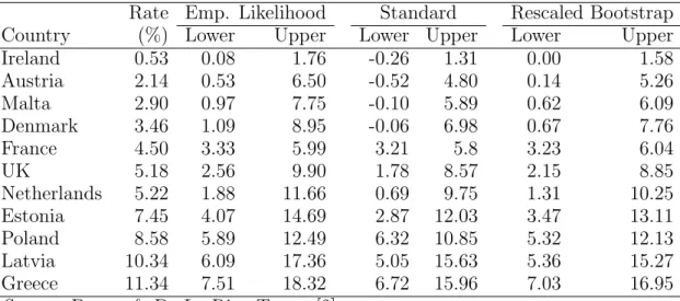
The approached described in § 2 is limited to single stage sampling. Berger & De La Riva Torres [3] show how it can be extended for multi-stage sampling designs using an ultimate cluster approach. This is the approach which was proposed for the EU-SILC survey. In this §, we report some numerical results which can be found in Berger & De La Riva Torres [2].Table 1: Persistent at-risk-of-poverty rate & confidence intervals. 2009 EU-SILC. Rate Emp. Likelihood Standard Rescaled Bootstrap Country (%) Lower Upper Lower Upper Lower Upper
Ireland 0.53 0.08 1.76 -0.26 1.31 0.00 1.58 Austria 2.14 0.53 6.50 -0.52 4.80 0.14 5.26 Malta 2.90 0.97 7.75 -0.10 5.89 0.62 6.09 Denmark 3.46 1.09 8.95 -0.06 6.98 0.67 7.76 France 4.50 3.33 5.99 3.21 5.8 3.23 6.04 UK 5.18 2.56 9.90 1.78 8.57 2.15 8.85 Netherlands 5.22 1.88 11.66 0.69 9.75 1.31 10.25 Estonia 7.45 4.07 14.69 2.87 12.03 3.47 13.11 Poland 8.58 5.89 12.49 6.32 10.85 5.32 12.13 Latvia 10.34 6.09 17.36 5.05 15.63 5.36 15.27 Greece 11.34 7.51 18.32 6.72 15.96 7.03 16.95
Source: Berger & De La Riva Torres [2].
The 2009 EU-SILC user database was used to estimate the persistent at-risk-of-poverty rate. An ultimate cluster approach was adopted, where the units are the primary sampling units. In the Table 1, we have the point estimate for several European countries. Several confidence intervals are reported: the empirical likelihood confidence intervals, the stan-dard confidence intervals based on variance estimates [e.g. 5] and the rescaled bootstrap confidences interval [19]. Note that the bounds of the standard intervals can be outside the range of the parameter space, as the lower bound are negative for Ireland, Austria, Malta and Denmark (the rates are always positive). The bootstrap bounds and the empirical likelihood bounds are larger than the bounds of the standard intervals. These differences are more pronounced for Austria, Malta, Denmark, the Netherlands, Estonia, Latvia and Greece. This is due to the skewness of the sampling distribution. The differences between these confidence intervals are more pronounced for domains. The results for domains are not presented here. They can be found in [2].
4
Discussion
The proposed approached can be generalised in numerous ways. Berger & De La Riva Torres [3] proposed a penalised empirical likelihood function to accommodate large sam-pling fraction. They also show how unit non-response and multi-stage samsam-pling can be taken into account (see [2] and § 7.3 in [3]).
The approach proposed is not limited to a single parameter. Oguz-Alper & Berger [14] generalised this approach to a vector of parameters. They show how profiling can be used to test and construct a confidence interval for a component of the vector of parameters. For example, with a generalised linear regression model, we may be interested in testing if a slope is significant. Profiling allows to test if a slope is significant. When building a model, it is necessary to compare two nested models. In this case, profiling can be used to test if the additional parameters are significant. Another example is when the parameter of interest is a correlation coefficient [e.g. 15, 17].
It is often the case that several surveys carried out from the same population, measure the same common variable. Population totals of these variables are often unknown. Kabzin-ska & Berger [13] proposed an empirical likelihood approach to align estimates obtained from these surveys. This approach ensures that both samples produce the same point estimates for the common variable. It also allows to incorporate additional benchmark constraints, constructed around known fixed parameters. The approach that is proposed by Kabzinska & Berger [13] can be used to construct confidence intervals.
Non-parametric bootstrap is an alternative approach which can be used to derive non-parametric confidence intervals. The consistency of the bootstrap confidence intervals is limited to smooth function of means and for quantiles with small sampling fractions [e.g. 20, Ch.6]. The direct bootstrap [1] is limited to variance estimation of totals, be-cause it provides a second-moment matching in this case. For complex parameters (such as quantiles), only simulation evidence are provided. Results on the consistency of the direct bootstrap confidence interval is not available. The proposed empirical likelihood confidence interval is consistent for a wider class of parameters (which are solution of estimating equations) with large and small sampling fractions (see [3]). The approach proposed is simpler to implement and less computationally intensive than the bootstrap, especially with calibration weights. From a practical point of view, bootstrap is usually preferred because it does not rely on analytic derivation. The proposed approach also possesses the same property. Like bootstrap, the proposed approach does not rely on analytic derivation. The simulation studies presented in [3] show that, for means and quantiles, bootstrap confidence intervals may have coverages and tail error rates signif-icantly different from their nominal levels. The empirical likelihood approach may give better coverages.
There are some analogies between the proposed empirical likelihood approach and calibra-tion [7, 12, 16]. Berger & De La Riva Torres [3] showed that empirical likelihood estimator is asymptotically equivalent to a calibrated regression estimator, where θN is a mean or a total. The objective function (4) is related to the concept of empirical likelihood and can be used with or without auxiliary information. The empirical likelihood approach gives calibrated weights because of the maximisation of the empirical log-likelihood func-tion. Furthermore, the objective function (4) is not a distance function, because it is not a function of the first-order inclusion probabilitiesπi. The advantage of the proposed
empirical likelihood approach over standard calibration [7] is the fact that (i) it gives positive weights that are asymptotically optimal (see [3]), (ii) the empirical log-likelihood ratio function (9) can be used to construct confidence intervals and to test hypotheses, (iii) and it can be used with complex parameters. Berger & De La Riva Torres [4] showed how the empirical likelihood approach can be used with any additional calibration dis-tance function.
Note that the empirical likelihood approach proposed is different from the pseudoempir-ical likelihood approach [6]. The pseudoempirpseudoempir-ical likelihood approach is not based on (4) and is based on the Kullback-Leibler distance. Pseudoempirical likelihood confidence intervals rely on variance estimates [21]. Unlike the pseudoempirical likelihood approach, the computation of the proposed confidence interval does not rely on variance estimates. This means that it can be applied to a wide class of parameters. The proposed approach is also simpler to implement than the pseudoempirical likelihood. The simulation studies
presented in Berger & De La Riva Torres [3] show that, for means, the empirical likeli-hood confidence interval may give better coverages than the pseudoempirical likelilikeli-hood confidence intervals.
The author is currently developing a R [18] package. More information will be available on the author’s web-page: http://yvesberger.co.uk. Some papers in the references’ list below can be downloaded from the author’s web-page.
References
[1] Antal, E., and Till´e, Y.A direct bootstrap method for complex sampling designs
from a finite population. Journal of the American Statistical Association 106 (2011), 534–543.
[2] Berger, Y. G., and De La Riva Torres, O. Empirical likelihood confidence
intervals: an application to the EU-SILC household surveys. Contribution to Sam-pling Statistics, Contribution to Statistics: F. Mecatti, P. L. Conti, M. G. Ranalli (editors). Springer (2014), 20pp.
[3] Berger, Y. G., and De La Riva Torres, O. An empirical likelihood approach
for inference under complex sampling design. To appear in the Journal of the Royal Statistical Society, Series B (2015), 22pp.
[4] Berger, Y. G., and De La Riva Torres, O. Empirical likelihood confidence
interval using complex survey weights. 60th session of International Statistical Insti-tute, Rio de Janeiro, Brasil (2015), 3pp.
[5] Berger, Y. G., and Priam, R. A simple variance estimator of change for rotating
repeated surveys: an application to the EU-SILC household surveys. To appear in the Journal of the Royal Statistical Society, Series A (2015), 22pp.
[6] Chen, J., and Sitter, R. R. A pseudo empirical likelihood approach to the
effective use of auxiliary information in complex surveys. Statistica Sinica 9 (1999), 385–406.
[7] Deville, J. C., and S¨arndal, C. E. Calibration estimators in survey sampling. Journal of the American Statistical Association 87, 418 (1992), 376–382.
[8] Godambe, V. P. An optimum property of regular maximum likelihood estimation.
The Annals of Mathematical Statistics 31, 4 (1960), pp. 1208–1211.
[9] H´ajek, J. Comment on a paper by D. Basu. in Foundations of Statistical Inference.
Toronto: Holt, Rinehart and Winston, 1971.
[10] Hartley, H. O., and Rao, J. N. K. A new estimation theory for sample surveys, ii. New Developments in survey Sampling (Johnson, N.L., and Smith, H.Jr., Eds.) Wiley, New York (1969), 147–169.
[11] Horvitz, D. G., and Thompson, D. J. A generalization of sampling without replacement from a finite universe. Journal of the American Statistical Association 47, 260 (1952), 663–685.
[12] Huang, E. T., and Fuller, W. A. Nonnegative regression estimation for survey
data. Proceedings Social Statistics Section American Statistical Association (1978), 300–303.
[13] Kabzinska, E., and Berger, Y. G. Aligning estimates from different surveys
using empirical likelihood methods. Proceeding of the conference on New Techniques and Technologies for Statistics. http://www.cros-portal.eu/sites/default/ files//Kabzinska_Aligning_estimates_from_different_surveys_using_EL_ methods.pdf, Brussels, 2015.
[14] Oguz-Alper, M., and Berger, Y. G. Empirical likelihood confidence
inter-vals and significance test for regression parameters under complex sampling designs. Proceedings of the Survey Research Method Section of the American Statistical As-sociation, Joint Statistical Meeting, Boston (2014), 10pp.
[15] Owen, A. B. Empirical likelihood ratio confidence regions. The Annals of Statistics
18, 1 (1990), 90–120.
[16] Owen, A. B. Empirical likelihood for linear models. The Annals of Statistics 19, 4
(1991), 1725–1747.
[17] Owen, A. B. Empirical Likelihood. Chapman & Hall, New York, 2001.
[18] R Development Core Team. R: A Language and Environment for Statistical
Computing. R Foundation for Statistical Computing. http://www.R-project.org, Vienna, Austria, 2014.
[19] Rao, J. N. K., Wu, C. F. J., and Yue, K. Some recent work on resampling
methods for complex surveys. Survey Methodology 18 (1992), 209–217.
[20] Shao, J., and Tu, D. The Jackknife and Boostrap. New York: Springer, 1996.
[21] Wu, C., and Rao, J. N. K. Pseudo-empirical likelihood ratio confidence intervals