PAC-Bayesian Theorems for Domain Adaptation with Specialization to Linear Classifiers

Specialization to Linear Classifiers

Pascal Germain, Amaury Habrard, Fran¸cois Laviolette, Emilie Morvant

To cite this version:

Pascal Germain, Amaury Habrard, Fran¸cois Laviolette, Emilie Morvant. PAC-Bayesian

The-orems for Domain Adaptation with Specialization to Linear Classifiers. [Research Report]

Universit´

e Jean Monnet, Saint-´

Etienne (42); D´

epartement d’Informatique et de G´

enie Logiciel,

Universit´

e Laval (Qu´

ebec); ENS Paris; IST Austria. 2016.

<

hal-01134246v3

>

HAL Id: hal-01134246

https://hal.archives-ouvertes.fr/hal-01134246v3

Submitted on 8 Aug 2016

HAL

is a multi-disciplinary open access

archive for the deposit and dissemination of

sci-entific research documents, whether they are

pub-lished or not.

The documents may come from

teaching and research institutions in France or

abroad, or from public or private research centers.

L’archive ouverte pluridisciplinaire

HAL

, est

destin´

ee au d´

epˆ

ot et `

a la diffusion de documents

scientifiques de niveau recherche, publi´

es ou non,

´

emanant des ´

etablissements d’enseignement et de

recherche fran¸

cais ou ´

etrangers, des laboratoires

publics ou priv´

es.

Specialization to Linear Classifiers

Pascal Germain

Amaury Habrard

Fran¸cois Laviolette

Emilie Morvant

´

Ecole Normale Sup´erieure, 75230 Paris, France

2

Univ Lyon, UJM-Saint-Etienne, CNRS, Institut d’Optique Graduate School, Laboratoire Hubert Curien UMR 5516, F-42023, Saint-Etienne, France

3 _{D´epartement d’informatique et de g´enie logiciel}

Universit´e Laval, Qu´ebec, Canada

August 8, 2016

This report is a long version of our paper entitled A PAC-Bayesian Approach for Domain Adaptation with Specialization to Linear Classifiers published in the proceedings of the International Conference on Machine Learning (ICML) 2013. We improved our main results, extended our experiments, and proposed

an extension to multisource domain adaptation.

Abstract

In this paper, we provide two main contributions in PAC-Bayesian theory for domain adaptation where the objective is to learn, from a source distribution, a well-performing majority vote on a different target distribution. On the one hand, we propose an improvement of the previous approach proposed by Germain et al. (2013), that relies on a novel distribution pseudodistance based on a disagreement averaging, allowing us to derive a new tighter PAC-Bayesian domain adaptation bound for the stochastic Gibbs classifier. We specialize it to linear classifiers, and design a learning algorithm which shows interesting results on a synthetic problem and on a popular sentiment annotation task. On the other hand, we generalize these results to multisource domain adaptation allowing us to take into account different source domains. This study opens the door to tackle domain adaptation tasks by making use of all the PAC-Bayesian tools.

1

Introduction

As human beings, we learn from what we saw before. Think about our education process: when a student attends to a new course, he has to make use of the knowledge he acquired during previous courses. However, in machine learning the most common assumption is based on the fact that the learning and test data are drawn from the same probability distribution. This strong assumption may be clearly irrelevant for a lot of real tasks including those where we desire to adapt a model from one task to another one. For instance, a spam filtering system suitable for one user can be poorly adapted to another who receives significantly different emails. In other words, the learning data associated with one or several users could be unrepresentative of the test data coming from another one. This enhances the need to design methods for adapting a classifier from learning (source) data to test (target) data. One solution to tackle this issue is to consider the domain adaptationframework1, which arises when the distribution generating the target data (thetarget domain) differs from the one generating the source data (thesource domain). In such a situation, it is well known that domain adaptation is a hard and challenging task even under strong assumptions (Ben-David and Urner, 2012; Ben-David et al.,2010b; Ben-David and Urner, 2014). Note that domain adaptation with learning data coming from different source domains is referred to as multisource or multiple sources domain adaptation (Crammer et al., 2007; Mansour et al., 2009c; Ben-David et al.,2010a).

Among the existing approaches in the literature to address domain adaptation, the instance weighting-based methods allow one to deal with the covariate-shift problem (e.g.,Huang et al.,2006;Sugiyama et al., 2008), where source and target domains diverge only in their marginals,i.e., they share the same labeling function. Another technique is to exploit self-labeling procedures, where the objective is to transfer the source labels to the target unlabeled points (e.g.,Bruzzone and Marconcini(2010);Habrard et al.(2013); Morvant (2014). A third solution is to learn a new common representation from the unlabeled part of source and target data. Then, a standard supervised learning algorithm can be executed on the source labeled instances (e.g.,Glorot et al.(2011);Chen et al. (2012)).

The work presented in this paper stands into a popular class of approaches, which relies on a distance between the source distribution and the target distribution. Such distance depends on the set H of hypotheses (or classifiers) considered by the learning algorithm. The intuition behind this approach is that one must look for a set Hthat minimizes the distance while preserving good performances on the source data; if the distributions are close under this measure, then generalization ability may be “easier” to quantify. In fact, defining such a measure to quantify how much the domains are related is a major issue in domain adaptation. For example, in the context of binary classification with the 0-1 loss function, Ben-David et al. (2010a); andBen-David et al. (2006) have considered theH∆H-divergence between the marginal distributions. This quantity is based on the maximal disagreement between two classifiers, allowing them to deduce a domain adaptation generalization bound based on the VC-dimension theory. The discrepancy distance proposed by Mansour et al.(2009a) generalizes this divergence to real-valued functions and more general losses, and is used to obtain a generalization bound based on the Rademacher complexity. In this context, Cortes and Mohri (2011, 2014) have specialized the minimization of the discrepancy to regression with kernels. In these situations, domain adaptation can be viewed as a multiple trade-off between the complexity of the hypothesis classH, the adaptation ability ofHaccording to the divergence between the marginals, and the empirical source risk. Moreover, other measures have been exploited under different assumptions, such as the R´enyi divergence suitable for importance weighting (Mansour et al.,2009b), or the measure proposed byC. Zhang(2012) which takes into account the source and target true labeling, or the Bayesian “divergence prior” (Li and Bilmes,2007) which favors classifiers closer to the best source model. However, a majority of methods prefer to perform a two-step approach:

(i)first construct a suitable representation by minimizing the divergence, then(ii) learn a model on the source domain in the new representation space.

The novelty of our contribution is to explore the PAC-Bayesian framework to tackle domain adap-tation in a binary classification situation without target labels (sometimes called unsupervised domain adaptation). Given a prior distribution over a family of classifiers H, PAC-Bayesian theory (introduced byMcAllester,1999) focuses on algorithms that output a posterior distributionρoverH(i.e., aρ-average over H) rather than just a single classifier h∈ H. Following this principle, we propose a pseudometric which evaluates the domain divergence according to theρ-average disagreement of the classifiers over the domains. This disagreement measure shows many advantages. First, it is ideal for the PAC-Bayesian set-ting, since it is expressed as aρ-average overH. Second, we prove that it is always lower than the popular

H∆H-divergence. Last but not least, our measure can be easily estimated from samples. Indeed, based on this disagreement measure, we derived in a previous work (Germain et al.,2013) a first PAC-Bayesian domain adaptation bound expressed as a ρ-averaging. In this paper, we provide a new version of this result, that does not change the philosophy supported by the previous bound, but clearly improves the theoretical result: The domain adaptation bound is now tighter and easier to interpret. Thanks to this new result, we also derive2 _{three new PAC-Bayesian domain adaptation generalization bounds. Then, in} contrast to the majority of methods that perform a two-step procedure, we design an algorithm tailored to linear classifiers, calledPBDA, which jointly minimizes the multiple trade-offs implied by the bounds. The first two quantities being, as usual in the PAC-Bayesian approach, the complexity of the majority vote measured by a Kullback-Leibler divergence and the empirical risk measured by the ρ-average errors on the source sample. The third quantity corresponds to our domain divergence and assesses the capacity of the posterior distribution to distinguish some structural difference between the source and target samples. Finally, we extend our results to domain adaptation with multiple sources by considering a mixture of different source domains as done byBen-David et al.(2010a).

The rest of the paper is structured as follows. Section 2 deals with two seminal works on domain adaptation. The PAC-Bayesian framework is then recalled in Section 3. Note that for the sake of com-pleteness, we provide for the first time the explicit derivation of the algorithm PBGD3(Germain et al., 2009a) tailored to linear classifiers in supervised learning. Our main contribution, which consists in a

2_{In this paper, we were very keen to improve the readability of our proofs, particularly those provided byGermain et al.}

domain adaptation bound suitable for PAC-Bayesian learning, is presented in Section4. Then, we derive our new algorithm for PAC-Bayesian domain adaptation in Section 5, that we experiment in Section6. Afterwards, we generalize this analysis to multisource domain adaptation in Section7. Before concluding in Section 9, we discuss two important points in Section 8: (i) two different results for the multisource setting that imply open-questions for deriving new algorithms, and(ii) the comparison between our new result and the one provided inGermain et al.(2013).

2

Domain Adaptation Related Works

In this section, we review the two seminal works in domain adaptation that are based on a divergence measure between the domains (Ben-David et al.,2010a;Ben-David et al.,2006;Mansour et al.,2009a).

2.1

Notations and Setting

We consider domain adaptation for binary classification tasks whereX ⊆Rdis the input space of dimension dand Y ={−1,+1} is the label set. Thesource domainPS and the target domainPT are two different

distributions over X×Y (unknown and fixed), DS and DT being the respective marginal distributions

over X. We tackle the challenging task where we have no target labels. A learning algorithm is then provided with alabeled source sample S={(xs

i, yis)}mi=1 consisting of mexamples drawni.i.d.3 fromPS,

and anunlabeled target sample T ={xt_j}m0

j=1 consisting ofm0 examples drawni.i.d. fromDT. Note that,

we denote the distribution of a m-sample by (PS)m. We suppose that His a set of hypothesis functions

for X to Y. Theexpected source error and the expected target errorof h∈ H overPS, respectively PT,

are the probability thatherrs on the entire distributionPS, respectivelyPT,

RPS(h) def = E (xs_,ys_)∼P S L_0-1 h(xs), ys , and RPT(h) def = E (xt_,yt_)∼P T L_0-1 h(xt), yt ,

whereL_0-1(a, b)def=I[a6=b] is the 0-1 loss function which returns 1 ifa6=band 0 otherwise. Theempirical source errorRS(·) on the learning sampleS is

RS(h) def = 1 m X (xs,ys)∈S L_0-1 h(xs), ys.

The main objective in domain adaptation is then to learn—without target labels—a classifierh∈ H

leading to the lowest expected target error RPT(h).

We also introduce theexpected source disagreement RDS(h, h

0_{) and the expected target disagreement}

RDT(h, h

0_{) of (h}0_{, h) ∈ H}2_{, which measure the probability that two classifiers hand h}0 _{do not agree on}

the respective marginal distributions, and are defined by

RDS(h, h 0₎ def = E xs_∼D S L0-1 h(x s_{), h}0_(xs₎ and RDT(h, h 0₎ def = E xt_∼DT L0-1 h(x t_{), h}0_(xt₎ .

Theempirical source disagreementRS(h, h0) onS and theempirical target disagreements RT(h, h0) onT

are RS(h, h0) def = 1 m X xs_∈S L_0-1 h(xs), h0(xs) and RT(h, h0) def = 1 m0 X xt_∈T L_0-1 h(xt), h0(xt) .

Note that, depending on the context, S denotes either the source labeled sample {(xs_i, y_is)}m

i=1 or its

unlabeled part{xs_i}m i=1.

Note also that the expected errorRP(h) on a distributionP can be viewed as a shortcut notation for

the expected disagreement between a hypothesishand a labeling functionfP that assigns the true label

to an example description according with respect toP. We have

RP(h) = RD(h, fP) = E

x∼DL0-1 h(x), fP(x)

,

whereD is the marginal distribution ofP overX.

2.2

Necessity of a Domain Divergence

The domain adaptation objective is to find a low-error target hypothesis, even if the target labels are not available. Even under strong assumptions, this task can be impossible to solve (Ben-David and Urner, 2012; Ben-David et al., 2010b). However, for deriving generalization ability in a domain adaptation situation (with the help of a domain adaptation bound), it is critical to make use of a divergence between the source and the target domains: the more similar the domains, the easier the adaptation appears. Some previous works have proposed different quantities to estimate how a domain is close to another one (C. Zhang, 2012; Ben-David et al., 2010a; Mansour et al., 2009a,b; Ben-David et al., 2006; Li and Bilmes, 2007). Concretely, two domains PS and PT differ if their marginals DS and DT are different,

or if the source labeling function differs from the target one, or if both happen. This suggests taking into account two divergences: one between DS andDT and one between the labeling. If we have some

target labels, we can combine the two distances as C. Zhang (2012). Otherwise, we preferably consider two separate measures, since it is impossible to estimate the best target hypothesis in such a situation. Usually, we suppose that the source labeling function is somehow related to the target one, then we look for a representation where the marginals DS and DT appear closer without losing performances on the

source domain.

2.3

Domain Adaptation Bounds for Binary Classification

We now review the first two seminal works which propose domain adaptation bounds based on a marginal divergence.

First, under the assumption that there exists a hypothesis inHthat performs well on both the source and the target domain,Ben-David et al.(2010a); andBen-David et al.(2006) have provided the following domain adaptation bound.

Theorem 1 (Ben-David et al. (2010a); Ben-David et al. (2006)). Let H be a (symmetric4_{) hypothesis}

class. We have ∀h∈ H, RPT(h) ≤ RPS(h) + 1 2dH∆H(DS, DT) +µh∗, (1) where 1 2dH∆H(DS, DT) def = sup (h,h0_)∈H2 |RDT(h, h 0_)−R DS(h, h 0_)|

is theH∆H-distance between the marginalsDS andDT, and

µh∗ def = RPS(h ∗_{) +R} PT(h ∗₎ is the error of the best hypothesis overall, denotedh∗, and defined by

h∗ def= argmin

h∈H

RPS(h) +RPT(h)

.

This bound depends on four terms. RPS(h) is the classical source domain expected error.

1

2dH∆H(DS, DT)

depends on H and corresponds to the maximum disagreement between two hypotheses of H. In other words, it quantifies how hypothesis from Hcan “detect” differences between these marginals: the lower this measure is for a given H, the better are the generalization guarantees. The last term µh∗ =

RPS(h

∗_{) +R}

PT(h

∗_{) is related to the best hypothesis h}∗ _{over the domains and act as a quality}

mea-sure of Hin terms of labeling information. If h∗ does not have a good performance on both the source and the target domain, then there is no way one can adapt from this source to this target. Hence, as pointed out by the authors, Equation (1), together with the usual VC-bound theory, express a multiple trade-off between the accuracy of some particular hypothesish, the complexity ofH, and the “incapacity” of hypotheses ofHto detect difference between the source and the target domain.

Second, Mansour et al. (2009a) have extended the H∆H-distance to the discrepancy divergence for regression and any symmetric loss L fulfilling the triangle inequality. GivenL: [−1,+1]2_→

R+ such a

loss, the discrepancy discL(DS, DT) betweenDS andDT is

discL(DS, DT) def = sup (h,h0)∈H2 _xt_∼E_DT L(h(x t_{), h}0_(xt_{))− E} xs_∼DS L(h(xs), h0(xs)) .

Note that with the 0-1 loss in binary classification, we have

1

2dH∆H(DS, DT) = discL0-1(DS, DT).

Even if these two divergences may coincide, the following domain adaptation bound of Mansour et al. (2009a) differs from Theorem1.

Theorem 2(Mansour et al.(2009a)). Let Hbe a (symmetric) hypothesis class. We have

∀h∈ H, RPT(h)−RPT(h ∗ T) ≤ RDS(h ∗ S, h) + discL_0-1(DS, DT) +ν(h∗ S,h∗T), (2) where ν(h∗ S,h ∗ T) def = RDS(h ∗ S, h∗T)

is the disagreement between the ideal hypothesis on the target and source domains defined respectively as

h∗_T def= argmin h∈H RPT(h), and h ∗ S def = argmin h∈H RPS(h).

In this context, Equation (2) can be tighter5 _{since it bounds the difference between the target error} of a classifier and the one of the optimalh∗_T. This bound expresses a trade-off between the disagreement (betweenhand the best source hypothesish∗_S), the complexity ofH(with the Rademacher complexity), and—again—the “incapacity” of hypothesis to detect differences between the domains.

To conclude, the domain adaptation bounds (1) and (2) suggest that if the divergence between the domains is low, a low-error classifier over the source domain might perform well on the target one. These divergences compute the worst case of the disagreement between a pair of hypothesis. We propose in Section 4 an average case approach by making use of the essence of the PAC-Bayesian theory, which is known to offer tight generalization bounds (McAllester,1999;Germain et al., 2009a;Parrado-Hern´andez et al., 2012).

3

PAC-Bayesian Theory in Supervised Learning

Let us now review the classical supervised binary classification framework called the PAC-Bayesian theory, first introduced byMcAllester(1999). This theory succeeds to provide tight generalization guarantees on majority vote classifiers, without relying on any validation set.

Throughout this section, we adopt an algorithm design perspective: we interpret the various forms of the Bayesian theorem as a guide to derive new machine learning algorithms. Indeed, the PAC-Bayesian analysis of domain adaptation provided in the forthcoming sections is oriented by the motivation of creating a new adaptive algorithms.

3.1

Notations and Setting

Traditionally, the PAC-Bayesian theory considers weighted majority votes over a setHof binary hypoth-esis. Given a prior distributionπ overH and a training setS, the learner aims at finding the posterior distributionρoverHleading to aρ-weighted majority voteBρ(also called the Bayes classifier) with good

generalization guarantees and defined by

Bρ(x) def = signhE h∼ρh(x) i .

MinimizingRPS(Bρ) the risk ofBρis known to be NP-hard. In the PAC-Bayesian approach, it is replaced by the risk of the stochastic Gibbs classifier Gρ associated with ρ. In order to predict the label of an

example x, the Gibbs classifier first draws a hypothesis hfrom H according to ρ, then returns h(x) as label. Note that the error of the Gibbs classifier on a domainPS corresponds to the expectation of the

errors overρ:

RPS(Gρ) def

= E

h∼ρRPS(h). (3)

In this setting, if Bρ misclassifiesx, then at least half of the classifiers (under ρ) errs on x. Hence, we

have

RPS(Bρ) ≤ 2RPS(Gρ).

Another result on the relation between RPS(Bρ) and RPS(Gρ) is the C-bound of Lacasse et al. (2006) expressed as RPS(Bρ) ≤ 1− 1−2RPS(Gρ) 2 1−2RDS(Gρ, Gρ) , (4)

whereRDS(Gρ, Gρ) corresponds to the disagreement of the classifiers overρ:

RDS(Gρ, Gρ) def

= E

(h,h0_)∼ρ2 RDS(h, h

0_{). (5)}

Equation (4) suggests that for a fixed numerator,i.e., a fixed risk of the Gibbs classifier, the best majority vote is the one with the lowest denominator,i.e., with the greatest disagreement between its voters (see Laviolette et al.(2011) for further analysis).

Finally, we introduce the notion ofexpected joint errorof a pair of classifiers (h, h0) drawn according to the distributionρ, defined as

ePS(Gρ, Gρ) def = E (h,h0_)∼ρ2 (x,yE)∼PS L_0-1 h(x), y × L_0-1 h0(x), y . (6)

The PAC-Bayesian theory allows one to bound the expected error RPS(Gρ) in terms of two major quantities: the empirical errorRS(Gρ) =Eh∼ρRS(h) estimated on a sampleS drawni.i.d. from PS and

the Kullback-Leibler divergence KL(ρkπ)def=Eh∼ρ ln_πρ(₍h_h)₎ (let us recall that πand ρare respectively the

prior and theposteriordistributions). The three main PAC-Bayes theorems, that we present in the next section, have been proposed byMcAllester(1999);Seeger(2002);Langford(2005); andCatoni(2007).

3.2

Three Versions of the PAC-Bayesian Theorem

First, let us consider the KL-divergence kl(akb) between two Bernoulli distributions with success proba-bilityaandb, defined by

kl(akb) def= alna

b + (1−a) ln

1−a

1−b .

Seeger(2002); andLangford(2005) have derived the following PAC-Bayesian theorem in which the trade-off between the complexity and the risk is handled by kl(·k·).

Theorem 3 (Seeger (2002); Langford (2005)). For any domain PS over X×Y, any set of hypotheses H, and any prior distributionπoverH, any δ∈(0,1], with a probability at least1−δ over the choice of

S∼(PS)m, for every ρoverH, we have

klRS(Gρ) RPS(Gρ) ≤ 1 m KL(ρkπ) + ln2 √ m δ .

This version of the PAC-Bayes theorem offers a tight bound, especially for low empirical risk. However, due to the kl (RS(Gρ)kRPS(Gρ)) term, this bound remains difficult to interpret: the link between the empirical riskRS(Gρ) and the “true” riskRPS(Gρ) is not given by a close form. Thus, from an algorithmic point of view, finding the distributionρthat minimizes the bound onRPS(Gρ) given by Theorem3might be a difficult task.

The following version of the PAC-Bayes theorem, which was the first proposed (McAllester, 1999), appears easier to interpret since it links the terms RS(Gρ) and RPS(Gρ) by a linear relation. Note that Theorem4 can be straightforwardly obtained from Theorem3using Pinsker’s inequality:

2(q−p)2 ≤ kl(qkp). (7)

Theorem 4 (McAllester(1999)). For any domain PS overX ×Y, any set of hypotheses H, any prior

distributionπ overH, and any δ∈(0,1], with a probability at least 1−δ over the choice ofS ∼(PS)m,

for every ρoverH, we have

RPS(Gρ)−RS(Gρ) ≤ s 1 2m KL(ρkπ) + ln2 √ m δ .

Theorems3 and 4 suggest that, in order to minimize the expected risk, a learning algorithm should perform a trade-off between the empirical risk minimization RS(Gρ) and KL-divergence minimization

KL(ρkπ) (roughly speaking the complexity term).

The nature of this trade-off can be explicitly controlled in Theorem 5 below. This PAC-Bayesian result, first proposed byCatoni(2007), is defined with a hyperparameter (here namedc). It appears to be a natural tool to design PAC-Bayesian algorithms. We present this result in the simplified form suggested byGermain et al.(2009b).

Theorem 5 (Catoni (2007)). For any domain PS over X×Y, for any set of hypothesesH, any prior

distributionπoverH, anyδ∈(0,1], and any real number c >0, with a probability at least1−δover the choice of S∼(PS)m, for everyρon H, we have

RPS(Gρ) ≤ c 1−e−c RS(Gρ) + KL(ρkπ) + ln1 δ m×c .

The bound given by Theorem5has two interesting characteristics. First, choosingc= √1

m, the bound

becomes consistent: it converges to 1×[RS(Gρ) + 0] as m grows. Second, as described in Section 3.3, its minimization is closely related to the minimization problem associated with the SVM when ρ is an isotropic Gaussian over the space of linear classifiers (Germain et al., 2009a). Hence, the valuec allows us to control the trade-off between the empirical riskRS(Gρ) and the complexity term _m1 KL(ρkπ).

3.3

Supervised PAC-Bayesian Learning of Linear Classifiers

Let us consider H as a set of linear classifiers in a d-dimensional space. Each hw0 ∈ H is defined by a

weight vectorw0∈_Rd_:

hw0(x) def= sgn (w0·x),

where · denotes the dot product.

By restricting the prior and the posterior distributions overHto be Gaussian distributions,Langford and Shawe-Taylor(2002);Ambroladze et al.(2006); andParrado-Hern´andez et al.(2012) have specialized the PAC-Bayesian theory in order to bound the expected risk of any linear classifier hw ∈ H. More

precisely, given a prior π0 and a posterior ρw defined as spherical Gaussians with identity covariance

matrix respectively centered on vectors0andw, for any hw0 ∈ H, we have

π0(hw0) def= ₁ √ 2π d exp −1 2kw 0_k2 , and ρw(hw0) def = ₁ √ 2π d exp −1 2kw 0_−wk2 .

An interesting property of these Gaussian distributions is that the prediction of theρw-weighted majority

vote Bρw(·) coincides with the one of the linear classifierhw(·). Indeed, we have

∀x∈X, ∀w∈ H, hw(x) = Bρw(x) = sign E hw0∼ρw hw0(x) .

Moreover, the expected risk of the Gibbs classifierGρw on a domainPS is then given by

RPS(Gρw) = E (x,y)∼PS E hw0∼ρw L_0-1 hw0(x), y = E (x,y)∼PS E h_w0∼ρw I hw0(x)6=y = E (x,y)∼PS E h_w0∼ρw I yw0·x≤0 = E (x,y)∼PS 1 √ 2π Z Rd exp −1 2kw 0_−wk2 I yw0·x≤0 dw0 = E (x,y)∼PS 1− Pr t∼N(0,1) t ≤ y w·x kxk = E (x,y)∼PS Φ yw·x kxk ,

where we defined Φ(a) def= 1 2 1−Erf _a √ 2 ,

withErf(·) is the Gauss error function defined as

Erf(b) def= √2 π Z b 0 exp −t2 dt . (8)

Finally, the KL-divergence betweenρw andπ0 becomes simply

KL(ρwkπ0) = 1₂kwk2.

3.3.1 Objective Function and Gradient

Based on the specialization of the PAC-Bayesian theory to linear classifiers,Germain et al. (2009a) sug-gested minimizing a PAC-Bayesian bound onRPS(Gρw). For sake of completeness, we provide here more mathematical details than in the original conference paper (Germain et al.,2009a). We will build on this PAC-Bayesian learning algorithm (for supervised leaning) in our domain adaptation work.

Given a sampleS = {(xs

i, ysi)}mi=1 and a hyperparameter C > 0, the learning algorithm performs a

gradient descent in order to find an optimal weight vectorw that minimizes

F(w) = CmRS(Gρw) + KL(ρwkπ0) = C m X i=1 Φ yi w·xi kxik +1 2kwk 2_{. (9)}

It turns out that the optimal vectorwcorresponds to the distributionρwthat minimizes the value of the

bound onRPS(Gρw) given by Theorem5, with the parametercof the theorem being the hyperparameterC of the learning algorithm. It is important to point out that PAC-Bayesian theorems bound simultaneously

RPS(Gρw)for everyρw onH. Therefore, one can “freely” explore the domain of objective functionF to choose a posterior distributionρw that gives, thanks to Theorem5, a bound valid with probability 1−δ.

The minimization of Equation (9) by gradient descent corresponds to the learning algorithm called PBGD3ofGermain et al.(2009a). The gradient ofF(w) is given the vector∇F(w):

∇F(w) = C m X i=1 Φ0 yi w·xi kxik _y ixi kxik +w, where Φ0(a) =−_√1 2πexp − 1 2a 2

is the derivative of Φ(·) at pointa.

Similarly to the SVM, the learning algorithm PBGD3realizes a trade-off between the empirical risk (expressed by the loss Φ(·)) and the complexity of the learned linear classifier (expressed by the regularizer

kwk2_{). This similarity increases when we use a kernel function, as described next.}

3.3.2 Using a kernel function

The kernel trick allows to substitute inner products by a kernel functionk:Rd×Rd →Rin Equation (9).

If kis a Mercer kernel, it implicitly represents a function φ:X →Rd

0

that maps an example ofX into an arbitrary d0-dimensional space6_{, such that}

∀(x,x0)∈X2, k(x,x0) = φ(x)·φ(x0).

Then, a dual weight vectorααα= (α1, α2, . . . , αm)∈ Rm encodes the linear classifierw ∈Rd

0 as a linear combination of examples ofS: w = m X i=1 αiφ(xi), and thus hw(x) = sgn "m X i=1 αik(xi,x) # .

By the representer theorem (Sch¨olkopf et al., 2001), the vector w minimizing Equation (9) can be recovered by finding the vectorαααthat minimizes

F(ααα) = C m X i=1 Φ yi Pm j=1αjKi,j p Ki,i ! +1 2 m X i=1 m X j=1 αiαjKi,j, (10)

where K is the kernel matrix of size m×m. That is, Ki,j

def

= k(xi,xj). The gradient of F(ααα) is simply

given the vector∇F(ααα) = (α₁0, α0₂, . . . α0_m), with

α0_# = C m X i=1 Φ yi Pm j=1αjKi,j p Ki,i ! yiKi,# p Ki,i + m X j=1 αiKi,#, for #∈ {1,2, . . . , m}.

3.3.3 Improving the Algorithm Using a Convex Objective

An annoying drawback of PBGD3is that the objective function is non-convex and the gradient descent implementation needs many random restarts. In fact, we made extensive empirical experiments after the ones described byGermain et al.(2009a) and saw that PBGD3achieves an equivalent accuracy (and at a fraction of the running time) by replacing the loss function Φ(·) of Equations (9) and (10) by its convex relaxation, which is Φcvx(a) def = max Φ(a), 1 2 − a √ 2π =    1 2 − a √ 2π ifa≤0, Φ(a) otherwise.

The derivative of Φcvx(·) at point a is then Φ0cvx(a) = √−₂1_π if a < 0, and Φ0(a) otherwise. Note that

Figure1 in Section5illustrates the functions Φ(·) and Φcvx(·) .

In the following we present our contributions on PAC-Bayesian domain adaptation.

4

PAC-Bayesian Theorems for Domain Adaptation

The originality of our contribution is to theoretically design a domain adaptation framework for PAC-Bayesian approach. In Section4.1, we propose a domain comparison pseudometric suitable in this context. We then derive PAC-Bayesian domain adaptation bounds in Section4.2, that improves the result proposed in Germain et al. (2013). Finally, note that in Section 5 we see that using the previous approach in a domain adaptation way is a relevant strategy: we specialize our result to linear classifiers.

4.1

A Domain Divergence for PAC-Bayesian Analysis

In the following, while the domain adaptation bounds presented in Section 2 focus on a single classifier, we first define aρ-average disagreement measure to compare the marginals. Then, this leads us to derive our domain adaptation bound suitable for the PAC-Bayesian approach.

As discussed in Section 2.2, the derivation of generalization ability in domain adaptation critically needs a divergence measure between the source and target marginals.

4.1.1 Designing the Divergence

We define a domain disagreement pseudometric7 _{to measure the structural difference between domain} marginals in terms of posterior distribution ρ over H. Since we are interested in learning a ρ-weighted majority vote Bρ leading to good generalization guarantees, we propose to follow the idea behind the

C-bound presented in Equation (4): given PS, PT, and ρ, if RPS(Gρ) and RPT(Gρ) are similar, then

RPS(Bρ) and RPT(Bρ) are similar when E

(h,h0_)∼ρ2 RDS(h, h

0_{) and E}

(h,h0_)∼ρ2 RDT(h, h

0_{) are also similar.}

Thus, the domainsPS andPT are close according toρif the divergence between E

(h,h0_)∼ρ2 RDS(h, h

0_{) and}

E

(h,h0_)∼ρ2RDT(h, h

0_{) tends to be low. Our pseudometric is defined as follows.}

Definition 1. Let H be a hypothesis class. For any marginal distributions DS and DT over X, any

distributionρon H, the domain disagreement disρ(DS, DT) betweenDS and DT is defined by

disρ(DS, DT) def = E (h,h0_)∼ρ2 h RDT(h, h 0_)−R DS(h, h 0₎i = RDT(Gρ, Gρ)−RDS(Gρ, Gρ) .

Note that disρ(·,·) is symmetric and fulfills the triangle inequality.

4.1.2 Comparison of the H∆H-divergence and our domain disagreement

While theH∆H-divergence of Theorem1is difficult to jointly optimize with the empirical source error, our empirical disagreement measure is easier to manipulate: we simply need to compute theρ-average of the classifiers disagreement instead of finding the pair of classifiers that maximizes the disagreement. Indeed, disρ(·,·) depends on the majority vote, which suggests that we can directly minimize it via the empirical

disρ(S, T) and the KL-divergence. This can be done without instance reweighing, space representation

changing or family of classifiers modification. On the contrary, 1₂dH∆H(·,·) is a supremum over all h∈ H

and hence, does not depend on thehon which the risk is considered. Moreover, disρ(·,·) (the ρ-average)

is lower than the 1

2dH∆H(·,·) (the worst case). Indeed, for everyHandρoverH, we have 1 2dH∆H(DS, DT) = sup (h,h0)∈H2 |RDT(h, h 0_)−R DS(h, h 0_)| ≥ E (h,h0_)∼ρ2 |RDT(h, h 0_)−R DS(h, h 0_)| ≥ disρ(DS, DT).

4.1.3 PAC-Bayesian bounds for our domain disagreement

The following theorems show that disρ(DS, DT) can be bounded in terms of the classical PAC-Bayesian

quantities: the empirical disagreement disρ(S, T) estimated on the source and target samples, and the

KL-divergence between the prior and posterior distribution onH.

For the sake of simplicity, let first suppose thatm=m0, i.e., the size of S andT are equal. Here is a “Seeger’s type” PAC-Bayesian bound for our domain disagreement disρ.

Theorem 6. For any distributionsDSandDT overX, any set of hypothesesH, and any prior distribution

π over H, any δ ∈(0,1], with a probability at least1−δ over the choice of S×T ∼(DS×DT)m, for

every ρonH, we have kl disρ(S, T) + 1 2 disρ(DS, DT) + 1 2 ! ≤ 1 m 2 KL(ρkπ) + ln2 √ m δ .

Proof. Deferred to AppendixB.

Here is a “McAllester’s type” PAC-Bayesian bound for our domain disagreement disρobtained

straight-forwardly from Theorem 6.

Corollary 1. For any distributions DS andDT over X, any set of hypotheses H, and any prior

distri-bution πoverH, anyδ∈(0,1], with a probability at least1−δover the choice of S×T ∼(DS×DT)m,

for every ρonH, we have

disρ(DS, DT)−disρ(S, T) ≤ 2× s 1 2m 2 KL(ρkπ) + ln2 √ m δ .

Proof. The result is obtained by using Pinsker’s inequality (Equation (7)) on Theorem6.

Here is a “Catoni’s type” PAC-Bayesian bound which helps us to derive a domain adaptation algorithm in the following.

Theorem 7. For any distributions DS andDT overX, any set of hypothesesH, any prior distribution

π overH, any δ∈(0,1], and any real numberα >0, with a probability at least1−δ over the choice of

S×T ∼(DS×DT)m, for every ρonH, we have

disρ(DS, DT) ≤ 2α 1−e−2α disρ(S, T) + 2 KL(ρkπ) + ln2_δ m×α + 1 −1.

Proof. Deferred to AppendixC.

Similarly to the empirical risk bound ofCatoni (2007) shown by Theorem 5, the above domain dis-agreement bound is consistent if one putsα= ₂√1

m. Indeed, it converges to 1×[disρ(S, T) + 0 + 1]−1 as

mgrows.

The last result of this section tackles the situation where m 6= m0, i.e., the sizes of S and T are different.

Theorem 8. For any marginal distributions DS and DT over X, any set of hypotheses H, any prior

distribution πover H, any δ∈(0,1], with a probability at least1−δover the choice of S ∼(DS)m and

T ∼(DT)m 0

, for everyρoverH, we have

disρ(DS, DT)−disρ(S, T) ≤ s 2 KL(ρkπ) + ln4 √ m δ 2m + s 2 KL(ρkπ) + ln4 √ m0 δ 2m0 .

Proof. Deferred to AppendixD.

Note that Theorem8is very similar to the result of Corollary1. In fact, in the particular casem=m0, Theorem8 differs from Corollary1only by the 4√mterm inside the logarithm, instead of 2√m.

4.2

PAC-Bayesian Theorems for Domain Adaptation

We now derive our main result in the following theorem: a domain adaptation bound relevant in a PAC-Bayesian setting.

4.2.1 A domain adaptation bound for the stochastic Gibbs classifier

Theorem 9 below relies on the domain disagreement of Definition 1, and also on expected joint error of Equation (6).

Theorem 9. Let Hbe a hypothesis class. We have

∀ρonH, RPT(Gρ) ≤ RPS(Gρ) + 1

2disρ(DS, DT) +λρ,

whereλρ is the deviation between the expected joint errors of Gρ on the target and source domains:

λρ def = E (h,h0_)∼ρ2 E (x,y)∼PT L_0-1 h(x), y L_0-1 h0(x), y − E (x,y)∼PS L_0-1 h(x), y L_0-1 h0(x), y = ePT(Gρ, Gρ)−ePS(Gρ, Gρ) . (11)

Proof. First, notice that for any distributionP onX×Y (and corresponding marginal distributionDon

X), we have RP(Gρ) = 1 2RD(Gρ, Gρ) +eP(Gρ, Gρ), (12) as 2RP(Gρ) = E (h,h0_)∼ρ2_(x,yE_)∼P h L_0-1 h(x), y +L_0-1 h0(x), yi = E (h,h0_)∼ρ2_(x,yE_)∼P h 1× L_0-1 h(x), h0(x)+ 2× L_0-1 h(x), yL_0-1 h0(x), yi = RD(Gρ, Gρ) + 2×eP(Gρ, Gρ).

Therefore, RPT(Gρ)−RPS(Gρ) = 1 2 RDT(Gρ, Gρ)−RDS(Gρ, Gρ) +ePT(Gρ, Gρ)−ePS(Gρ, Gρ) ≤ 1 2 RDT(Gρ, Gρ)−RDS(Gρ, Gρ) + ePT(Gρ, Gρ)−ePS(Gρ, Gρ) = 1 2disρ(DS, DT) +λρ.

Our bound is, in general, incomparable with the ones of Theorems1and2. It can be seen as a trade-off between different quantities. The termsRPS(Gρ) and disρ(DS, DT) are similar to the first two terms of the domain adaptation bound of Ben-David et al. (2010a) (Equation (1)): RPS(Gρ) is the ρ-average risk overH on the source domain, and disρ(DT, DS) measures the ρ-average disagreement between the

marginals but is specific to the currentρ. The other termλρmeasures the deviation between the expected

joint target and source errors of Gρ. According to this theory, a good domain adaptation is possible if

this deviation is low. However, since we suppose that we do not have any label in the target sample, we cannot control or estimate it. In practice, we suppose thatλρ is low and we neglect it. In other words, we

assume that the labeling information between the two domains is related and that considering only the marginal agreement and the source labels is sufficient to find a good majority vote. Another important point comes from the fact that this bound is not degenerated when the source and target distributions are the same or close, see Section8.2for a discussion on this point.

In the next section, we provide three PAC-Bayesian theorems that justifies the empirical optimization of the bound of Theorem9.

4.2.2 PAC-Bayesian theorems for domain adaptation

Finally, our Theorem9 leads to a PAC-Bayesian bound based on both the empirical source error of the Gibbs classifier and the empirical domain disagreement pseudometric estimated on a source and target samples.

From the preceding “Seeger’s type” results, one can then obtain the following PAC-Bayesian domain adaptation bound.

Theorem 10. For any domains PS and PT (respectively with marginals DS and DT) overX×Y, any

set of hypotheses H, any prior distributionπ overH, and anyδ∈(0,1], with a probability at least 1−δ

over the choice of S×T ∼(PS×DT)m, we have

RPT(Gρ) ≤ supRρ+

1

2supDρ+λρ,

whereλρ is defined by Equation (11), and Rρ def = nr: kl RS(Gρ) r ≤ 1 m h KL(ρkπ) + ln4 √ m δ io , Dρ def = nd: kl disρ(S,T)+1 2 d+1₂ ≤ 1 m h 2 KL(ρkπ) + ln4 √ m δ io .

Proof. The result is obtained by inserting Theorems3 and6(withδ:= δ₂) in Theorem9.

The following bound is based on Catoni’s approach and corresponds to the one from which we derive— in Section5—our algorithm for PAC-Bayesian domain adaptation.

Theorem 11. For any domains PS andPT (resp. with marginals DS and DT) over X×Y, any set of

hypotheses H, any prior distribution πover H, any δ∈(0,1], any real numbersα >0 andc >0, with a probability at least 1−δ over the choice ofS×T ∼(PS×DT)m, for every posterior distributionρonH,

we have RPT(Gρ) ≤ c 0_R S(Gρ) +α01₂disρ(S, T) + _c0 c + α0 α _{KL(ρkπ) + ln}3 δ m +λρ+ 1 2(α 0_−1),

whereλρ is defined by Equation (11), and where c0

def = c 1−e−c, and α 0def = 2α 1−e−2α.

Proof. In Theorem9, we replaceRS(Gρ) and disρ(S, T) by their upper bound, obtained from Theorem5

and Theorem7, withδchosen respectively as δ₃ and 2₃δ. In the latter case, we use 2 KL(ρkπ) + ln_2δ/2₃ = 2 KL(ρkπ) + ln3_δ

< 2 KL(ρkπ) + ln3

δ

.

We now present a result based on the McAllester bound, which allows us to easily deal with different sizes of samples.

Theorem 12. For any domains PS and PT (respectively with marginals DS andDT) over X ×Y, and

for any setHof hypotheses, for any prior distribution πoverH, anyδ∈(0,1], with a probability at least

1−δover the choice of S1∼(PS)m1,S2∼(DS)m2, andT ∼(DT)m 0

, for everyρoverH, we have

RPT(Gρ) ≤RS1(Gρ) + 1 2disρ(S2, T) +λρ + s KL(ρkπ) + ln4 √ m1 δ 2m1 + s 2 KL(ρkπ) + ln8 √ m2 δ 8m2 + s 2 KL(ρkπ) + ln8 √ m0 δ 8m0 ,

whereλρ is defined by Equation (11).

Proof. We insert Theorems4 and8(withδ:=δ

2) in Theorem9.

Under the assumption that the domains are somehow related in terms of labeling agreement on PS

and PT (for every distribution ρ over H), i.e., a low disρ(DS, DT) implies a negligible λρ, a natural

solution for a PAC-Bayesian domain adaptation algorithm without target label is to minimize the bound of Theorem 11 by disregarding λρ. Notice that a major advantage of our domain adaptation bound is

that we can jointly optimize the risk and the divergence with a theoretical justification.

5

PAC-Bayesian Domain Adaptation Learning of Linear

Classi-fiers

In this section, we design a learning algorithm for domain adaptation inspired by the PAC-Bayesian learning algorithm of Germain et al.(2009a). That is, we adopt the specialization of the PAC-Bayesian theory to linear classifiers described in Section 3.3. Note that the code of our algorithm is available on-line.8

5.1

Minimizing the PAC-Bayesian Domain Adaptation Bound

Let us consider a prior π0 and a posterior ρw that are spherical Gaussian distributions over a space of

linear classifiers, exactly as defined in Section3.3. Given a source sampleS ={(xs

i, ysi)}mi=1 and a target sampleT ={(xti)}mi=1, we focus on the

mini-mization of the bound given by Theorem 11. We work under the assumption that the term λρw of the bound is negligible. Thus, the posterior distribution ρw that minimizes the bound on RT(Gρw) is the same that minimizes

C m RS(Gρw) +A mdisρw(S, T) + KL(ρwkπ0). (13) The valuesA >0 andC >0 are hyperparameters of the algorithm. Note that the constantsαand c of Theorem11can be recovered from any AandC.

5.1.1 Domain Disagreement of Linear Classifiers

We know from Equation (9) how to compute the terms RS(Gρw) and KL(ρwkπ0) of Equation (13). Let us now derive the value of disρw(S, T), i.e., the empirical domain disagreement betweenS and T of a distributionρw over linear classifiers.

First, for any marginalD, we obtain RD(Gρw, Gρw) =_xE ∼D (h,hE0_)∼ρ2 w L_0-1 h(x), h0(x) = E x∼D (h,hE0_)∼ρ2 w I[h(x)6=h0(x)] = E x∼D (h,hE0_)∼ρ2 w I[h(x) = 1]I[h0(x) =−1] +I[h(x) =−1]I[h0(x) = 1] = 2 E x∼D (h,hE0_)∼ρ2 w I[h(x) = 1]I[h0(x) =−1] = 2 E x∼D h∼Eρw I[h(x) = 1] E h0_∼ρ w I[h0(x) =−1] = 2 E x∼DΦ w·x kxk Φ −w·x kxk . Thus, disρw(S, T) = RS(Gρw, Gρw)−RT(Gρw, Gρw) = 1 m m X i=1 Φdis _w·xs i kxs ik − 1 m m X i=1 Φdis _w·xt i kxt ik , where Φdis(a) def = 2 Φ(a) Φ(−a). (14)

5.1.2 Objective Function and Gradient

From the results of Sections3.3.1and5.1.1, we obtain that Equation (13) equals to

C m X i=1 Φ ys_iw·x s i kxs ik +A m X i=1 Φdis _w·xs i kxs ik −Φdis _w·xt i kxt ik +1 2kwk 2_,

which is highly non-convex. To make the optimization problem more tractable, we replace the loss function Φ(·) by its convex relaxation Φcvx(·) (as in Section 3.3.3) and minimize the resulting cost function by

gradient descent. Even if this optimization task is still not convex (Φdis(·) is quasiconcave), our empirical

study shows no need to perform many restarts to find a suitable solution.9

We name this domain adaptation algorithmPBDA. To sum up, given a source sampleS={(xs

i, yis)}mi=1,

a target sample T = {(xt

i)}mi=1, and hyperparameters A and C, the algorithmPBDA performs gradient

descent to minimize the following objective function:

G(w) =C m X i=1 Φcvx y_isw·x s i kxs ik +A m X i=1 Φdis _w·xs i kxs ik −Φdis _w·xt i kxt ik +1 2kwk 2_{, (15)} where Φ(a) def= 1 2 1−Erf _a √ 2 , Φcvx(a) def = max Φ(a), 1 2− a √ 2π , Φdis(a) def = 2×Φ(a)×Φ(−a),

withErf(·) the Gauss error function defined in Equation (8). Figure1illustrates these three functions. The gradient∇G(w) of the Equation (15) is then given by

∇G(w) =C m X i=1 Φ0cvx _ys iw·xsi kxs ik _ys ixsi kxs ik +w +s×A m X i=1 Φ0_dis w·xt_i kxt ik xt_i kxt ik −Φ0_dis w·xs_i kxs ik xs_i kxs ik ! ,

9_{We observe empirically that a good strategy is to first find the vectorwminimizing the convex problem ofPBGD3}

-3

-2

-1

1

2

3

a

0.2

0.4

0.6

0.8

1

1.2

1.4

Φ(

a

)

Φ

cvx

(

a

)

Φ

dis

(

a

)

Figure 1: Behavior of functions Φ(·), Φcvx(·) and Φdis(·).

where Φ0_cvx(a) and Φ0_dis(a) are respectively the derivatives of functions Φcvx(·) and Φdis(·) evaluated at

pointa, and s= sgn m X i=1 Φdis _w ·xs i kxs ik −Φdis _w ·xt i kxt ik ! .

We extend these equations to kernels in the following subsection. 5.1.3 Using a Kernel Function

The kernel trick allows us to work with dual weight vector ααα ∈ R2m that is a linear classifier in an

augmented space. Given a kernel k:_Rd_×

Rd→R, we have hw(x) = sgn "m X i=1 αik(xsi,x) + m X i=1 αi+mk(xti,x) # .

Let us denoteK the kernel matrix of size 2m×2msuch asKi,j

def =k(xi,xj),where x# = ( xs # if #≤m xt_#−m otherwise.

In that case, the objective function of Equation (15) is rewritten in terms of the vectorααα= (α1, α2, . . . α2m)

as G(ααα) =C m X i=1 Φcvx yis P2m j=1αjKi,j p Ki,i ! +A m X i=1 " Φdis P2m j=1αjKi,j p Ki,i ! −Φdis P2m j=1αjKi+m,j p Ki+m,i+m !# +1 2 2m X i=1 2m X j=1 αiαjKi,j.

The gradient of the latter equation is given by the vector∇G(ααα) = (α0₁, α0₂, . . . α0_2m), with

α0_# =C m X i=1 Φ0_cvx y_is P2m j=1αjKi,j p Ki,i ! y_√isKi,# Ki,i + 2m X j=1 αiKi,# +s×A m X i=1 " Φ0_dis P2m j=1αjKi,j p Ki,i ! Ki,# √ Ki,i −Φ0_dis P2m j=1αjKi+m,j p Ki+m,i+m ! Ki+m,# √ Ki+m,i+m #! , where s= sgn m X i=1 " Φdis P2m j=1αjKi,j p Ki,i ! −Φdis P2m j=1αjKi+m,j p Ki+m,i+m !#! .

6

Experiments

6.1

General Setup

PBDA10has been evaluated on a toy problem and a sentiment dataset. For our experiments, we minimize the objective function using a Broyden-Fletcher-Goldfarb-Shanno method (BFGS) implemented in the

scipy python library11_{. PBDAhas been compared with:}

• SVMlearned only from the source domain,i.e., without adaptation. We made use of the SVM-light library (Joachims,1999).

• PBGD3, presented in Section3.3, and learned only from the source domain,i.e., without adaptation.

• DASVMofBruzzone and Marconcini(2010), an iterative domain adaptation algorithm which tries to maximize iteratively a notion of margin on self-labeled target examples. We implemented DASVM with the LibSVM library (Chang and Lin,2001).

• CODAofChen et al.(2011), a co-training domain adaptation algorithm, which looks iteratively for target features related to the training set. We used the implementation provided by the authors. Note thatChen et al.(2011) have shown best results on the dataset considered in our Section6.4. Each parameter is selected with a grid search via a classical 5-folds cross-validation (CV) on the source sample for PBGD3and SVM, and via a 5-folds reverse/circular validation (RCV_{) on the source and the}

(unlabeled) target samples forCODA,DASVM, and PBDA. We describe this latter point in the following section. Note that for PBDAwe search on a 20×20 parameter grid for a Abetween 0.01 and 106 _{and a}

parameterCbetween 1.0 and 108_{, both on a logarithm scale.}

6.2

A Note about the Reverse Validation

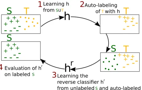
A crucial question in domain adaptation is the validation of the hyperparameters. One solution is to follow the principle proposed by Zhong et al. (2010) which relies on the use of a reverse validation approach. This approach is based on a so-called reverse classifier evaluated on the source domain. We propose to follow it for tuning the parameters of PBDA, DASVM and CODA. Note that Bruzzone and Marconcini (2010) have proposed a similar method, called circular validation, in the context ofDASVM.

Concretely, in our setting, givenk-folds on the source labeled sample (S =S1∪. . .∪Sk), k-folds on

the unlabeled targetT sample (T =T1∪. . .∪Tk) and a learning algorithm (parametrized by a fixed tuple

of hyperparameters), the reverse cross validation risk on the ith _{fold is computed as follows. Firstly, the}

source set S\Si is used as a labeled sample and the target setT \Ti is used as an unlabeled sample for

learning a classifier h0. Secondly, using the same algorithm, a reverse classifier h0r _{is learned using the}

self-labeled sample{(x, h0(x))}x∈T\Ti as the source set and the unlabeled part ofS\Si as target sample. Finally, the reverse classifierh0r_{is evaluated onS}

i. We summarize this principle on Figure2. The process

is repeatedktimes to obtain the reverse cross validation risk averaged across all folds.

6.3

Toy Problem: Two Inter-Twinning Moons

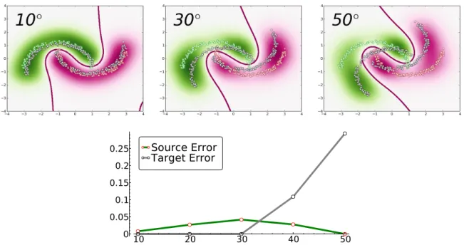
The source domain considered here is the classical binary problem with two inter-twinning moons, each class corresponding to one moon (Figure3). We then consider seven different target domains by rotating anticlockwise the source domain according to seven angles (from 10◦ to 90◦). The higher the angle, the more difficult the problem becomes. For each domain, we generate 300 instances (150 of each class). More-over, to assess the generalization ability of our approach, we evaluate each algorithm on an independent test set of 1,000 target points (not provided to the algorithms). We make use of a Gaussian kernel for all the methods. Each domain adaptation problem is repeated ten times, and we report the average error rates on Table1. Note that sinceCODAdecomposes features for applying co-training, it is not appropriate here (we have only two features).

We remark that our PBDA provides the best performances except for 50◦ and 20◦, indicating that PBDAaccurately tackles domain adaptation tasks. It shows a nice adaptation ability, especially for the hardest problem, probably due to the fact that disρ is tighter and seems to be a good regularizer in a

domain adaptation situation. The adaptation versus risk minimization trade-off suggested by Theorem12

10_{We made our code available at the following URL:http://graal.ift.ulaval.ca/pbda/} 11_{Available athttp://www.scipy.org/}

++++

+

h

r

h

1

2

Auto-labeling

of with h

3

Learning the

reverse classi

fi

er h

from unlabeled and auto-labeled

SUT _T S T r

4

Evaluation of h

on labeled

+ +

+

+

+

--

-

-

-S

T

T

-- -

-

-S

+ +

+

+

+

--

-

-

-Learning h

from

S

++++

+

T

-- -

-

-Figure 2: The principle of the reverse/circular validation in our setting.

Table 1: Average error rate results for seven rotation angles. PBGD3CV SVMCV DASVMRCV PBDARCV 10◦ 0 0 0 0 20◦ 0.088 0.104 0 0.094 30◦ 0.210 0.24 0.259 0.103 40◦ 0.273 0.312 0.284 0.225 50◦ 0.399 0.4 0.334 0.412 70◦ 0.776 0.764 0.747 0.626 90◦ 0.824 0.828 0.82 0.687

appears in Figure 3. Indeed, the plot illustrates thatPBDA accepts to have a lower source accuracy to maintain its performance on the target domain, at least when the source and the target domains are not so different. Note, however, that for large angles, PBDAprefers to “focus” on the source accuracy. We claim that this is a reasonable behavior for a domain adaptation algorithm.

6.4

Sentiment Analysis Dataset

We consider the popularAmazon reviewsdataset (Blitzer et al.,2006) composed of reviews of four types of Amazon.comc products (books, DVDs, electronics, kitchen appliances). Originally, the reviews cor-responded to a rate between one and five stars and the feature space (of unigrams and bigrams) has on average a dimension of 100,000. For sake of simplicity and for considering a binary classification task, we propose to follow a setting similar to the one proposed byChen et al.(2011). Then the two possible classes are: +1 for the products with a rank higher than 3 stars,−1 for those with a rank lower or equal to 3 stars. The dimensionality is reduced in the following way: Chen et al.(2011) only kept the features that appear at least ten times in a particular DA task (it remains about 40,000 features), and pre-processed the data with a standard tf-idf re-weighting. One type of product is a domain, then we perform twelve domain adaptation tasks. For example, “books→DVDs” corresponds to the task for which books is the source domain and DVDs the target one. The algorithms use a linear kernel and consider 2,000 labeled source examples and 2,000 unlabeled target examples. We evaluate them on separate target test sets proposed by Chen et al.(2011) (between 3,000 and 6,000 examples), and we report the results on Table 2. We make the following observations.

First, as expected, the domain adaptation approaches provide the best average results. Then,PBDA is on average better than CODA, but less accurate than DASVM. However, PBDA is competitive: the results are not significantly different fromCODAandDASVM. Moreover, we have observed thatPBDAis significantly faster thanCODAandDASVM: these two algorithms are based on costly iterative procedures increasing the running time by at least a factor of five in comparison ofPBDA. In fact, the clear advantage ofPBDAis that we jointly optimize the terms of our bound in one step.

Figure 3: Illustration of the decision boundary of PBDAon three rotations angles for fixed parameters

A = C = 1. The two classes of the source sample are green and pink, and target (unlabeled) sample is gray. The bottom plot shows corresponding source and target errors. We intentionally avoid tuning PBDA parameters to highlight its inherent adaptation behavior.

6.5

Combining

and Representation Learning

As discussed in the introduction, there exist several families of approaches used to tackle the domain adaptation problem. The present work focuses on the minimization of a distance metric between the source and target distributions. Now, we ask ourselves whether it can be fruitful to combine our PBDA algorithm with another approach. To do so, we executed PBDA on top of the Marginalized Stacked Denoising Autoencoders (mSDA) introduced byChen et al.(2012).

In brief,mSDAis an unsupervised algorithm that learns a new representation of the training samples. As a “denoising autoencoders” algorithm, it finds a representation from which one can (approximately) reconstruct the original features of an example from its noisy counterpart. The originality of mSDAis to learn a representation that allows reconstructing both source and target unlabeled examples. Then, one can execute any supervised learning algorithm on the new representation of source samples, for which the labels are known.

That is, given a source sample S = {(xs_i, ys_i)}m

i=1 and a target sampleT = {(x

t i)}

m0

i=1, mSDA takes

the unlabeled parts ofS and T, {xs₁, . . . ,xs_m,xt₁, . . . ,xt_m0}, and learn a feature mapf :X →X0, where

X0 is a new input space (of real-valued vector). In (Chen et al., 2012), a linear SVMis executed using

Sf ={(f(xsi), y s i)}

m

i=1as training data, and the hyper-parameterCis selected by standard cross-validation.

We compare the performance ofSVMonmSDArepresentation toPBDAon the same representations. That is, we obtain a new representation of both sourceSf ={(f(xsi), ysi)}mi=1and targetTf={(f(xti))}m

0 i=1

data, usingmSDA. Then, we executePBDAusingSf andTf.

This comparison is done using theAmazon reviewsdataset. For the sake of comparison, we used the dataset pre-processed byChen et al. (2012), which is slightly different from the one used in Section6.4. Indeed, each domain share the same 5,000 features, and no tf-idf re-weighting is applied. For each pair source-target,mSDArepresentations are generated using acorruption probability of 50% and anumber of layers of 5. Then, SVMandPBDAare executed on the same representations.

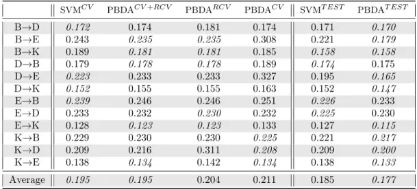
The results are reported in Table 3. The PBDA algorithm, when we select the hyperparameter by reverse cross-validation (PBDARCV), is not always as good as the cross-validated SVM (SVMCV). However, by looking closer at the results, we notice that there often exists hyperparameters for whichPBDAis better on the testing set than the best achievableSVM(as reported by the columnsPBDAT EST andSVMT EST). This suggests that it might be advantageous to mix mSDAand PBDAlearning strategies. However, the hyperparameters selection is still a challenge in domain adaptation, when we do not have any target labels, even if the reverse cross-validation method is a sound strategy. For exploratory purposes, we report on Table3the risk ofPBDAwhile performing the model selection by standard cross-validation (PBDACV) and

Table 2: Error rates for sentiment analysis dataset. B, D, E, K respectively denotes books, DVDs, electronics, kitchen.

PBGD3CV SVMCV DASVMRCV CODARCV PBDARCV B→D 0.174 0.179 0.193 0.181 0.183 B→E 0.275 0.290 0.226 0.232 0.263 B→K 0.236 0.251 0.179 0.215 0.229 D→B 0.192 0.203 0.202 0.217 0.197 D→E 0.256 0.269 0.186 0.214 0.241 D→K 0.211 0.232 0.183 0.181 0.186 E→B 0.268 0.287 0.305 0.275 0.232 E→D 0.245 0.267 0.214 0.239 0.221 E→K 0.127 0.129 0.149 0.134 0.141 K→B 0.255 0.267 0.259 0.247 0.247 K→D 0.244 0.253 0.198 0.238 0.233 K→E 0.235 0.149 0.157 0.153 0.129 Average 0.226 0.231 0.204 0.210 0.208

Table 3: Error rates formSDArepresentations on sentiment analysis dataset. SVMCV PBDACV+RCV PBDARCV PBDACV SVMT EST PBDAT EST

B→D 0.172 0.174 0.181 0.174 0.171 0.170 B→E 0.243 0.235 0.235 0.308 0.221 0.179 B→K 0.189 0.181 0.181 0.185 0.158 0.158 D→B 0.179 0.178 0.178 0.189 0.174 0.175 D→E 0.223 0.233 0.233 0.327 0.195 0.165 D→K 0.152 0.155 0.155 0.163 0.152 0.147 E→B 0.239 0.246 0.246 0.251 0.226 0.233 E→D 0.233 0.232 0.230 0.232 0.225 0.230 E→K 0.128 0.123 0.123 0.133 0.127 0.115 K→B 0.229 0.230 0.230 0.225 0.221 0.217 K→D 0.209 0.216 0.311 0.208 0.209 0.200 K→E 0.138 0.134 0.142 0.134 0.138 0.133 Average 0.195 0.195 0.204 0.211 0.185 0.177

while we consider the mean of the cross-validation and the reverse cross-validation score (PBDACV+RCV). Interestingly, the latter method is a better selection criterion than taking one or the other validation risk separately in this experiment, both being misleading in some situations.12

7

Generalization of the PAC-Bayesian Domain Adaptation

The-orems to Multisource Domain Adaptation

In this section, we generalize our main analysis to multisource domain adaptation.

7.1

Multisource Domain Adaptation Setting

We now consider ndifferent source domains {PSj}

n

j=1 over X×Y (along with{DSj}

n

j=1 the associated

marginal distributions overX). In addition to the targetm0-sampleT withm0 unlabeled examples drawn

i.i.d. from the target marginalDT, we have onei.i.d. source learning sampleSjper domainsPSj (possibly of different sizes).

Similarly toBen-David et al. (2010a), we study this issue when the relationship between the source domains and the target one is captured by a distributionv over the set of source domains{PSj}

n

j=1. This

12_{It is important to point out that experiments on other datasets showed us that theCV+RCV method does not}

distribution defines a mixture of source domains that we denote byPv

S, and its marginal over X byDvS,

andSv_={S

j}nj=1corresponds to the set of source samples. On the source domains, we then consider the

followingv-weighted true error of the Gibbs classifierGρ:

RPv S(Gρ) def = E P_Sj∼vRPSj(Gρ) = E P_Sj∼vhE∼ρRPSj(h) = n X j=1 v(PSj) E h∼ρRPSj(h).

Its empirical counterpart is defined as

RSv(Gρ) def = n X j=1 v(PSj)E h∼ρRSj(h).

Note that another solution for tackling multisource domain adaptation in a PAC-Bayesian philosophy could be to learn different posterior distribution overHfrom different sources. Indeed, instead of learning a shared ρon every domain (including the target one), we can learn a model for each domain, and then try to learn a good target majority vote over this set of models. In this situation, one could derive a PAC-Bayesian analysis similar to the one provided byPentina and Lampert (2014) for life-long learning. However, this setting clearly appears to be not pertinent to extend our one-source domain analysis to multiple sources, since they treat the prior distribution as a random variable, which is not our setting.

7.2

Generalization of the

ρ

-Disagreement to Multiple Sources

One natural solution to generalize theρ-disagreement of Definition1 to the multisource setting described in above is to make use of thev-weighted sum of eachρ-disagreement between a source distribution and the target oneED_Sj∼v disρ(DSj, DT), for which we can easily extend Theorem9. However, we prefer to consider the following definition that is clearly tighter than the latter one.

Definition 2. Let H be a hypothesis class. For marginal distributions {DSj}

n

j=1 and DT over X, any

distributionv on {DSj}

n

j=1, any distribution ρonH, the domain disagreementdisρ(DvS, DT)between the

mixture of source distribution Dv

S and the target distributionDT is defined by

disρ(DvS, DT) def = E (h,h0_)∼ρ2 RDT(h, h 0_{)− E} D_Sj∼v RDSj(h, h 0₎ = RDT(Gρ, Gρ)−_DE Sj∼v RD_Sj(Gρ, Gρ) .

As noticed before, we trivially have

disρ(DSv, DT) ≤ E

D_Sj∼v disρ(DSj, DT). (16)

Therefore, one can use the various PAC-Bayesian bounds presented in Section 4.1.3 to obtain an empirical guarantee over disρ(DSv, DT) from a collection of observations from each domain. In particular,

Corollary2 below is directly obtained from Theorem7.

For sake of simplicity, the results presented for the multisource setting suppose that every sample shares the same sizem. We use the shortcut notation Sv _∼(Pv

S)m to denote the collection of n source

samples ofmexamples. That is,Sv_={S

j}nj=1, whereSj ∼(PSj)

m_.

Corollary 2. For any distributions{DSj}

n

j=1 andDT overX, any set of hypothesesH, any distribution

v over {DSj}

n

j=1, any prior distribution π over H, any δ ∈ (0,1], and any real number α > 0, with a

probability at least1−δover the choice of Sv_∼(Pv

S)m andT ∼(DT)m, for everyρonH, we have

disρ(DSv, DT) ≤ 2α 1−e−2α " E D_Sj∼v disρ(S v , T) +2 KL(ρkπ) + ln 2 δ + lnn m×α + 1 # −1.

Proof. We upper bound the right-hand side of Equation (16) by upper-bounding each individual term of the expectation using Theorem7. That is, we bound

v(PS1) disρ(S1, T), v(PS2) disρ(S2, T), . . . , v(PSn) disρ(Sn, T), each one with probability 1−δ

n. Thereafter, we regroup thesenbounds together to obtain the final result,

which stands with probability 1−δ.

The bound given by Corollary2can suffer from the inequality of Equation (16). A better generalization guarantee is given by Theorem 13below that bounds directly disρ(DvS, DT), and does not rely on a term

“lnn” like we have in Corollary2.

Theorem 13. For any distributions{DSj}

n

j=1 andDT overX, any set of hypothesesH, any distribution

v over {DSj}

n

j=1, any prior distribution π over H, any δ ∈ (0,1], and any real number α > 0, with a

probability at least1−δover the choice of Sv_∼(Pv S)

m _{andT ∼(D}

T)m, for everyρonH, we have

disρ(DSv, DT) ≤ 2α 1−e−2α disρ(Sv, T) + 2 KL(ρkπ) + ln2_δ m×α + 1 −1.

Proof. Deferred to AppendixE.

Note that Theorem 6, Corollary 1 and Theorem 8 can also be rewritten to bound the multisource domain disagreement following the same proof techniques as we used for Theorem13.

7.3

Multisource Domain Adaptation Bound for the Stochastic Gibbs

Classi-fier

Let now generalize the domain adaptation bound ofRPT(Gρ) presented by Theorem9to our multisource setting.

Theorem 14. LetHbe a hypothesis class. We have

∀ρon H, ∀v on{PSj} n j=1, RPT(Gρ) ≤ RPSv(Gρ) + 1 2disρ(D v S, DT) +λvρ,

whereλvρis the deviation between the expected joint error ofGρ on the source domains and the target one:

λv_ρ def= E (h,h0_)∼ρ2 " E (x,y)∼PT L_0-1 h(x), y L_0-1 h0(x), y − E P_Sj∼v (x,yE)∼P_SjL0-1 h(x), y L_0-1 h0(x), y # = ePT(Gρ, Gρ)− E P_Sj∼vePSj(Gρ, Gρ) . (17)

See Equation (6) for the definition ofeP_Sj(Gρ, Gρ).

Proof. We follow the same steps as in the proof of Theorem9. Indeed, from Equation (12), we have

RPT(Gρ)−RPSv(Gρ) = 1 2 RDT(Gρ, Gρ)− E P_Sj∼vRDSj(Gρ, Gρ) +ePT(Gρ, Gρ)− E P_Sj∼vePSj(Gρ, Gρ) ≤ 1 2 RDT(Gρ, Gρ)− E P_Sj∼vRDSj(Gρ, Gρ) + ePT(Gρ, Gρ)− E P_Sj∼vePSj(Gρ, Gρ) = 1 2disρ(D v S, DT) +λvρ.

7.4

PAC-Bayesian Theorem for Multisource Domain Adaptation

Building on Theorems13and14, we now present a PAC-Bayesian theorem for multisource domain adap-tation.

Theorem 15. For any domains {PSj}

n

j=1 and PT (respectively with marginals {DS}nj=1 and DT) over

X×Y, any distribution v over{PSj}

n

j=1, and for any setH of hypotheses, for any prior distribution π

over H, any δ∈(0,1], with a probability at least 1−δ over the choice of Sv ∼(P_Sv)m andT ∼(DT)m,

for every ρoverH, we have

RPT(Gρ) ≤ c 0_R Sv(G_ρ) +α01 2disρ(S v_{, T) + c}0 c + α0 α _{KL(ρkπ) + ln}3 δ m +λ v ρ+12(α 0_−1),

whereλv_ρ is defined by Equation (17), and wherec0 def= c

1−e−c and α

0def

= 2α 1−e−2α.

Proof. In Theorem14, replaceRSv(G_ρ) and dis_ρ(Dv_S, D_T) by their upper bound, obtained from Theorem5 and Theorem13, withδ chosen respectively as δ₃ and 2₃δ.

Theorem15above is a generalization of Theorem11. It is straightforward to generalize Theorems10 and12as well to the multisource setting.

It is important to point out that the above theorem, which naturally generalizes our one-source domain analysis, supposes that the distributionvoverPv

Sis fixed (or known). However, we can prove generalization

bounds that involve v given a prior distribution uover Pv

S. On the one hand, it is possible to derive a

result for a distributionρonHfixed. On the other hand, such a result can be also derive onv and ρat the same time. These two results can be helpful to derive another kind of approach, and we detail and discuss these bounds in the in Section8.1.

7.5

for Multisource Domain Adaptation

Regarding the results of Section7, optimizing the PAC-Bayesian multisource domain adaptation bounds of Theorem15is equivalent to minimize the following trade-off

C m RSv(G_ρw) +A mdis_ρw(Sv, T) + KL(ρ_wkπ₀), where disρw(S v_{, T) =} RSv(Gρw, Gρw)−RT(Gρw, Gρw) , and Sv _{= {S} j}nj=1 = {(xs

ij, yijs}mi=1 _j=1 are the n source samples coming from the mixture of source

domainsPv

S, andT ={(xti)}im=1 is the target sample. Given the vectors of weightsv={v(PSj)}

n j=1 over

the source domains, finding the optimalρw is then equivalent to find the vectorw that minimizes

C n X j=1 m X i=1 v(PSj) Φ y