DTMC: An Actionable e-Customer Lifetime Value Model
Based on Markov Chains and Decision Trees
Peter Paauwe
Econometric Institute Erasmus University P.O. Box 1738 3000 DR, Rotterdam The NetherlandsPeter van der Putten
∗LIACS Leiden University
P.O. Box 9512 2300 RA, Leiden, The
Netherlands
Michiel van Wezel
†Econometric Institute Erasmus University P.O. Box 1738 3000 DR, Rotterdam The Netherlands
[email protected]
ABSTRACT
We describe a model for estimating the customer lifetime value (CLV) of customers in an e-commerce environment. The model is explained and experiments are performed on real-life data from a large Dutch Internet retailer.
Our method results in CLV estimates that have similar ac-curacy to estimates generated by the commonly used model, while keeping the number of customer segments much lower, and thus more ‘actionable’.
Categories and Subject Descriptors
H.4.m [Information Systems Applications]: Miscella-neous; I.2.6 [Artificial Intelligence]: Learning
Keywords
Customer Lifetime Value, E-Commerce, CART, Marketing, Markov Chains
General Terms
Algorithms, Economics, Management
1.
INTRODUCTION
E-commerce sales have exhibited a staggering growth in the last few years. The U.S. Census Bureau [13] estimates that total retail e-commerce sales in the third quarter of 2006 increased 21% with respect to the same period in 2005, whereas total retail sales increased only 5%. The sales vol-umes for online retail was$27.5 billion in this period, corre-sponding to 2.8 percent of the total sales volume of$991.7 billion. Other sources show similar growth percentages [12]. It is thus clear that the web is becoming an increasingly
∗Also at Chordiant software. †Corresponding author
Permission to make digital or hard copies of all or part of this work for personal or classroom use is granted without fee provided that copies are not made or distributed for profit or commercial advantage and that copies bear this notice and the full citation on the first page. To copy otherwise, to republish, to post on servers or to redistribute to lists, requires prior specific permission and/or a fee.
ICEC’07, August 19–22, 2007, Minneapolis, Minnesota, USA. Copyright 2007 ACM 978-1-59593-700-1/07/0008 ...$5.00.
important sales channel and companies should strive for a successful web site.
Various metrics for measuring web site success have been proposed in the literature. (See, e.g., [10, 5].) Commonly used metrics for success include traffic count, conversion rate, click through ratio, user satisfaction, frequency of use and likelihood of return. Only recently [4], there has been some interest in the e-Commerce community in the use of
Customer Lifetime Value (CLV) as a basis for measuring web site success. Briefly, the CLV of a customer is the ex-pected value of the (discounted) profit she will generate now and in the future. Thus, contrary to the previous metrics, CLV takes a ‘long term approach’. The sum of the CLV’s for all customers is often referred to acustomer equity(CE). The CLV concept is adopted from traditional marketing lit-erature [3].
There are two motivations for using CLV/CE as a metric for web site success. First the CLV metric can be used to guide marketing efforts and make these more accountable, including data-mining efforts to promote sales, and help in establishing a firm long-term relationship with high-value customers. Second, CE can play a role in establishing the value of an e-commerce firm [11, 8].
Berger and Nasr [1] proposed a series of mathematical models for calculating CLV in different scenarios, whereas much of the earlier literature had been – in their words – ‘dedicated to extolling its use as a decision criterion’. These models were subsequently re-formulated and unified by cast-ing them into a Markov chain framework by Pfeifer and Car-raway. Unlike cross sectional or basic longitudinal models for predicting CLV, Markov chains can be used to explicitly model the dynamics of how CLV develops over time for a given customer. Details on this latter model will be given in Section 2.
Contrary to many traditional marketing environments, e-commerce environments are typically very data-rich. Unfor-tunately, the traditional Markov based model from reference [6] is unable to cope with this data-richness, because the ex-istence of large numbers of attributes and with numerical attributes leads to an explosion of the number of states in the Markov chain and/or partitioning problems.
In this paper, we propose a two-stage CLV model, called DTMC, that is based on CART. The addition of the de-cision tree (CART) step enables us to apply the Markov chain framework to with data-rich environments by group-ing the customers into segments of similar value based on
their attributes, thereby reducing the number of states. Be-sides enabling the Markov approach for e-commerce data, this has the added advantage that the model becomes more actionable, since it is easier to direct a single effort to a com-plete segment than varying efforts to each customer. Details on the DTMC model will be given in Section 3.
We evaluated the DTMC model using real world customer purchase data from a large Dutch Internet retailer selling ink cartridges for ink-jet printers. This gives encouraging results. These experiments and results are described in Sec-tions 4 and 5 respectively. Finally, Section 6 gives conclu-sions, discussion and an outlook.
2.
CUSTOMER EQUITY AND CUSTOMER
LIFETIME VALUE
This section gives an overview of CLV and the model from [6] to estimate it.
Customers are seen as an asset in customer centric market-ing, therefore financial theory is very useful when estimating CLV. The value of an asset is measured by discounting its future value to the present, thus a basic CLV model can be formulated as CLVi= T X t=1 Profiti,t (1 +d)t, (1)
whereCLVi refers to lifetime value of customeri,T is the time horizon,P rof iti,tis the profit gained from customeri
at timet and d is the discounting factor. Profit is gained when revenues are larger then associated costs. Consequently, the CLV model can be split into two parts. Mathematically this becomes CLVi= T X t=1 Revenuei,t (1 +d)t − T X t=1 Costi,t (1 +d)t. (2)
Because customer relationships are viewed as an asset. The total value of all customer relationships can be seen as an equity to the firm. Thus the sum of all individual CLV’s of customers in the industry results in customer equity (CE):
CE=
I
X
i=1
CLVi. (3)
The CLV model of Equation 2 is all that is needed to calcu-late CLV. The discount factor can be easily determined from business rules, but estimating future revenues and costs for every customer is were the difficulty lies.
Different approaches to this problem can be found in liter-ature. For instance, references [9] and [14] develop individ-ual level CLV models based on marketing theory, whereas [7] proposes a segment level CLV model based on pre-determined segments. As stated earlier, in this paper we build on the Markov chain approach from [6].
Pfeifer and Carraway propose the use of RFM variables, i.e. variables capturing the recency (time elapsed since the last purchase), frequency (total number of purchases) and monetary value (total generated income) of a customer. Af-ter discretization, these variables are used to define the states in the Markov model. We now give a short example, adopted from [6], to illustrate this idea.
The example uses only recency to model customer be-havior, which is recorded months. The different values for recency are then used as states for the Markov chain. In
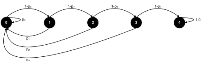
1 2 3 4 1.0 1-p0 0 p0 1-p1 p1 p2 p3 1-p2 1-p3
Figure 1: Graphical representation of the switching probabilities in the Markov matrix.
the example 5 states are defined. State 0 corresponds to re-cency 0, indicating a purchase in the current period. States 1, 2, and 3 respectively correspond to recency 1, 2, and 3 indicating a purchase 1, 2, or 3 periods ago. And state 4 corresponds to recency 4 or more. A customer in state 4 is considered to be a lost customer and state 4 therefore is said to be a ’dead state’, since its not possible to return to another state from this state.
These states are then used to construct a Markov matrix
P, where element Pij represents the probability of going
from stateito statej. This matrix can either be estimated by experts or by using historical data. Figure 1 gives a graphical representation of such a matrix. (This figure was adopted from [6].) Each node in the figure represents a state and each arrow a possible switch with its associated probability.
Each customer arriving in a state represents a certain value for the company. A reward vector is therefore used to assign a value to each state. This is done by including gains and costs. N C is used to present the net contribution of a state and M indicates the marketing expenses. Gains are only being made if a customer purchases anything and therefore only state 0 has a net contribution. Marketing ex-penses are made if a customer is thought of as active. Thus there are no marketing expenses for state 4. This results in the following reward vector
R= 2 6 6 6 4 N C−M −M −M −M 0 3 7 7 7 5 .
Now by combining the Markov matrix and reward vector the CLV of a customer in stateswith recencyrcan be val-uedT periods ahead. Therefore the transition probabilities have to be calculated for every future periodt(t= 1, . . . , T). These probabilities are found by multiplying the Markov matrix ttimes, which is a well known property of Markov chains [6]. Thus for every periodta transition matrixPt is
found. This matrix has to multiplied by the reward vector for every period, which results in the value derived from a customer in that period. By summing over all periods CLV is found: CLV= T X t=0 [(1 +d)−1P]tR. (4) This equation shows how the vector CLV is calculated using a Markov chain. This vector contains the expected future value, T periods ahead, of a customer in state s
(s = 1, . . . , S) at time t = 0. Furthermore d is the dis-count rate of money, P is the Markov matrix containing
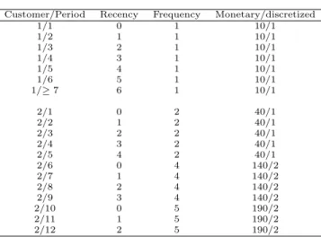
Customer/Period Recency Frequency Monetary/discretized 1/1 0 1 10/1 1/2 1 1 10/1 1/3 2 1 10/1 1/4 3 1 10/1 1/5 4 1 10/1 1/6 5 1 10/1 1/≥7 6 1 10/1 2/1 0 2 40/1 2/2 1 2 40/1 2/3 2 2 40/1 2/4 3 2 40/1 2/5 4 2 40/1 2/6 0 4 140/2 2/7 1 4 140/2 2/8 2 4 140/2 2/9 3 4 140/2 2/10 0 5 190/2 2/11 1 5 190/2 2/12 2 5 190/2
Table 1: Typical discretized data for the e-CLV model. Recency is recorded in months with a max-imum of 6. Frequency represents the aggregated number of purchases, and has a maximum of 6, and Monetary value is the aggregated spending for that customer. Monetary is discretized by introducing categories of 100 dollars wide. (Monetary 1 rep-resents spending between$0 and $100, 2 represents spending between$100and $200, and so on.)
switching probabilities between states andRis the reward vector containing the monetary contribution of each state.
Now, by counting the number of customers in each state att= 0 customer equity can be calculated. This is done by multiplying this number by the respective CLV, as shown below. CE= S X s=1 CLVsCs (5)
In above equationCLVs is the CLV of a customer in state
s andCs is the number of customers in this state at time
t= 0.
The paper by Pfeifer and Carraway is mostly intended to show the usefulness of Markov chains in CLV modeling, while no empirical use of their model is presented. This gap is filled by the e-CLV model proposed by Etzion et. al. [4], which is based on attributes specific to the e-commerce domain. In their application to online electronic auctions, Etzion et. al. use customer sessions, bids, and purchases to derive various attributes, such as recency and frequency of sessions, bids, and purchases.
After discretization, these attributes are used to form the states of the Markov matrix, i.e., every possible combination of discretized values for these attributes forms a separate state. An example of such discretized data is shown in Ta-ble 1. The Markov matrixPis then estimated by counting the state transitions customers go through in these data. A major drawback is that the number of states grows exponen-tially with the number of attributes: The example generates 7.5.2 = 70 states.
The Markov model based on RFM variables seems a good solution to estimate CLV for Internet retailing businesses, simply because complete customer purchase records to ex-tract RFM variables are always available since purchases have to be billed and/or shipped to customers. Secondly
other information, for instance site visiting behavior may be available, which can be used for prediction. The study by [4] already uses such information.
Although conceptually elegant, the model put forward by [6] is susceptible to some criticism. A first point of critique is the so called ’dead state’. If customers are inactive for a certain number of periods they are considered lost for good. And, if they return to the company they are treated as new customers. [8] indicate that this approach systematically underestimates CLV. In [14] this problem is also put forward. With Markov chains this problem is easily solved by letting the possibility exist to return to other states from the ’dead state’.
Secondly, the exponential number of states leads to prob-lems. The first problem is that the reward vector is difficult to estimate since many of the states may lack observations. (Therefore, the authors of [6] suggest it should be estimated by experts, but this may be infeasible or give unreliable esti-mates.) Moreover, it is important for business managers to keep the states actionable, since marketing strategies will be based on different CLV’s. Designing 70 different strategies, as in the example dataset, is unfeasible.
Therefore a segment based approach as in [7] may be more practical. Their approach is inappropriate for our purposes however, since it is tailored to the telecommunications in-dustry, where customers have long term contracts, lending itself to survival modeling. In our case, these long term contracts are lacking, and a Markov model approach seems more appropriate, but states should somehow be grouped into distinctive clusters in order to keep them actionable. The next section will introduce such a model.
3.
DTMC MODEL
This section will introduce the Decision Tree Markov Chain (DTMC) model, able to estimate segment level CLV. The next section will illustrate the use of the DTMC model by presenting a real life business case. To estimate segment level CLV a CART decision tree [2] is used to form dis-tinctive groups based on the input variables. The groups formed by the CART tree are subsequently used as states in the Markov chain model.
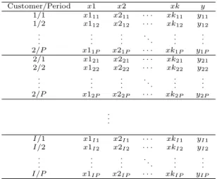
Data for the DTMC model has to consist of variables de-scribing customers. These variables have to be recorded for a number of periods. The reward generated by a customer also needs to be recorded every period. This typical data layout is shown in Table 2. For every customer (1 toI) for every period (1 to P) descriptive variables x1, . . . , xk and reward/spendingyare recorded.
Various descriptive variables can be used for the segmen-tation. for instance demographic information, the number of site visits this period, or RFM variables as in [6] and [4]. Traditional RFM variables are aggregated over the com-plete customer history. Since we want to find segments of customers with similar valuewithin one periodrather than over their entire lifespan for use in the Markov model, we use
per periodversions of the RFM variables in the experiments below. Recency now indicates how many periods ago a cus-tomer bought something relative to this period, frequency is the number of purchases during this period and monetary is the total amount spent during the current period.
The choice for per-period-RFM variables introduces a prob-lem, since CART will place all customers who have been in-active for at least one period in the same state. This way
Customer/Period x1 x2 xk y 1/1 x111 x211 · · · xk11 y11 1/2 x112 x212 · · · xk12 y12 . . . . . . . . . . .. . . . . . . 2/P x11P x21P · · · xk1P y1P 2/1 x121 x221 · · · xk21 y21 2/2 x122 x222 · · · xk22 y22 . . . . . . . . . . .. . . . . . . 2/P x12P x22P · · · xk2P y2P . . . I/1 x1I1 x2I1 · · · xkI1 yI1 I/2 x1I2 x2I2 · · · xkI2 yI2 . . . . . . . . . . .. . . . . . . I/P x1IP x2IP · · · xkIP yIP Table 2: Typical data for the DTMC model.
valuable customer discrimination information is lost. This problem is circumvented by deleting the records that con-tain no actual purchases. Only data concon-taining purchases is then used to fit the CART tree. Such data is illustrated in Table 3.
Record Customer/Period Recency Frequency Monetary
1 1/1 0 1 10 2 2/1 0 2 40 3 2/6 5 2 100 4 2/10 4 1 50 5 3/6 0 3 75 6 4/3 0 4 125 7 4/11 8 4 150 8 4/14 3 5 250 9 4/16 2 2 75
Table 3: Typical RFM data for the DTMC model, with non-buy periods left out.
Using a CART tree, the monetary amount is estimated using only recency and frequency. This groups the data into certain value segments, through the leafs found at the bot-tom of the tree. Besides the states defined by the CART tree we introduced an ‘end state’, which customers enter if they have been inactive for 6 periods. These customers are considered lost, or semi-lost for the company. (We will dis-cuss this shortly.) Figure 2 depicts the process of assigning states to records. States 1 through 4 represent the ‘buy’ states modeled by the CART tree, state 5 represents the end state. As an example: leaf 2 of the CART tree takes records 3,4 and 9, from Table 3 and thus has an average value of $75.
One might wonder why we did not use the actual value segments as states for the Markov model, i.e., create a seg-mentation based on the Monetary attribute and discard the Recency and Frequency attributes. However, there is a large random component in short term customer buying behavior which would lead to quite random transition behavior across states, causing an explosion of uncertainty with even a low number of iterations.
Expected value is a better reflection of the potential value of a customer than actual value, and will lead to more stable state switching behavior. Accordingly, our approach seg-ments customers based on a limited set of non monetary attributes that are assumed to have a relation to future
buy-begin 1 2 3 4 5 begin 0 2 0 2 0 0 1 0 0 1 0 0 1 2 0 0 1 0 0 1 3 0 0 0 0 0 2 4 0 0 1 0 1 0 5 0 0 0 0 1 0
Figure 3: The number of state transitions counted from Table 3. The row represents the old state, the column the new state.
ing behavior. In this study we used the classical attributes recency and frequency, but in principle any combination of suitable attributes can be used.
After the CART step, the states of the Markov matrix are known. The states for the example are summarized in Table 4. The average contribution of each state is also shown in this table. Together these contributions form the reward vector needed to calculate CLV. Table 4 also introduces a begin state, which capturespotentialcustomers. Transition probabilities from this state to the other states indicate how likely it is that a new customer will enter in a certain state.
Frequency Recency State Contribution
- - begin 0 ≤2 0 1 25 ≤2 ≥1 2 75 >2 0 3 100 >2 ≥1 4 200 0 6 5 0
Table 4: State definitions for the Markov matrix.
There are two interpretations we can give to state 5, the end state. Customers arriving in state 5 can be considered lost for good, which makes returning to one of the other states impossible. This approach is followed by [6] and [4]. But, customers can also be considered to be semi-lost. This way it is possible to return to the other states. Note the introduction of this semi-lost concept is also a contribution of this paper
Both scenarios will be tested with our empirical applica-tion presented in the remainder.
The state sequence of every customer is used to calculate the switching probabilities between states. This is done by a similar procedure as in [4]. First the Markov matrix is initialized to zero. Then the state transitions are counted. The results of this counting procedure applied to the data of Table 3 is shown in Figure 3. (The transitions to state 5 are not shown in Table 3 but are inferred from the original data.) We then transform this matrix into a Markov matrix by normalizing each row (except the row representing the end state) to 1. If we want to use the ‘lost-for-good’ scenario we first set all counts from the ‘semi-lost-state’ (state 5) to other than the end states to 0, thereby ignoring such transitions had they occurred. (In the example such a transition occurs from state 5 to state 4.) Depending which procedure we apply we end up with one of the matrices in Figure 4.
The last modeling step is the estimation of average CLV per state T periods ahead. In principle, this is done using Equation 4, but since we discarded observations where no purchase was made we must make a few adjustments. First, we compute the average between-purchase-period by divid-ing the length of the total lifespan for each customer by the number of occasions in which she made a purchase and
de-1 2 3 4 Purchase record? (Frequency>0) 5 State Frequency=0, Recency=6? Yes No Discard record Yes No $150 $50 State State State State $25 $75 $100 $200 Frequency <=2 Frequency > 2
Recency=0 Recency>=1 Recency=0 Recency>=1 $100
Use CART model
Figure 2: Assigning states to records. The encircled numbers represent the states.
begin 1 2 3 4 5 begin 0 0.5 0 0.5 0 0 1 0 0 0.5 0 0 0.5 2 0 0 0.5 0 0 0.5 3 0 0 0 0 0 1 4 0 0 0.5 0 0.5 0 5 0 0 0 0 0.25 0.75 begin 1 2 3 4 5 begin 0 0.5 0 0.5 0 0 1 0 0 0.5 0 0 0.5 2 0 0 0.5 0 0 0.5 3 0 0 0 0 0 1 4 0 0 0.5 0 0.5 0 5 0 0 0 0 0 1
Figure 4: Markov matrices for semi-lost scenario (top) and lost-for-good scenario (bottom).
note the result byN. (Thus,N= 2.7 means that on average there is a 2.7 month period between purchases.) Next, we redefine the total number of periodsT to reflect the longer period lengthTnew=dT /Ne, and we accordingly adjust the
discount ratednew = (1 +d)T /N−1.
This results in the following CLV equation:
CLV= Tnew X t=1 ((1 +dnew) −1 M)tR, (6)
whereCLVis theS×1 vector containing the average CLV for every states(s= 1, . . . , S),Mis the Markov transition matrix containing the switching probabilities, dnew is the
discounting factor and R is the reward vector containing the estimated expenditure of a customer when he arrives in a certain state. In practice the final term of this sum may not represent a fullN-month period and should be weighted accordingly.
Table 5 shows the resulting CLV’s for the lost for good and semi-lost scenarios. For each state, the number of cus-tomers and the average CLV is recorded. Thus cuscus-tomers in state 4 att= 0 have a CLV of 260 for the lost for good scenario and 275 for the semi-lost scenario. The obsolete-ness of absorption state 5 for the lost for good scenario also becomes clear from this table because no value is derived from customers who arrived in this state for this scenario.
The customer equity (CE), as described earlier, can now be calculated. For current customers (states 1 though 5) the CLV’s have to be multiplied by the number of customers in each state att = 0 of the testing period. In our example data 1 customer is found in state 2 and 3 customers in state 5 att= 0. Mathematically the CE calculation for current
#Customers CLV CLV
State att= 0 Lost for good Semi-lost
begin 0 85 123 1 0 61 114 2 1 61 114 3 0 0 79 4 0 260 275 5 3 0 100
Table 5: Number of customers and average CLV’s per state for the lost for good scenario and the semi-lost scenario. customers becomes CEcurrent= S X s=1 CLVs×Cs, (7)
whereSdenotes the number of states,CLVsis the estimated
average CLV for customers in statesandCs is the number
of customers currently in states. By summing over all states customer equity for current customers is calculated.
Next, we estimate the number of new customers per pe-riod Cnew based on historical data, and compute the CE
value for these new customers:
CEnew=CLVbegin×Cnew, (8)
whereCLVbegindenotes the CLV of customers in the begin
state. Combining both equities results in total customer equity
CE=CEcurrent+CEnew. (9)
After explaining the model, we describe its application to a real-world data set.
4.
EXPERIMENTAL SETUP
Customer purchase information was made available to us by a large Dutch Internet retailer. This data is used to test and validate our model. This section will describe the data, data transformations and conducted experiments as well as model validation. Two benchmark models are introduced for validation: a naive model and the e-CLV model.
4.1
Data
The Internet retailer (whose name we are not allowed to disclose) sells all kinds of products on his site. We only have customer purchase information for one category: ink car-tridges for ink-jet printers. Customers normally buy some-thing in this category once in about every three months. Retaining customers thus is very important for this partic-ular product category.
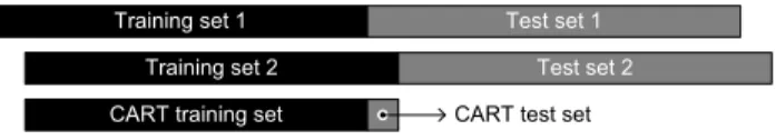
Training set 1 Training set 2
Test set 1 Test set 2
1 2 3 4 5 6 7 8 9 10 11 12 13 14 15 16 17 18 19 20 21 22 23 24 25 CART training set CART test set
Period
Figure 5: Graphical representation of training and test sets.
Customer purchase information from May 2004 up to and including May 2006 was available. Recency, frequency, and monetary (RFM) variables for the DTMC and e-CLV model were calculated for every month. This resulted in 25 periods with RFM variables for every customer.
As was explained earlier, these RFM variables are defined differently for the DTMC model and the CLV model. e-CLV uses aggregated variables, whereas DTMC uses per-period variables. Moreover, the DTMC models only uses records with actual purchases and records in which cus-tomers enter the end state. Cuscus-tomers enter this state after 6 periods of inactivity.
4.2
Model building
Model training consists of two separate steps. First the decision tree has to be trained. Data from periods 2 through 12 is used to train this tree and period 13 is used to test it. The decision tree is then used to define the states for the Markov matrix.
The second step calculates the reward vector and the Markov matrix, enabling the calculation of CLV. To com-pare CLV predictions across time two training and test sets are used for this second step. The states for the Markov matrix are kept identical for both sets in order to enable comparison of CLV’s per state across time. The reward vector is calculated from the training data and state defi-nitions. A graphical representation of the used training and test sets is given in Figure 5. Periods 1 to 12 will be train-ing set 1, periods 2 to 13 traintrain-ing set 2, periods 13 to 24 test set 1, and periods 14 to 25 test set 2. Furthermore, both the ‘lost-for-good’ en the ‘semi-lost’ scenarios, which were introduced earlier, are modeled, resulting in slightly different Markov matrices. All our modeling is done us-ing the free statistical software package R, available from http://cran.r-project.org/.
Before training the decision tree, outliers were deleted from the dataset. We chose to delete all rows that had a monetary value bigger or smaller than three standard devi-ations from the mean in the training period. This resulted in removing 176 records with values larger than 435 on a total of 24482 records.
Next two CART parameters were chosen appropriately, the complexity parameter and the minimum number of records per leaf. The CART tree should have a high accuracy, with the restriction of keeping the tree size down. We chose 250 records as a minimum per leaf, being approximately 1% of the data. Subsequently, the complexity parameter was var-ied and 0.0001, the value giving tree with the highest accu-racy, was chosen.
Now that the decision tree is found the reward vector for training set 1 and 2, as described above and displayed in Figure 5, has to be calculated. Each leaf in the decision tree can be seen as a state. For each state the associated
monetary value is calculated by averaging over all records in this state except outliers. Thus for training set 1 all records from period 1 to 12 are used and for training set 2 all records from period 2 to 13 are used. The next step is to calculate Markov matrices for both data sets.
For both training sets the Markov matrices are calculated. First the state sequence of every customer is determined. The filtered records are also included again, since no outlier filtering is necessary when calculating the Markov matrices. The state sequence then is determined by assigning a state number to every period for every customer using the state definitions as described above. The Markov matrices for both data sets are then determined by counting the number of transitions, as described above.
Using the constructed DTMC models average CLV’s of current and prospective customers can be predicted. By us-ing the number of current customers in every state, customer equity for this group can be calculated. When the number of new customers is estimated customer equity can also be calculated for this group. To calculate these values we use a discount factor of 1% per month.
4.3
Evaluation metric
The results of our experiments will be evaluated by com-paring actual net present values with our predicted CLV’s.
Net present value. Predicted CLV is compared to the realized value by a net present value (NV) calculation over the test period. NV can be seen as the ‘target value’ for CLV – it represents the discountedactualaggregated spending by a customer: NVi= T X t=1 Ait (1 +d)t, (10)
whereNViis the net present value of customeri(i= 1, . . . , I),
Aitis the amount spend by customer iin periodtanddis
the discount factor.
Now that NV of every customer is known NV per state and total NV can be calculated. The relative difference between CLV and NV values will be used to measure the accuracy of the tested models. The difference is thus calculated as
E=|1−CLV/NV|, (11) and should be as small as possible.
4.4
Benchmark models
Our model performance will be tested against two bench-mark models, a naive model and the e-CLV model.
Naive model. Our naive model assumes customer be-havior remains unchanged in every period. Thus, the T -period ahead customer equity is estimated simply by sum-ming the current sales T times and discounting each term appropriately CE= T X t=1 Sales0 (1 +d)t, (12)
whereSales0are the sales in the baseline period.
e-CLV model. As explained earlier, the e-CLV model uses aggregated RFM variables. These variables have to be discretized in order to be applicable. Recency is discretized into 7 categories. Frequency was given an imposed max-imum bound of 6, with 6 indicating 6 or higher. And the monetary amount was discretized into 6 categories, category
State Recency Frequency Monetary 1 Monetary 2 begin - - 0 0 1 ≥1 = 2 85.9 85.8 2 = 0 = 2 104.5 103.2 3 - ≥3 142.6 141.8 4 = 0 = 1 59.2 58.1 5 = 1 = 1 47.5 47.5 6 ≥2 = 1 43.4 43.4 7 = 0 = 6 0 0
Table 6: Recency, frequency and average monetary values per state for training sets 1 and 2, found using the CART decision tree.
1 running from 0 to 100, 2 from 100 to 200, 3 from 200 to 300, 4 from 300 to 400, 5 from 400 to 500, and 6 500 and above.
With these RFM variables the e-CLV model is trained. The discretized variables give rise to 7·6·6 = 252 states, plus a begin state. The state sequence in the training data sets are counted to calculate the Markov matrix. Using the counts, Markov matrices for the ‘lost-for-good’ and ‘semi-lost’ scenarios are calculated as in the DTMC model. ([4] only uses the ‘lost-for-good’ scenario.)
Average monetary values for the reward vector are calcu-lated the same way as with the DTMC model. The added monetary amount is averaged over all customers in every state. Thus only states with a recency of 0 may have a value higher than 0 associated with it, since these are the only states in which actual purchases took place. For states without observations we estimated the reward to be the av-erage reward over all observations with recency 0. Note that Pfeifer and Carraway tackle this problem by using expert knowledge to construct the reward vector [6]. The model in [4] is not clear about the net contributions of the reward vector, but this is probably also the average of the training set due to the large state space.
5.
RESULTS
This section presents the results of the experiments de-scribed in the previous section.
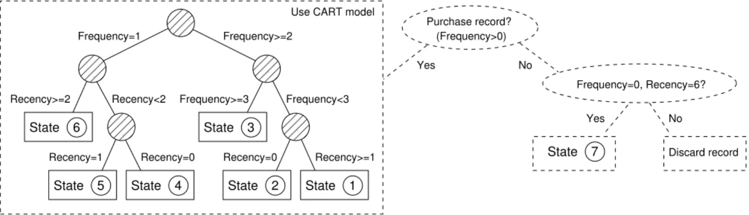
Decision tree step. The resulting decision tree is shown in Figure 6. Six value segments were identified by the tree. These groups are numbered 1 through 6. Group 7 represents the end state. All state definitions as well as the average monetary values for both training sets can be found in Table 6. The monetary values show a logical pattern, states with higher frequencies have higher values. Some variation is captured through recency as well, however. States 1 and 2 differ only in recency for instance. State 7, which functions as the end state, logically has a value of 0 associated with it.
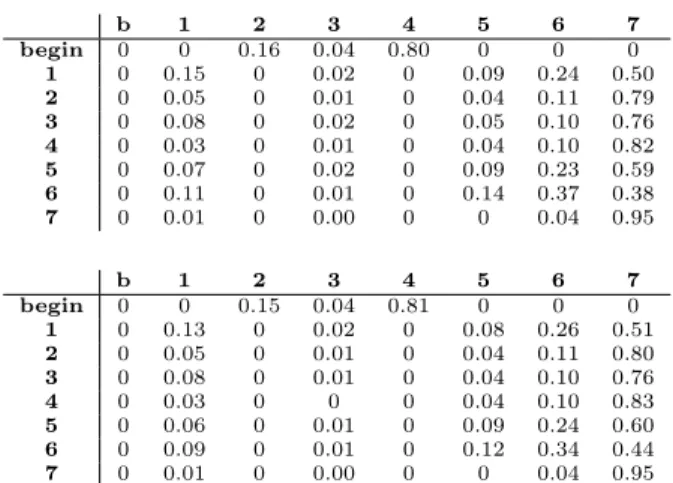
Markov chain step. After generating the sequence data for both training sets and counting the transitions the un-corrected Markov matrices were found. After correction the Markov matrix for the semi-lost scenario for both training set 1 and 2 are shown in Figure 7. For the lost for good scenario the probability of going to state 7 from state 7 is 1 instead of 0.95 for both matrices.
When looking at the Markov matrices the large transi-tion probabilities to state 7 are especially interesting. These values indicate that customers are not very loyal to this company. Furthermore state 6 seems a popular state, be-cause switching probabilities to this state from the others
b 1 2 3 4 5 6 7 begin 0 0 0.16 0.04 0.80 0 0 0 1 0 0.15 0 0.02 0 0.09 0.24 0.50 2 0 0.05 0 0.01 0 0.04 0.11 0.79 3 0 0.08 0 0.02 0 0.05 0.10 0.76 4 0 0.03 0 0.01 0 0.04 0.10 0.82 5 0 0.07 0 0.02 0 0.09 0.23 0.59 6 0 0.11 0 0.01 0 0.14 0.37 0.38 7 0 0.01 0 0.00 0 0 0.04 0.95 b 1 2 3 4 5 6 7 begin 0 0 0.15 0.04 0.81 0 0 0 1 0 0.13 0 0.02 0 0.08 0.26 0.51 2 0 0.05 0 0.01 0 0.04 0.11 0.80 3 0 0.08 0 0.01 0 0.04 0.10 0.76 4 0 0.03 0 0 0 0.04 0.10 0.83 5 0 0.06 0 0.01 0 0.09 0.24 0.60 6 0 0.09 0 0.01 0 0.12 0.34 0.44 7 0 0.01 0 0.00 0 0 0.04 0.95
Figure 7: Transitions probabilities for the semi-lost scenario for training set 1 (top) and 2 (bottom).
state count avg NV avg CLV avg CLV (semi) (lost) begin 0 43 72.2 72.2 1 450 34.4 37.9 37.1 2 1135 10.6 16.1 14.8 3 293 18.7 20.2 19.0 4 7579 9.1 13.7 12.4 5 294 30.9 29.4 28.5 6 1589 30.1 42.9 42.3 7 11226 5.0 3.4 0 total 22566 215132 260369 208799
Table 7: Results for test set 1. For each state, the number of customers, average NV, average CLV for the semi-lost scenario and average CLV for the lost for good scenario are shown. Aggregate results are shown in the last row.
are relatively high. For instance 0.24 from state 1 to state 6. Differences between both matrices are rather small and their effect on CLV’s is therefore hard to predict. Take for example the switching probabilities from the begin state to the others. The probability of going to state 2 decreases from 0.16 to 0.15 and going to state 4 it increases from 0.80 to 0.81. Overall this analysis shows that customer behav-ior is complex, as migration is not limited to segments with similar monetary value.
CLV results. Combining the results of the decision tree step and the Markov chain step resulted in the CLV’s shown in Tables 7 and 8. A quick look learns that the NV values are more or less matched by the CLV’s. See for instance state 1 in Table 7 where average NV is 34.4, average CLV is 37.9 for the semi-lost scenario and average CLV is 37.1 for the lost for good scenario.
Another interesting thing to note is the number of cus-tomers per state. State 7 is the biggest group for both test sets with respectively 11226 and 12912 customers. The large increase in this number indicates that a lot of customers are becoming inactive. Especially because the other states do not have an increasing number of customers except state 6, this indicates a retention problem for the company. Total CLV’s are shown in the bottom row of Tables 7 and 8. The quality of these estimates will be further discussed below, where our model is compared to the benchmark results.
Net present value comparison. The DTMC models is compared to the Naive and e-CLV models using the
evalua-Purchase record? (Frequency>0)
Frequency=0, Recency=6?
7 5
State State 4 State 2 State 1
6 State State 3 Yes No Yes No Discard record State
Use CART model Frequency=1 Recency<2 Recency=0 Recency=0 Frequency<3 Frequency>=2 Recency>=2 Frequency>=3 Recency>=1 Recency=1
000
000
000
111
111
111
000
000
000
111
111
111
00
00
11
11
000
000
000
111
111
111
000
000
000
111
111
111
Figure 6: Decision tree resulting from the training data of period 2 to 12. The encircled numbers indicate the states for the Markov step.
state count avg NV avg CLV avg CLV (semi) (lost) begin 0 43.7 69.6 69.6 1 394 31.5 34.9 34.1 2 906 10.6 15.2 14.0 3 217 18.3 19.2 18.1 4 7127 9.2 12.6 11.3 5 286 29.2 27.4 26.5 6 1725 30.7 36.7 36.0 7 12912 5.0 3.4 0 total 23567 217158 236204 180584
Table 8: Results for test set 2.
set 1 E set 2 E avgE
NV 215132 0.0% 217158 0.0% 0.0% DTMC (semi) 260369 21.0% 236204 8.8% 14.9% DTMC (lost) 208799 2.9% 180584 16.8% 9.9% Naive 384935 78.9% 207893 4.3% 41.6% e-CLV (semi) 231091 7.4% 211213 2.7% 5.1% e-CLV (lost) 127398 40.8% 105303 51.5% 46.1%
Table 9: NV, CLV and relative errors (see Eqn. (11)) for all tested models for both test sets.
tion metric described in the previous section. Table 9 shows the results on individual test sets and the average error over these sets. On the first test set the DTMC model with the lost for good scenario performs best with an error of 2.9%, the semi-lost scenario e-CLV model is best on the second test set with 2.7% error. On average this model also per-forms best, with an error of 5.1%, followed by the DTMC lost for good model with 9.9% error and the DTMC semi-lost model with 14.9%. The Naive model and e-CLV semi-lost for good model perform substantially worse with respective average errors of 41.6% and 46.1%.
Discussion of the results. From our analysis a mixed conclusion can be drawn. First the Naive model seems to make a more or less random guess. For the first test set CLV is highly overestimated by this method and the estimate for the second test set is close by. Another shortcoming is the lack of discrimination between customers, because the other models have such a possibility. Overall the Naive model gives a quick, but dirty, estimate of total CLV.
The other models do a better job. The semi-lost scenario e-CLV model performs best overall in terms of accuracy. The e-CLV lost for good model performs way worse, with a very high average error. The difference between both DTMC
model scenarios is much smaller. The DTMC lost for good model has the lowest average error and the DTMC semi-lost scenario shows the best trend prediction. Both models perform reasonably well compared to the semi-lost e-CLV model.
The main advantage of the DTMC models as opposed to the e-CLV models is the much smaller number of groups. Interpreting the customer groups is easier for the DTMC model which aids practical actionability. Take for instance the conditions of the variables given in Table 6 and the av-erage CLV’s of Tables 7 and 8. Given these values it can be concluded that customers who less recently bought some-thing are more valuable, because the recency of states 1, 5, and 6 are at least 1 and their CLV’s are all higher than states 2,3, and 4 which can have recency 0. Put differently, customers who bought something in at least two period are worth more, because customers can not return to states 2 or 4, due to the 0 recency. It is much more difficult to draw such a conclusion for the e-CLV model.
6.
SUMMARY, CONCLUSIONS AND
DISCUSSION
This paper discussed a customer lifetime value (CLV) model that can be used in e-commerce environments to monitor web site success, provide marketing diagnostics and generate insight. Moreover, a CLV model makes general marketing efforts more accountable – efforts that increase the customer equity (total CLV) are justifiable, others are not.
Because Internet retailing generates a lot of customer data through the extensive use of technology, it should be possible to measure CLV by historical data. In the literature recency, frequency and monetary (RFM) variables are combined with Markov models to calculate CLV [6]. The inclusion of more RFM variables specific to e-commerce into these Markov CLV models was studied by [4], which proved to perform well.
A shortcoming of these studies is the exponential increase of states with the number of variables. The interpretation of the states becomes quite cumbersome this way. A segmen-tation of the customer records of every period could prevent this. For this reason we developed the DTMC model, based on decision trees and Markov chains.
Using only a few variables concerning customer behavior reasonable CLV estimates can be made. This is true for both
the e-CLV model and the DTMC model. These estimates can be used to monitor the overall business effectiveness over time.
One of the shortcomings of the DTMC model is the, rather inelegant, deletion of records. Records without a reward are deleted from the data. This gives some complications with regards to the formulation of the CLV equation. Using different input variables may prevent this problem.
A general point of discussion about our research is the number of variables used. Only RFM variables are used to test a model on applicability in an e-commerce domain. Use of more variables specific to e-commerce and data mining could improve the model. Different CLV drivers may exist in different industries, and this can easily be incorporated in our model.
Using decision trees for grouping the RFM variables was a deliberate choice. Their interpretability greatly aids in explaining the results to decision makers. Especially when incorporating more data this may be very useful for the man-ager’s understanding. When for instance demographic data are also included, it could be the case that there are cer-tain segments of only males, who are very profitable, which would be very useful information for managers. Moreover, the decision tree approach leads to a low number of seg-ments, which can be individually targeted by marketing ac-tions. We encountered business users who appreciate this actionability.
Another future research direction is the formulation of other segment level CLV models. An example could be to replace the decision tree by using a different clustering pro-cedure. (Although general clustering procedures lack the interpretability of CART.) Furthermore the clustering step and Markov chain step could be done simultaneously to get an optimal partitioning according to CLV’s. Finally, it could be worthwhile to adapt the CART algorithm such that it finds customer segments that give the highest possible ac-curacy when combined with a Markov model for predicting CLV. We are currently exploring this option.
7.
ACKNOWLEDGMENTS
We thank ISM e-Company (http://www.ism.nl) for pro-viding us with access to the data of one their clients. (The client wishes to remain anonymous.) We thank the We thank the ‘Vereniging Trustfonds Erasumus Universiteit Rot-terdam’ for a travel grant.
8.
REFERENCES
[1] P. D. Berger and N. I. Nasr. Customer lifetime value: Marketing models and applications.Journal of Interactive Marketing, 12(1):17–30, 1998.
[2] L. Breiman, J. Friedman, R. Olshen, and C. Stone.
Classification and Regression Trees, 2nd Edition. Chapman & Hall, NY, 1996.
[3] F. R. Dwyer. Customer lifetime valuation to support marketing decision making.Journal of Direct Marketing, 11:6–13, 1997.
[4] O. Etzion, A. Fisher, and S. Wasserkrug. e-CLV: A modeling approach for customer lifetime evaluation in e-commerce domains, with an application and case study for online auction.Information Systems Frontiers, 7:421–434, 2005.
[5] J. W. Palmer. Web site usability, design, and performance metrics.Information Systems Research, 13(2):151–167, 2002.
[6] P. E. Pfeifer and R. L. Carraway. Modeling customer relationships as Markov chains.Journal of interactive marketing, 14:43–55, 2000.
[7] S. Rosset, E. Neumann, U. Eick, and N. Vatnik. Customer lifetime value models for decision support.
Data mining and knowledge discovery, 7:321–339, 2003.
[8] R. T. Rust, K. N. Lemon, and V. Zeithaml. Return on marketing: using customer equity to focus marketing strategy.Journal of marketing, 68:109–127, 2004. [9] R. T. Rust, V. Zeithaml, and K. N. Lemon.Driving
customer equity - How customer lifetime value is reshaping corporate strategy. The free press, 1230 Avenue of the americas, New York, NY 10020, 2000. [10] E. Schonberg, T. Cofino, R. Hoch, M. Podlaseck, and
S. L. Spraragen. Measuring success.Communications od the ACM, 43(8):53–57, 2000.
[11] R. K. Srivastava, S. T. A., and L. Fahey. Marketing, business processes, and shareholder value: an organizationally embedded view of marketing activities and the discipline of marketing.Journal of marketing, 63:168–179, 1999.
[12] Forrester Research Inc. The state of retailing online 2006 – a shop.org survey, 200.
http://www.shop.org/press/06/052306.asp. http://www.forrester.com/SORO. Accessed on 6/21/2006.
[13] U.S. Census Bureau. Quarterly retail e-commerce sales 3rd quarter 2006. Web-site, 2006.http: //www.census.gov/mrts/www/data/html/06Q3.html. Accessed on 12/15/2006.
[14] R. Venkatesan and V. Kumar. A customer lifetime value framework for customer selection and resource allocation strategy.Journal of marketing, 68:106–125, 2004.