Classication and Clustering Using Intelligent Techniques: Application to Microarray Cancer Data

(1)

Classification and Clustering

Using Intelligent Techniques:

Application to Microarray Cancer Data

Anita Bai

Department of Computer Science and Engineering

National Institute of Technology Rourkela

(2)

Using Intelligent Techniques:

Application to Microarray Cancer Data

Thesis submitted in partial fulfillment of the requirements for the degree of

Master of Technology

in

Computer Science and Engineering

(Specialization: Software Engineering)

by

Anita Bai

(Roll No: 211CS3291)

under the supervision of

Prof. S. K. Rath

Rourkela, Odisha, 769 008, India

(3)

Rourkela-769 008, Odisha, India.

Certificate

This is to certify that the work in the thesis entitled“Classification and Clus-tering Using Intelligent Techniques: Application to Microarray Can-cer Data” byAnita Baiis a record of an original research work carried out by her under my supervision and guidance in partial fulfillment of the requirements for the award of the degree of Master of Technology with the specialization of Software Engineering in the department of Computer Science and Engineering, National Institute of Technology Rourkela. Neither this thesis nor any part of it has been submitted for any degree or academic award elsewhere.

Place: NIT Rourkela (Prof. S. K. Rath)

Date: 3 June 2013 Professor, CSE Department

(4)

I am grateful to numerous local and global peers who have contributed towards shaping this thesis. At the outset, I would like to express my sincere thanks to Prof. Santanu Kumar Rath for his advice during my thesis work. As my super-visor, he has constantly encouraged me to remain focused on achieving my goal. His observations and comments helped me to establish the overall direction of the research and to move forward with investigation in depth. He has helped me greatly and been a source of knowledge.

I am very much indebted to Prof. Ashok Kumar Turuk, Head-CSE, for his continuous encouragement and support. He is always ready to help with a smile. I am also thankful to all the professors of the department for their support.

I am really thankful to my all friends, especially my ‘puzzle’ group of best friends. I would also like to thank all the Ph.D. scholars and especially to Ph.D. scholars Swati Vipsita and Yeresime Suresh for helping me and giving advise. My sincere thanks to everyone who has provided me with kind words, a welcome ear, new ideas, useful criticism, or their invaluable time, I am truly indebted.

I must acknowledge the academic resources that I have got from NIT Rourkela. I would like to thank administrative and technical staff members of the Depart-ment who have been kind enough to advise and help in their respective roles.

Last, but not the least, I would like to dedicate this thesis to my family, for their love, patience, and understanding.

Anita Bai Email : [email protected]

(5)

Abstract

Analysis and interpretation of DNA Microarray data is a fundamental task in bioinformatics. Feature Extraction plays a critical role in better performance of the classifier.

We address the dimension reduction of DNA features in which relevant features are extracted among thousands of irrelevant ones through dimensionality reduc-tion. This enhances the speed and accuracy of the classifiers. Principal Component Analysis (PCA) is a technique used for feature extraction which helps to retrieve intrinsic information from high dimensional data in eigen spaces to solve the curse of dimensionality problem. The curse of dimensionality means n >> m, where n is a large number of features and m is a small number of samples (may be too less). Neural Networks (NN) and Support Vector Machine (SVM) are implemented and their performances are measured in terms of predictive accuracy, specificity, and sensitivity. First, we implement PCA for significant feature extraction and then FFNN trained using Backpropagation (BP) and SVM are implemented on the reduced feature set.

Next, we propose a Multiobjective Genetic Algorithm-based fuzzy clustering technique using real coded encoding of cluster centers for clustering and clas-sification. This technique is implemented on microarray cancer data to select training data using multiobjective genetic algorithm with non-dominated sorting (MOGA-NSGA-II). The two objective functions for this multiobjective techniques are optimization of cluster compactness as well as separation simultaneously. This approach identifies the solution i.e. the individual chromosome which gives the optimal value of the compactness and separation. Then we find high confidence points for these non-dominated set using a fuzzy voting technique. Support Vec-tor Machine (SVM) classifier is further trained by the selected training points which have high confidence value. Then remaining points are classified by trained SVM classifier. Finally, the four clustering label vectors through majority vot-ing ensemble are combined, i.e., each point is assigned a class label that obtains

(6)

been compared to MOGA-BP, SVM, BP. The performance are measured in terms of Silhoutte Index, ARI Index respectively. The experiment were carried on three public domain cancer data sets, viz., Ovarian, Colon and Leukemia cancer data to establish its superiority.

Keywords: Cancer Classification; Feature Reduction; Multiobjective genetic al-gorithm; Neural Network; Pareto-optimality; Principal components; Support Vec-tor Machine(SVM)

(7)

List of Tables

3.1 Accuracy vs. No. of PC’s using PCA-SVM (Leukemia Cancer data set) . . . 35 3.2 Classification Results: SVM Kernels . . . 36 3.3 Classification Results: Traditional BP, SVM, BP, and

PCA-SVM . . . 36 4.1 PARAMETER VALUES FOR MOGA-SVM . . . 53 4.2 Performance of Fuzzy Compactness (π) and Fuzzy Seperation (sep) 55 4.3 Classification Results: SVM Kernels with MOGA . . . 56 4.4 Classification Results: Traditional BP, SVM, BP, and

MOGA-SVM . . . 56 4.5 Comparison of different algorithms in terms of silhouette score and

(12)

(13)

Chapter 1

Introduction

1.1

Introduction

Much research is being done in the academics as well as the industries towards the application of bioinformatics that uses computational approaches to solve bio-logical problems. The goal of this field is to retrieve, analyze and interpret the vast and complex genomic data sets that are uncovered in large volumes of genes in molecular biology. Biological data mining posses various challenges like gene dis-covery, drug disdis-covery, gene finding, revealing unknown relationship with respect to structure and function of genes to understand biological systems. This field faces demands for immediate prediction and classification due to the availability of DNA cancer data, structure information of proteins and microarray technology to provide dynamic information about thousand of genes in data. The aims of Bioinformatics are:

1. To organize data in a way that allows researcher and practitioners to access existing information and to submit new entries as they are produced. 2. To develop tools, softwares and resources that aid in the analysis and

man-agement of data.

3. To use this data to analyze and interpret the results in a biologically mean-ingful manner.

4. To help practitioners in the pharmaceutical industry in understanding the microarray cancer data structures which helps the disease prediction easy.

(14)

1.1.1

DNA

DNA (also known as deoxyribonucleic acid) is the hereditary material in humans and almost all other organisms. DNA is the material present in our cells that makes up our genes. Genes carry and follow the instructions our bodies use to grow and function. Nearly every cell in a persons body has the same DNA. Most DNA is presented in the cell nucleus (where it is called nuclear DNA), and a less amount of DNA can also be found in the mitochondria (where it is called mitochondrial DNA or mtDNA). The information under DNA is stored as a code made up of four chemical bases: adenine (A), guanine (G), cytosine (C), and thymine (T). Sequence of nucleotides in a DNA is defined by the sequence of a gene, which is encoded in the genetic code i.e. 4 standard of nucleotides. One strand is a polynucleotide (a sequence of nucleotides of 4 types); the second strand has their complementary base pairs (A = T , C = G). DNA consists of 2 strands of nucleotides forming a double helix structure. DNA nucleotides vary depending on 4 possible nitrogenous bases A,C,T,G. In the basis of accurance of pattern ,find the gene values and partition in classes.

1.1.2

Cancer Classification

Cancer classification is a challenging task of bioinformatics. For cancer classifi-cation we concentrate on behaviour of DNA microarray. The Microarray technol-ogy (DNA microarray) [1] allows us to measure the expression levels of thousands of genes simultaneously, providing great chance for cancer diagnosis and progno-sis. A microarray cancer data having ‘p’ genes and ‘n’ samples (observations) are typically organized in a 2D matrix X = [aij] of sizep×n. Each element aij gives

the expression level of the ith _{gene at the}_jth _sample.

Xn×p =         f1 f2 · · · fp s1 a11 a12 · · · a1p s2 a21 a22 · · · a2p .. . ... ... . .. ... sn an1 an2 · · · anp         samples×f eatures

(15)

1.1 Introduction

xnp = sample s1 have expression measures for genes from f1 to fp .

si = (ai1, ai2, ..., aip)− gene expression profile/feature vector for sample i

fj = set of samples aij for feature j.

where, i = 1, . . . , n. and j= 1,..., p.

When microarray datasets are organized as samples versus gene fashion, then they are very helpful for classification of different types of tissues and identifica-tion of those genes whose expression levels are good diagnostic indicators. The microarray datasets, where the tissue samples represent the samples from cancer-ous (malignant) and non-cancercancer-ous (benign) cells, the classification of them will result in binary cancer classification. On the other hand, if the samples are from different subtypes of cancer, then it becomes the problem of multi-class cancer classification.

The task for cancer classification are of two aspects: identifying new cancer classes and assigning genes to known classes, which are called class discovery and class prediction [2]. DNA microarray technology is a promising tool for cancer diagnosis. It generates large-scale gene expression profiles that include valuable information on organization as well as cancer [3].

Classification, or supervised learning is one of the major data mining processes. Classification is concerned with assigning memberships to samples based on su-pervised expression patterns. The classification of data has two stages. In the first stage, a model is determined from a set of data called training data (the classes of which have been established beforehand). This model is shown as rules or math-ematical formulae. In the second stage the correctness of the evolved model is estimated. This is done by studying the results of the evolved models function on a set of data (test data). The classes of the test data also are determined beforehand. DNA microarray cancer data classification, which determines a new cancer data belongs to which class it helps to find types of cancer. The aim of classification is to predict target class for the given unknown input. There are many approaches available for classification tasks such as statistical techniques, decision trees, fuzzy logic, neural networks etc.

(16)

1.1.3

Cancer Clustering

Clustering an unsupervised classification technique, is the process of grouping or organizing a set of objects into distinct group based on some similarity or dissimilarity measure among the individual objects, such that the objects in the same group are more similar to each other than those in other groups. Clustering, an important microarray analysis tool, is used to identify the sets of genes with similar expression profiles. Clustering methods partition a set of objects into groups based on some similarity/dissimilarity metric where the value of may or may not be known a priori. Clustering can be mainly divided into two types Hard Clustering and Soft Clustering.

Hard Clustering

Hard Clustering is based on classical set theory, and in this method of cluster-ing the object either does or does not belong to a cluster [4]. If each data point is assigned to a single cluster, then the clustering is called crisp (hard) clustering. In Hard clustering data is partitioned into specified number of mutually exclu-sive subsets. Using hard partitioning for algorithms based on analytic functional causes difficulties because hard partitioning is discrete in nature and also since this functional are not differentiable.

Soft (Fuzzy) Clustering

If a data point has certain degrees of belongingness to each cluster, the par-titioning is called fuzzy. In Soft Clustering [4], unlike hard clustering the object doesn’t belong to a particular cluster rather an object belongs to more than one cluster simultaneously with different degree of membership and with every object there is an associated set of membership levels. The membership level indicates the strength of the association between that object and a particular cluster. Ob-jects on the boundaries between several classes are assigned a membership value between 0 and 1 indicating partial membership rather than they are not forced them to fully belong to a single cluster.

(17)

1.2 Basic Concepts of Artificial Neural Network

1.2

Basic Concepts of Artificial Neural Network

Neural networks, with their remarkable ability to derive meaning from com-plicated or imprecise data, can be used to extract patterns and detect trends that are too complex to be noticed by either humans or other computer techniques. Advantages of ANN include:

1. Adaptive learning: An ability to learn how to do tasks based on the data given for training or initial experience.

2. Self-Organization: An ANN can create its own organization or representa-tion of the informarepresenta-tion it receives during learning time.

3. Real Time Operation: ANN computations may be carried out in parallel, and special hardware devices are being designed and manufactured which take advantage of this capability.

4. Fault Tolerance via Redundant Information Coding: Partial destruction of a network leads to the corresponding degradation of performance. However, some network capabilities may be retained even with major network damage.

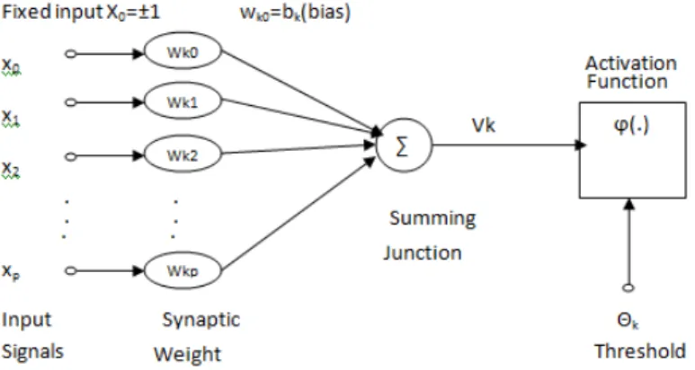
Figure 1.1: The Mathematical Model of Artificial Neuron

An ANN is typically defined by three types of parameters:

1. The interconnection pattern i.e. the synaptic weight between different layers of neurons.

(18)

2. The learning process for updating the weights of the interconnections. 3. The activation function that converts a neuron’s weighted input to its output

activation.

In mathematical form for a given artificial neuron, let there be m + 1 inputs with signals x0 to xm with associated synaptic weights w0 through xm. Usually, the

x0 input is assigned the value +1, which makes it a bias input with wk0 =bk=0.

Hence only m actual inputs to the neuron, from x1 to xm. The output of kth

neuron is defined by Y which is computed using an activation functionϕ(x) :

yk =ϕ( m X j=0 wjxj) (1.1) Where vk = Pm

j=0wjxj is the summing function in which each input is multiplied

by the associated synaptic weight and then added. The mathematical model is illustrated in Fig 1.3.

1.2.1

Activation Function

In computational networks, the activation function defined as the function which generates the output for a given set of inputs. It acts as a non-linear filter, which is one of the important parameters of ANN that characterizes the architecture. The behavior of neural networks depend upon the choice of activation function [5], i.e., how they map input data to output data considering weights of those intercon-nections. Activation functions with a bounded range are often called squashing functions.

Activation function can be of following types:

1. Linear function: Here the input units use the identity function. A linear combination formed where the weighted sum input of the neuron with a linearly dependant bias becomes the system output. Specifically:

g(y) =y where y =Xwixi+b

2. Threshold function: This function is also known as Step function or Heav-iside function. Here sum is compared with a threshold value θ.

(19)

1.2 Basic Concepts of Artificial Neural Network    g(x) = 1 if(x≥θ) g(x) = 0 if(x < θ)

This kind of function is often used in single layer networks and called as binary step function.

3. Signum function: This function is also known as Quantizer function. It is especially advantageous for use in neural networks because it is easy to dif-ferentiate and can dramatically reduce the computation burden for training. It applies to applications whose desired output values are between -1 and 1.

 



g(x) = 1 if(x≥θ)

g(x) = −1 if(x < θ)

4. Sigmoidal function: This function is a continuous function that varies between asymptotic values 0 and 1 or 1 and -1. The sigmoidal function can be described as

g(x) = 1 1 +e(−αx)

whereα is the slope parameter, which adjust the abruptness of the function due to the change in asymptotic values.

5. Ramp function: The ramp function combines the step function with a linear output function. As long as the activation is smaller than the threshold value θ1, the neuron shows the output yi = 0; if the activation exceeds the

threshold valueθ2, the output isyi=1. The neuron’s output for activations in

the interval between the two threshold valuesθ1≤zi( x ,wi≤θ2) is determined

by a linear interpolation of the activation.

yi = f(zi) =          0 if(zi ≤θ1) (zi−θ1)·_θ₂₋1_θ₁ if(θ1 ≤zi ≤θ2) 1 if(zi ≥θ2)

Activation functions for the hidden layers are needed to deploy non-linearity into the networks which makes multi-layer networks so powerful. The sigmoid function

(20)

always been the common choice, either in symmetric [-1, 1] or asymmetric [0, 1] form. The sigmoid function is global in nature i.e. it divides the feature space into two halves, one for the response is approaching 1 and another for (0/-1). Hence it is very efficient for making indiscriminate target value distribution in the feature space.

1.2.2

NN Architecture

• Single layer Feed Forward Network: This type of network comprise of two layers, namely the input layer and output layer. Feed-forward ANNs (figure ) allow signals to travel one way only; from input to output. There is no feedback (loops) i.e. the output of any layer does not affect the previous layer neurons. Feed-forward ANNs tend to be straight forward networks that associate inputs with outputs. They are extensively used in pattern recognition. The input layer neuron receives the input signals and the output layer neuron receives the output signals. The interconnected links carry the synaptic weights. Despite the two layers, the network is termed single layer since it is the output layer alone which performs computation. The input layer merely transmits signals to the output layer hence, the name single layer feed forward network. Such a network is said to be feed forward or acyclic in nature.

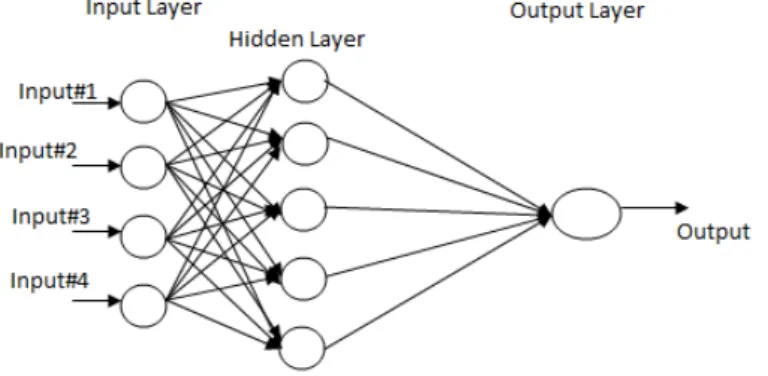
• Multilayer Feed Forward Network: This class of feed forward neural network distinguishes itself by the presence multiple layers. The architecture of this network posses input layer, output layer and one or more intermediary layers called hidden layers, whose computation nodes are correspondingly called hidden neurons or hidden units. The function of hidden neuron is to intervene between the external input and network output in some useful manner. By adding one or more hidden layers, the network is enabled to extract higher order statistics i.e. valuable when size of input layer is large. A multilayer feed forward network with m input neurons, h1 neurons in the first hidden layer, h2 neurons in the second hidden layer and n output

(21)

1.2 Basic Concepts of Artificial Neural Network

neurons in the output layer is referred as m-h1-h2-n network. The neural network is said to be fully connected if every node in each layer is connected to every other node in adjacent forward layer. If some of the communication links are missed then the network is a partially connected network. Fig illustrates a multilayer feed forward network:

Figure 1.2: Multilayer Feedforward Network

• Recurring Network: These networks differ from feed forward network architectures in the sense that there is at least one feedback loop. Thus, in these networks there could exist one layer with feedback connections .There could also be neurons with self-feedback links i.e. the output of a neuron is feedback into itself as input. The presence of feedback loops in the recurrent structure has a profound impact on the learning capability of the network and its performance.

(22)

1.2.3

Learning Paradigm

Learning is a process by which the free parameters of neural network are adapted through a process of stimulation by the environment in which the network is embedded. It can be broadly classified into 3 categories: supervised learning, unsupervised learning, reinforcement learning.

• Supervised Learning: It is also referred as learning with a teacher. For every input pattern a desired output pattern (targeted output) is provided. The difference between the computed output and desired output generates the error in the network, which used to change network parameters for the improvement in networks performance. Error-correction learning and stochastic learning are generally used in supervised learning process. Its task often include function approximation problem (regression) i.e. a given training data consisting of pairs of input patterns x, and corresponding tar-get t, the goal is to find a function f(x):x → y that matches the desired response (y) for each training input.

• Unsupervised Learning: In this paradigm no teacher is to oversee the learning process i.e. no target output is given for the network. Hence the network learns by its own through discovering and adapting the features, reg-ulations, correlations or categories in the input pattern automatically. It usu-ally performs the same task as an auto-associative network does, compressing the information from inputs. It is also referred to as self-organization, that it self-organizes data presented to the network and detects their emergent collective properties. Paradigms of unsupervised learning are Hebbian learn-ing and Competitive learnlearn-ing. The identification of new tumor classes uslearn-ing gene expression profiles

• Reinforcement Learning: In this learning paradigm, a teacher does not present the expected answer but only indicates if the computed output is correct or incorrect. The learning of an input-output mapping is performed through continued interaction with the environment that will minimize a

(23)

1.4 Motivation

scalar index of performance. The information provided helps the network in its learning process. A reward is given for a correct answer computed and a penalty for a wrong answer.

1.3

Neural Network for Cancer Classification

NN are an effective tool in the field of cancer Classification. In the training stage (Approximation), neural networks extract the features of the input data. In the recognizing stage (Generalization), the network distinguishes the pattern of the input data by the features, and the result of recognition is greatly influenced by the hidden layer. Every instance in any dataset used by machine learning algorithms is represented using the same set of features. The features may be continuous, real coded, categorical or binary.

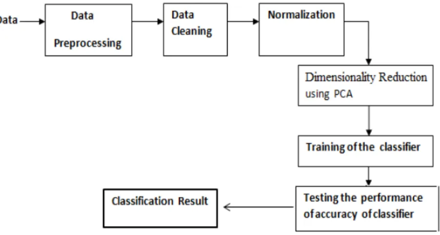
Figure 1.4: Brief overview of the entire process

If instances are given with known labels (the corresponding correct outputs) then the learning is called supervised, in contrast to unsupervised learning, where instances are unlabeled. Learning is usually accomplished by adjustment and modification of the connected synaptic weights.

1.4

Motivation

It is required to develop an intelligent system to classify the microarray cancer data with high accuracy. Many machine learning techniques have been

(24)

success-fully implemented for classification and clustering. In the first stage, training of the classifier is done with known labeled samples. After the classifier is success-fully built, unknown test samples are used to measure the effectiveness of the classifier. Among the soft computing paradigms, Neural Network (NN) approach efficiently handles linear and non-linear data classification tasks. Dimension re-duction used for remove Noisy or irrelevant features which gives negative effect on accuracy of any classifier. Neural networks have been chosen as technical tools for the microarray classification task because extracted features of the DNA data are distributed in a high dimensional space with complex characteristics. SVM are used for cancer classification because correctly separate entities into appropriate classes. The main motivation for dimension reduction are reduce curse of dimen-sionality problem. Different clustering algorithms usually attempt to cluster the gene expression data but in this report multiobjective optimization of cluster va-lidity measures such as compactness and separation among clusters in microarray cancer data has been proposed and computation of cluster modes is costlier than that of cluster means, the algorithm needs to find the membership matrices that takes a reasonable amount of time. However, as fuzzy clustering is better equipped with to handle overlapping clusters.

Two most desirable features of an multiobjective Genetic algorithm:

• Convergence to Pareto optimal front

• Maintenance of Diversity.

1.5

Objective:

In the experiment on genes we can find the gene which are affected by cancer are identified by classification and clustering. Correct prediction of unknown genes or newly discovered mainly concerns the biologists or researchers for prediction of cancers in cell, molecular function, drug discovery, medical diagnosis etc.

• An efficient classification technique needs to be implemented or develop an efficient classifier to correctly classify the unknown genes so that the cancer

(25)

1.6 Thesis Organization

patient are diagonised correctly and this treatment can be done as per the diagnosis.

• To develop an efficient classifier which can classify and cluster the new mi-croarray genes correctly using intelligent techniques and optimizes the result.

• To cluster the unknown genes and optimize cluster compactness and sepa-ration simultaneously for each chromosome.

1.6

Thesis Organization

The rest of the thesis is organized as follows: In Chapter 2, all the efforts in the literature have been focused which describe the various approaches for mi-croarray cancer classification using Backpropagation neural networks, SVM and role of MOGA and NSGA-II in clustering. In Chapter 3, feature extraction and dimension reduction technique and architecture of BPNN and SVM classifier are discussed with their experimental results. In Chapter 4 basic concept of GA, MOGA and NSGA-II is discussed. Implementation of MOGA-SVM for classi-fication and clustering with microarray cancer data and performance measures using Silhout index S(C) and Adjusted Rand Index (ARI) has also been discussed with their simulation results. Finally Chapter 5 concludes the report and gives a platform for further research.

(26)

(27)

Chapter 2

Related Work

In previous work, due to the presence of large number of genes and high com-plexity of biological networks, there is a great need to develop analytical method-ology to analyze and to exploit the information captured by gene expression data. In the pattern layer of Backpropagation Neural Network(BPNN) model, due to the presence of redundant nodes the computational complexity of the network in-creases and so does the computational cost. The performance of Back-propagation training algorithm applied to a feedforward multilayer neural network and its per-formance depend on the activation function and error-correction rule [6]. Feature extraction of microarray genes has a greater impact on its classification and clus-tering as it is taken as input to any network. The use of gene expression data in discriminating two types of very similar cancers acute myeloid leukemia (AML) and acute lymphoblastic leukemia (ALL) presented in [7]. Classification results are reported in [2] using methods other than neural networks. Here, we explore the role of the feature vector in classification. To achieve the best performance with a learning algorithm on a particular training set, a feature subset selection method should be applied. PCA is an orthogonal transformation of the coordinate system in which the data are represented. The new transformed coordinate values by which data are represented are called principal components [8].

Principal component analysis has been applied to analyze gene expression data and to improve cluster quality are studied in [9]. The diagnosis of multiple com-mon adult malignancies could be achieved purely by molecular classification, this is done by using Support vector machine algorithm [10]. Support Vector

(28)

Ma-automatically discovered the distinction between acutemyeloid leukemia (AML) and acute lymphoblastic leukemia (ALL) without previous knowledge of these classes. An automatically derived class predictor was able to determine the class of new leukemia cases are presented in [2]. One particular machine learning al-gorithm, Support Vector Machines (SVMs), has shown promise in a variety of biological classification tasks, including gene expression microarrays are presented in [10], [12]. SVM method and one of its improved version CSVM as the classi-fier gave a better result using gene expression data [13]. The selection of a small subset of genes out of the thousands of genes in microarray data is important for accurate classification of phenotypes are presented in [14]. Multiobjective genetic algorithms gives fast nondominated sorting approach NSGA-II. In this paper we investigate the Goldberg’s notion of non dominated sorting in GA’s along with niche and speciation method to find multiple pareto optimal points simultane-ously [15].

K. Deb et al. presented much better spread of solutions and better conver-gence near the true Pareto-optimal front compared to Pareto-archived evolution strategy and strength-Pareto EA two other elitist MOEAs [28]. Ramaswamy et al. presented tumor gene expression for Multiclass cancer diagnosis [10].

From the related works it has been concluded that Feature extraction for the microarray cancer data is important for classification and clustering. To reduce features from data is important to increase the efficiency of the network, hence a principal component analysis is used for feature reduction. In various paper it has shown that SVM has A greater efficiency in performance of classification as it has various parameter to regularize. Multiobjective genetic algorithms is used to obtain non- dominated solutions .

(29)

(30)

Feature Extraction and Cancer

Classification

3.1

Dimension Reduction

Data analysis causes problem where the data objects have a large number of features which is more prevalent in areas such as multimedia data analysis and bioinformatics. It is often beneficial to reduce the dimension of the data in order to improve the efficiency and accuracy of data analysis [16]. One of the problems with high-dimensional datasets is that, in many cases, not all the measured variables are important for understanding the underlying phenomena of interest. While certain computationally expensive novel methods can construct predictive models with high accuracy from high-dimensional data, it is still of interest in many applications to reduce the dimension of the original data prior to any modelling of the data. To deal with this issue, dimension reduction techniques are often applied as a data pre-processing step or as part of the data analysis to simplify the data model. By working with this reduced representation, tasks such as classification or clustering can often yield more accurate and readily interpretable results, while computational costs may also be significantly reduced.

The motivation for dimension reduction can be summarized as follows:

• The identification of a reduced set of features that are predictive of outcomes can be very useful from a knowledge discovery perspective.

(31)

3.1 Dimension Reduction

increases directly with large number of features.

• Noisy or irrelevant features can have the same influence on classification and clustering as predictive features so they will impact negatively on accuracy.

• Things look more similar on average the more features used to describe them. It shows that the resolution of a similarity measure can be worse in 20D than in a 5D space.

In mathematical terms, the problem can be stated as: we have n observations ,each being a realization of p-dimensional random variable X = (x1, x2, . , xp)

where to find a lower dimensional representation of it, s = (s1,s2, , sk) with k ≤

p, that captures the content in the original data according to some criterion. Here

Xnp is transformed to Xnk . Typically this is a linear transformation Wkp that

will transform each objectxitox01 in k dimensions with meanµ= (µ1, . ,µp) and

covariance matrix P

= (X-µ) (X-µ)T =P

pxp such matrix can be represented by X= {xij:1≤i≤n, 1≤j≤p}.

X_i0 =W Xi (3.1)

3.1.1

Objectives of Feature Extraction

The objectives of feature extraction are many, the major ones are:

• To avoid over fitting and improve model performance.

• To provide faster and more cost-effective models, and

• To gain a deeper insight into the underlying processes that generated the data.

As the data sets have various attributes and due to the huge amount of data we cannot consider all the dataset. So we apply different analysis algorithm to reduce our data sets. So that only few data sets can contribute to the final result. Here we have used a dimension reduction methods i.e Principal Component Analysis (PCA) to reduce the size of data.

(32)

3.1.2

Dimension Reduction using Principal Component

Anal-ysis:

PCA was invented in 1901 by Karl Pearson. Principal component analysis (PCA) is a mathematical procedure that uses an orthogonal transformation to convert a set of observations of possibly correlated variables into a set of values of uncorrelated variables called principal components [17]. Hence the central idea is to reduce the dimensionality of the data set while retaining as much as possible the variation in data set. Principal components (PC’s) are linear transformation of the original set of variables. PC’s are uncorrelated and ordered in such a way that the first few PC’s contain most of the variables in the original data set. The number of PCs are less than or equal to the number of original variables. PCA provides an efficient way to find these components which contribute to the data variation and thus reduce the input dimensions. If the data are concentrated over a particular linear subspace, PCA provides a way to compress data and simplify the representation without losing much information. But if the data are concentrated over a non-linear subspace the PCA will fail to work well.

Principal Component Analysis (PCA), is a very powerful statistical technique, to represent the d-dimensional data in a lower-dimensional space without any significant loss of information. The aim is to project the original I-dimensional space into an I0 dimensional linear subspace, where I > I0 such that the variance

in the data is maximally explained within the smallerI0 dimensional space . PCA

rigidly rotates the axes of the n-dimensional space to new positions (principal component) such that principal component 1 has the highest variance, PC 2 has the next highest variance and so on. The covariance among each pair of the principal component is zero so the PC’s are uncorrelated and ordered in such a way that the first few PC’s contain most of the variables in the original data set. If the data are concentrated over a particular linear subspace, PCA provides a way to compress data and simplify the representation without losing much information.

(33)

3.2 Classifiers

3.2

Classifiers

3.2.1

Back Propagation Neural Networks Classifier

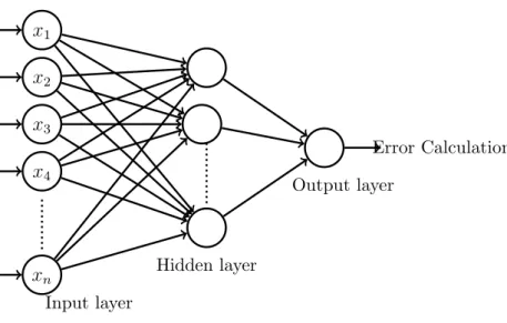
In multilayered feedforward network, neurons are organized into layers. The in-put layer is composed not of full neurons, but rather consists simply of the values in a data record, that constitutes inputs to the next layer of neurons. The next layer is called a hidden layer; there may be many hidden nodes. The final layer is the output layer, where there is one node for each class. A single forward pass through the network results in the assignment of a value to each output node, and the record is assigned to whichever classifications node had the highest value. Mul-tilayer feedforward networks are trained using the Backpropagation (BP) learning algorithm. Backpropagation training algorithm when applied to a feed-forward multilayer neural network is known as Backpropagation neural network. Func-tional signals flows in forward direction and error signals propagate in backward direction. That’s why it is Error Backpropagation or shortly backpropagation network. The activation function that can be differentiated (such as sigmoidal activation function) is chosen for hidden and output layer computational neurons. The algorithm is based on an error - correction rule. Learning is based upon mean squared error and generalized delta rule. The rule applied for weight updation is generalized delta rule [18], [6].

The algorithm defines:

1. Initialization of weights (w) and biases (b) to random small values and target (t) is fixed.

2. Forward computation: Output of each layer is y = Φ (wx×b). where w = synaptic weight, x = input and b = bias value. Output of input layer is the input of hidden layer. In this way actual output is calculated.

3. Error is calculated by the difference of target and the actual output at output layer of neuron. Error e=t−y .

(34)

Output layer Error Calculation Input layer Hidden layer x1 x2 x3 x4 xn

Figure 3.1: Multilayered Backpropagation Neural Network

4. Backward computation: Error at each layer is calculated by partial differen-tiation. For output layer error, e0 = 0.5×(dΦ (hidden)/dy(hidden))×e

and For hidden layer error,eh = (dΦ (Yinput)/dYinput)×w0ut×e0.

5. Weights and biases in each layer are updated according to the computed errors. Updated weight, wnew = wold−lr×elayer ×xlayer layer . Updated

bias, bnew =bold−lr×elayer layer where elayer is the error of the particular

layer and xlayer is the input that is fed to the layer and lr is the learning

rate.

6. Step 2 to 5 is repeated until the acceptable minimized error.

3.2.2

BP Neural Network Classifier Hybrid with PCA

Al-gorithm

Although back propagation is the most popular learning method in the neural network community, the drawbacks of it are often pointed out:

1. Very slow computing speed

2. The possibility of getting trapped in local minima.

3. More hidden nodes leads to overfitting and greater capacity of assimilating data.

(35)

3.2 Classifiers

4. The convergence obtained from backpropagation learning is very slow. 5. The convergence in backpropagation learning is not guaranteed.

3.2.3

Why SVM for cancer classification

SVMs are used for cancer classification mainly due to following two reasons: 1. SVMs have demonstrated the ability to not only correctly separate entities into appropriate classes, but also to identify instances whose established classifi-cation is not supports by the data.

2. SVM have many mathematical features that make them attractive for gene expression analysis, including their flexibility in choosing a similarity function, sparseness of solution when dealing with large data sets, the ability to handle large feature spaces, and the ability to identify outliers.

3.2.4

The SVM Classifier and Kernel Selection

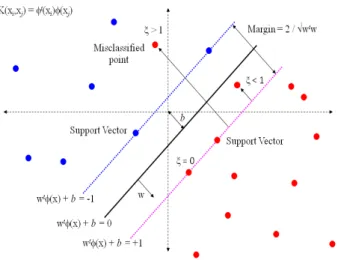
A support vector machine (SVM) [19] is a computer techniques used for the supervised learning process to analyze and recognize patterns, derived from sta-tistical learning theory developed by Vladimir N. Vapnik and Corinna Cortes in 1995. The goal of SVM is to produce a model (based on the training set) which predicts the target values of the test set making it as a non-probabilistic linear classifier. Viewing the input data as two sets of vectors in a d-dimensional space, an SVM constructs a separating hyperplane in that space, which maximizes the margin between the two classes of points. Intuitively, a good separation is achieved by the hyperplane that has the largest distance to the neighbouring data points of both classes. Larger margin or distance between these parallel hyperplanes in-dicates better generalization error of the classifier [19]. Implies that only support vectors matter; other training examples are ignorable.

The SVM is designed for binary-classification problems, assuming the data are linearly separable. Given the training data (xi, yi), i= 1,2....m, xiRn, yi{+1,−1}t

where,

(36)

Figure 3.2: SVM Classifier

xi : is the sample vector and

yi : is the class label of xi,

the separating hyperplane (w, b) is a linear discriminating function that solves the optimization problem: min w,b 1 2W ·W T subject to Yi(< W ·Xi >+b)−1≥0 (3.2) i= 1,2...m.

The minimal distance between the samples and the separating hyperplane, i.e. the margin, is 1

kWk. Data points closest to the hyperplane are called Support

Vectors. In order to relax the margin constraints for the nonlinearly separable data, the slack variables ξi are introduced into the optimization problem:

min w,b,ξ 1 2W ·W T ₊_C m X i=1 ξi subject to Yi(< W ·Xi >+b)≥1−ξi... (3.3)

ξi ≥ 0 In terms of these slack variables, the problem of finding the hyperplane

that provides the minimum number of training errors, i.e. to keep the constraint violation as small as possible. C > 0 is the penalty parameter of the error term. The problem of finding the weight vector w can be formulated as minimizing the

(37)

3.2 Classifiers following function: L(w) = 1 2kwk 2 (3.4) subject to yi(w·φ(xi) +b)≥1 (3.5)

i= 1, 2..., n. Here, b is the bias and the function, φ(x) maps the input vector to the feature vector.

Quadratic optimization algorithms can identify which training points xi are

sup-port vectors with non-zero Lagrangian multipliers αi which used to solve the

op-timization problem.

The dual formulation is given by maximizing the following: Find α1, ...., αN such that

Q(α) = n X i=1 αi− 1 2 n X i=1 n X j=1 yiyjαiαjK(xi, xj) (3.6) subject to (1) yi P αi = 0, and (2) 0 ≤ αi ≤ C∀ αi, i=1, 2,...., n where f(x) =P αiYiXTi X + b

Only a small fraction of the αi coefficients are nonzero. The corresponding

pairs of xi entries are known as support vectors and they fully define the decision

function.

SVM maps the training samples from the input space into a higher-dimensional feature space via a mapping function, called kernel function.

Furthermore,K(Xi, Xj) =XiT ·Xj is called the kernel function. There are

following four basic kernels: linear, Gaussian, RBF, Sigmoid kernels as below. Linear Kernel:

K(xi, xj) = xTi xj

Polynomial kernel:

(38)

Radial basis function kernel:

K(xi, xj) = exp(−γkxi−xjk)2

Sigmoid kernel:

K(xi, xj) = tanh(kxi·xj −δ)

Now BPNN and SVM are applied to the reduced data set to find the networks accuracy.

Many computation techniques are proposed for solving the first problem, but gives very less attention to solve other problems. The number of reduced features retrieved will be determined by cumulative energy threshold value.

3.3

Proposed Work I:

After the data set is normalizes using the following euquation, PCA is then implemented for reducing the high dimensional DNA microarray data. On the reduced data set feed forward neural network and SVM are implemented and their performance accuracies are compared.

3.3.1

Data Preprocessing and Cleaning

Filling in missing values, smoothing noisy data, identifying and removing out-liers and resolving inconsistencies.

3.3.2

Data Normalization

Data normalization is followed after data preprocessing and cleaning. Data normalization is essential to the performance of classifiers. We use Z-min-max

(39)

3.3 Proposed Work I:

normalization method. It transforms the data into the desired range [0, 1].

Xnorm = (Xm×n−min)/(max−min) (3.7)

Xnorm is the result of the normalization, xmn is the feature(gene) to be

normal-ized,max is upper bound of the gene expression value, and min is lower bound of the gene expression value.

SVM and BPNN often does not gives better accuracy for high dimension, to improve the efficiency, we proposed to apply Principal component analysis on the original data set, to obtain a reduced dataset containing possibly uncorrelated variables without any loss [5], [18]. Then the reduced data set will be applied to SVM and BPNN classifier to improve performance of the classifier.

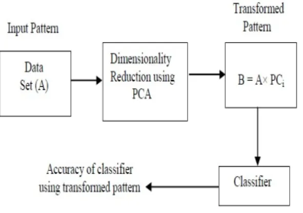
Our first contribution is to prove that PCA is able to reduce dimension of features and to provide classification competitive performance than traditional classifiers in terms of speed and predictive accuracy, and precision of convergence [20]. Hybrid approach is being proposed for reduction of features and structure mod-eling of classifiers using PCA [16], [17]. After the implementation of PCA, two classifiers such as Feed Forward Neural Network (FFNN) trained using BP algo-rithm and SVM [19] are implemented. The general procedure of the algoalgo-rithm explianed in the Figure 3.3:

Figure 3.3: PCA-SVM or PCA-BPNN classifiers for cancer data

(40)

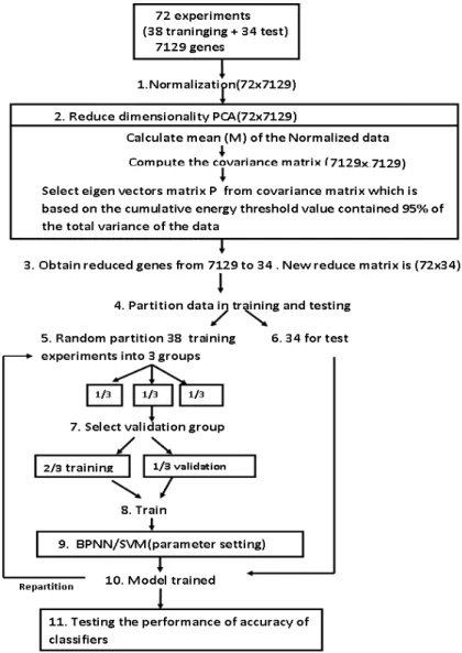
Figure 3.4: Schematic illustration of the proposed method for Leukemia cancer data

The entire data set of all 72 experiments was first Normalized (step 1) and then the dimensionality was further reduced by principal component analy-sis (PCA) to 34 PCA projections, (2) from the original 7129 expression values. Next, the 34 test experiments were set aside (6) and the 38 training experiments were randomly partitioned into 3 groups from reduced matrix (5). One of these groups was reserved for validation and the remaining 2 groups for traning (7). BPNN/SVM models were then trained using for each sample the 34 PCA values as input and the cancer category as output (9). The samples were again randomly partitioned and the entire training process repeated (10). The 34 test experiments

(41)

3.3 Proposed Work I:

were subsequently classified using all the trained models. The entire process (5-10) was repeated.

Algorithm:

The goal of PCA is to derive another matrix P matrix which will describe a linear transformation of every column in X(every training gene) in the eigenfaces sub-space, in the form: W=PX, where W are the projections of the training genes on the subspace described by the eigenfaces. The rows of P matrix represent the principal components and they are orthogonal.

The steps involved in proposed algorithm are as follows:

Data: DNA Microarray input matrix X

Result: Reduced data set

Phase-1: Apply PCA to reduce the dimension of the data set (input matrix X) Step 1: Let’s suppose we have X data matrix with m rows of samples and n columns of genes (features). aijs represent the gene values.

Step 2: To reduce redundant or missing values in matrix X we apply data nor-malization on matrix X as follows equation:

Xnorm = (Xm×n−min)/(max−min) (3.8)

Step 3: Calculate the mean M from the data set where Xi (i = 1, 2,..., m) represents the ith _{column of X and M represent the mean of genes.}

M = 1 n n X i=1 Xi (3.9)

Step 4: The genes are mean M centered by subtracting the mean value of gene from each gene vector and let Ki be defined as mean centered genes.

Ki =Xi−M (3.10)

Where i=1, 2, ..., n.

Step 5: Compute the covariance matrix SA, where A = [K1, K2... Kn]:

SA = n

X

i=1

(42)

Step 6: Calculate the Eigen Values λ1, λ2..., λn of the Covariance matrix SA, as

sorted in a decreasing order. Let the corresponding eigen vectors be denoted as

a1, a2..., an.

Step 7: Choosing components and form a feature vector by taking the eigenvec-tors that you want to keep from the list of eigenveceigenvec-tors, and forming a matrix

P[m×a] with these eigenvectors in the columns, Where a is determined based on some threshold on the eigenvalues. The cumulative energy threshold value can be calculated as: Pg i=1xi Pp i=1xi > θ (3.12)

Step 8: Derive the new data set with principal components (PC’s) by the following formula

Final Data (P C0s) = Original matrix (X) x eigenvector matrix

Phase-2: Apply SVM [19] or BPNN [18]

Step 9: Partition reduced Final data in training and testing data set. Step 10: Train BPNN and SVM model with training data and

Step 11: Test BPNN and SVM model with testing data and calculate the accu-racy.

Now BPNN and SVM applied to the reduced data set to find the networks accu-racy.

3.4

Implementation

The simulation process is carried on a machine having Intel(R) core (TM) 2 Duo processor 3.0 GHz and 3 GB of RAM. The MATLAB version used is R2012(a). The simulation was carried out with 3 microarray cancer data sets.

3.4.1

Data Sets

Data Set 1: Leukemia cancer

(43)

3.4 Implementation

Leukemia(AML) and Acute Lymphoblastic Leukemia (ALL). The complete dataset contains 25 AML and 47 ALL samples. 38 samples for training set and 34 samples for test set are chosen for simulation).

Number of Attributes: 7129

Resultant data set (after PCA): 72x34.

The data sets taken from public Kent Ridge Biomedical Data Repository with URL: http://sdmc.lit.org.sg/GEDatasets/Datasets.html. or following

URL: http://www.inf.ed.ac.uk/teaching/courses/dme/html/datasets0405.html.

Data Set 2: Ovarian cancer

Number of Instances: 216 (consist of 2 classes for distinguishing: Cancer and Normal. The complete dataset contains 121 ovarian cancer and 95 normal cancer samples. 119 samples for training set and 97 samples for test set are chosen for simulation).

Number of Attributes: 4000.

The data set taken from public Kent Ridge Biomedical Data Repository with url http:// sdmc.lit.org.sg/GEDatasets/Datasets.html.

Data Set 3: Colon cancer

Number of Instances: 62 (consist of 2 classes for distinguishing: tumor biopsies and normal biopsies . The samples consist of 36 tumor biopsies collected from tumors, and 27 normal biopsies collected from healthy part of the colons of the same patient.)

Number of Attributes: 2000.

The data sets taken from http://microarray.princeton.edu/oncology.

3.4.2

Input Parameters

We have design BPNN architecture as 72x3x1 for Leukemia cancer, 216x3x1 for Ovarian and 62x3x1 for colon cancer data set.

(44)

BPNN Paramerters: Number of nodes in hidden layer=3, learning rate=0.2, Number of iterations=1000.

SVM Parameters: C = 2, γ = 8, d = 3.

The parameters that should be optimized include penalty parameter C and the kernel function parameters such as theγ(gamma) and d for the radial basis func-tion (RBF) kernel. Generally d is set to be 2. Thus the kernel value is related to the Euclidean distance between the two samples. γ is related to the kernel width. Proper parameters setting can improve the SVM classification accuracy.

3.4.3

Performance Measures

The measure used to evaluate the performance of classifiers:

Accuracy = (correctly classified instances) / (Total no. of instances) *100%

1. Accuracy =(TP+TN) / (TP+FP+TN+FN) 2. Sensitivity = (TP/TP+FN)*100%

3. Specificity = (TN/ TN+FP) * 100%

Where, TP = true positive, TN = true negative FP = false positive, FN = false negative.

3.5

Numerical Simulation, Results and

Discus-sion

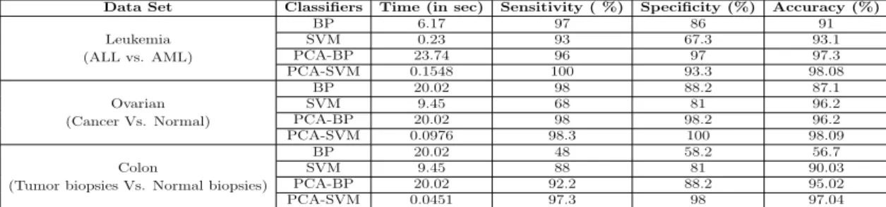
Initially simulation was carried out considering the original features and BPNN and SVM classifiers. This classification aaproach is validated by considering three other data sets i.e. Leukemia cancer, Ovarian cancer and colon cancer data. The accuracy obtained with traditional BPNN and SVM were 91% and 93.1% taking Leukemia cancer and 87.1% and 96.2% taking Ovarian cancer and 56.7% and 90.03% taking Colon cancer data respectively showing in Table 3.2 and Table 3.3. After the implementation of PCA, the data distribution across the first three principal components (PC’s) and first two principal components (PC’s) are shown

(45)

3.5 Numerical Simulation, Results and Discussion

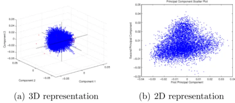
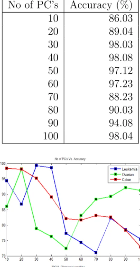
below in Figure 3.5 for Leukemia cancer data set, Figure 3.6 for Ovarian cancer data set. The classification accuracy varying with number of principal components (PC’s) showing in Table 3.1. The data distribution across the first two features showing in Figure 3.8. The Accuracy Vs. graphs were plotted for the principal component which has shown the maximum accuracy showing in Figure 3.7. The accuracy obtained with traditional BPNN and SVM were showing in Table 3.3.

(a) 3D representation (b) 2D representation

Figure 3.5: 3D and 2D Schematic representation of data across first three PC’s and two PC’s (Leukemia Cancer data set)

(a) 3D representation (b) 2D representation

Figure 3.6: 3D and 2D Schematic representation of data across first three PC’s and two PC’s (Ovarian Cancer data set)

Using PCA-based approach, the original number of features in Leukemia cancer got reduced from 7129 to 34 Latents (PC’s) (i.e. reduced by 99.03%). It covers 95% of the total variance of the data. Therefore, there is hardly any loss of information along a dimension reduction. If the first 34 PC’s are chosen, it gives best classification results. In Ovarian cancer from 4000 to 28 (i.e. reduced by 82%) and Colon cancer from 2000 to 12 Latents (i.e. reduced by 86.05%). Considering the reduced features, the accuracy obtained with PCA-BPNN and PCA-SVM were

(46)

Table 3.1: Accuracy vs. No. of PC’s using PCA-SVM (Leukemia Cancer data set) No of PC’s Accuracy (%) 10 86.03 20 89.04 30 98.03 40 98.08 50 97.12 60 97.23 70 88.23 80 90.03 90 94.08 100 98.04

Figure 3.7: Plot showing Accuracy vs. No. of PC’s using PCA

Figure 3.8: 2D Schematic representation of data across first two features (Leukemia data set)

97.3% and 98.08% for leukemia cancer and 96.2% and 98.09% for Ovarian data set and 95.02% and 97.04% for Colon cancer data set respectively.

(47)

3.6 Conclusion

Table 3.2: Classification Results: SVM Kernels

Data Set Classifiers Time (in sec) Sensitivity ( %) Specificity (%) Accuracy (%)

(ALL vs. AML) Linear 0.1548 100 93.33 96.08 Leukemia Polynomial 0.0696 100 83.33 87.08 RBF 0.1548 100 93.3 98.08 Sigmoid 0.0580 58.9 76.2 58.82 (Cancer Vs. Normal) Linear 0.1976 98.3 100 84.02 Ovarian Polynomial 0.1793 98.3 100 98.04 RBF 0.0976 80 64.1 74.02 Sigmoid 0.2818 34.4 76.9 59 (Tumor biopsies Vs. Normal biopsies)

Linear 0.0956 98.3 100 84.02 Colon Polynomial 0.0451 97.03 98 99.02 RBF 0.1146 85.2 94.4 84.8 Sigmoid 0.2318 34.4 66.9 69

Table 3.3: Classification Results: Traditional BP, SVM, PCA-BP, and PCA-SVM

Data Set Classifiers Time (in sec) Sensitivity ( %) Specificity (%) Accuracy (%)

(ALL vs. AML) BP 6.17 97 86 91 Leukemia SVM 0.23 93 67.3 93.1 PCA-BP 23.74 96 97 97.3 PCA-SVM 0.1548 100 93.3 98.08 (Cancer Vs. Normal) BP 20.02 98 88.2 87.1 Ovarian SVM 9.45 68 81 96.2 PCA-BP 20.02 98 98.2 96.2 PCA-SVM 0.0976 98.3 100 98.09 (Tumor biopsies Vs. Normal biopsies)

BP 20.02 48 58.2 56.7

Colon SVM 9.45 88 81 90.03

PCA-BP 20.02 92.2 88.2 95.02 PCA-SVM 0.0451 97.3 98 97.04

3.6

Conclusion

PCA-BP learning algorithm is designed to reduce network error between the actual output and the desired output of the network in a gradient descent man-ner. Experimental results illustrate PCA-SVM method showing better results than PCA-BPNN, traditional BPNN and SVM, in terms of speed, accuracy and complexity. The two stage approach of classification has shown promising results as they have outperformed traditional approaches. In this work the problem of cancer classification is solved successfully using PCA-SVM. If the data are con-centrated over a particular linear subspace, PCA provides a way to compress data and simplify the representation without losing much information. But if the data are concentrated over a non-linear subspace, PCA fails to work well. Work can be further extended by implementing singular value decomposition or indepen-dent component analysis for dimension reduction. Accuracy can be checked by considering some more number of objectives (such as discarded features, weight value association with accuracy etc.) which can be efficiently solved using Genetic algorithm(GA) [21] and MultiObjective Genetic algorithm (MOGA) [15].

(48)

(49)

Chapter 4

Multiobjective Genetic

Algorithm-Based Fuzzy

Clustering combining with

Support Vector Machine for

Clustering and Classification

We propose a novel method for selecting the final clustering solution from the set of Pareto-optimal solution based on majority voting among the Pareto front solutions. Non-dominated Sorting Genetic Algorithm-II (NSGA-II) based multiobjective clustering algorithm has been adopted that optimizes the cluster compactness and cluster separation simultaneously. A challenging issue in MOO is obtaining a final solution from the set of Pareto-optimal solutions. It combines the multiobjective clustering technique with support vector machine (SVM) based classifier to obtain the good performance of classifier in terms of accuracy, speci-ficity and sensitivity for classification and in terms of Silhoutte Index and ARI Index for clustering [19].

The main contributions of this article are embodied in the following five as-pects:

1. This article presents two fitness functions (fuzzy compactness and fuzzy separation) for an individual chromosome, being optimized simultaneously. 2. This approach identifies the solution i.e. the individual chromosome which

(50)

3. The multi-objective technique is first used to produce a set of non-dominated solution. The non-dominated set is then used to find some high confidence points using a fuzzy voting technique.

4. Points which have higher degree are taken as a training data in SVM classifier and remaining points as testing data.

5. An experiment is designed and is being applied this approach to three mi-croarray cancer data set. The experimental results confirm that MOGA-SVM approach gives more effective result for classification and clustering. 6. Performance of MOGA-SVM compared with other classifiers and methods

in terms of accuracy, sensitivity, specificity, Silhoutte index and ARI index.

4.1

Evolutionary Algorithms

Two most desirable features of an Evolutionary Algorithm:

• Convergence to Pareto optimal front- To improve the convergence on the Pareto fronts Multiobjective Evolutionary Algorithm (MOEA) uses non-dominated sorting algorithms.

• Maintenance of Diversity (Representation of the entire Pareto optimal front)-Increase the diversity of solutions.

4.1.1

Brief Overview of GA

Genetic algorithms (GAs) [21] [22] are popular search and optimization strate-gies guided by the principle of Darwinian evolution. Although genetic algorithms have been previously used in data clustering problems [23] [24], as earlier, most of them use a single objective to be optimized, which is hardly equally applicable to all kinds of datasets.

4.1.2

Single Objective Optimization Problem (SOOP)

An optimization problem that involves optimization of single objective is known as Single Objective Optimization Problem.

(51)

4.1 Evolutionary Algorithms

In general a single objective function can be defined as minimizing or maxi-mizing a function f(x) subject to inequality constraints g(x) ≥ 0, for all i = 1, 2...,m and equality constraints h(x) = 0, for all j = 1, 2.... p, xΩ. So, the solution minimizes or maximizes the function f(x), where x is a n-dimensional de-cision vector variablex= (x1, x2...xn) from some universe Ω. The inequality and

equality constraints must be fulfilled while optimizing (minimizing or maximizing) the objective function f(x). In SOOP, only a single optimal solution is obtained. And either the maximum or the minimum fitness value is selected as the optimal (best) solution depending upon the problem.

4.1.3

Multiobjective Optimization

Multiobjective Optimization (MOO) is a very powerful technique, used to find solutions to many real-world search and optimization problems. Many of these problems have multiple objectives, which lead to the need of obtaining a set of optimal solutions, known as effective solutions. It has been found that Multiobjective Optimization algorithm is a highly effective one for finding multiple effective solutions in a single simulation run. It means that can be optimized simultaneously.

The multiobjective optimization criterion [25] formally, can be stated as fol-lows: Find the vector x∗ = [x∗₁, x∗₂..., x∗_n]T of the decision variables that will satisfy the ’m’ inequality constraints as,

gi(x)≥0, i= 1,2, ..., m (4.1)

and the p equality constraints as,

hi(x) = 0, i= 1,2, ..., p (4.2)

and optimizes the vector function

f(x) = [f1(x), f2(x)..., fk(x)]T (4.3)

The constraints given in (4.1) and (4.2) define the feasible region F which contains all the admissible solutions. Any solution outside this region is inadmissible since

(52)

it violates one or more constraints. The vectorx∗ denotes an optimal solution in F. In the context of multiobjective optimization, the difficulty lies in the definition of optimality, since we find a situation where a single vector x∗ represents the optimum solution with respect to all the objective functions.

In a precise manner, MOPs are those problems where the goal is to optimize k objective functions simultaneously. The set of k objective functions can be either all maximize or all minimize or combination of both. The objective functions can be linear or non-linear and continuous or discrete in nature. There are a number of popular multiobjective optimization techniques. Among them, the GA based techniques such as NSGA-II, and SPEA2 [26] are very popular.

4.1.4

Brief Overview of MOGA

Multiobjecyive optimization is different from single objective optimization. In single objective optimization one attempt to obtain the best design or decision. Which is usually global maximun or global minimum depending on the optimiza-tion problem is that of minimizaoptimiza-tion or maximizaoptimiza-tion. In the case of multiple objectives there may not exist one solution which is best (global maximum or global minimum) with respect to all objectives. In a typical multiobjective op-timization problem, there exists a set of solution which are superior to the rest of solutions in the search space when all objectives are considered but are infe-rior to other solutions in the space in one or more objectives. These solutions are known as pareto optimal solutions or non-dominated solutions [27]. To solve many real-world problems, it is necessary to optimize more than one objective simulta-neously. MOGA has been introduced to optimize multiobjective problems [15]. Recently, a lot of multiobjective GAs (MOGAs) have been used by researchers for microarray cancer data. Basically, MOGA is characterized by its fitness as-signment and diversity maintenance strategy. Multiobjective genetic algorithms (MOGAs) are used in this regard in order to determine the appropriate cluster centers (modes) and the corresponding partition matrix. Non-dominated sorting GA-II (NSGA-II), which is a popular elitist MOGA, is used as the underlying optimization method. The two objective functions, i.e., the global fuzzy

(53)

compact-4.1 Evolutionary Algorithms

ness of the clusters and fuzzy separation, are optimized simultaneously. Unlike single objective optimization, which yields a single best solution, in MOO the final solution set contains a number of Pareto-optimal solutions, none of which can be dominated or further improved on any one objective without degrading another.

The single objective formulation is extended to reflect the nature of multi-objective optimization problem where there is more than one multi-objectives function which needs to be optimizing [25]. Thus there is set of solutions instead of a single solution i.e. a set of optimal solution and they are found using Pareto-optimality theory. The set of solutions obtained is based on dominance and non-dominance.

Issues in MOGA

• Fitness assignment- In each generation the non-dominated set is maintained, fitness is adjusted according to the domination of each individual.

• Density estimation- In order to encourage diversity in the population fitness is reduced for similar solutions.

4.1.5

Fast Non-Dominated Sorting

Generally non-dominated sorting is one of the main time consuming parts of multiobjective evolutionary algorithm (MOEA). So, design of fast non-dominated sorting algorithm is very necessary to improve the performance of a MOEA.

In fast dominated sorting approach, the population is sorted based on non-domination. After initializing the population, it is sorted based on non-domination in each front. The first front being completely dominant in the current population, the individuals in the second front is only dominated by the individuals of first front and the front goes on. The individuals are assigned rank (fitness) values or based on front to which they belong. Individuals of first front are assigned rank 1 and individuals in second front are assigned a value of 2 and so on. In addition to rank also a second parameter called crowding distance is calculated for every individual. Crowding distance measures how close an individual is to its neighbours. Large crowding distance will maintain a better diversity in the population. NSGA - II has been designed in such a way that the time complexity

(54)

is small, hence the non-domination process is fast.

For population size of P and number of objective function O, fast non-dominated can defined as follow

For each individual p, two entities are calculated

• Domination Count, np the number of individuals (solutions) which

domi-nates the individual p, and

• Sp, a set of solutions which the individual p dominates.

All solutions in the first non-domination front will have np = 0. Then for every

individual q in Sp, reduce the domination count by one and in doing so, if for

any individual the domination count becomes zero then we put it into separate list Q, and the second front is identified. The process is continued until all fronts are identified. The total complexity of the fast non-domination procedure isOP2_,

whereas the complexity of normal non-domination sorting is OP3_.

NSGA

The Non-dominated sorting Genetic Algorithm is a popular non-domination based genetic algorithm for multiobjective optimization. Actually NSGA is an extension of Genetic Algorithm for solving multiple objective function optimiza-tions.

Drawbacks of NSGA:

• Computational complexity,

• Lack of elitism and

• Choosing the optimal parameter value for sharing parameter σshare.

Pareto Terminology

The concept of Pareto optimality comes handy in the domain of multi