TRANSFORM USING FULL LENGTH WINDOWS
PETER L. SØNDERGAARD
Abstract. This paper extends the ecient factorization of the Gabor frame operator developed by Strohmer in [17] to the Gabor analysis/synthesis opera-tor. The factorization provides a fast method for computing the discrete Gabor transform (DGT) and several algorithms associated with it. The factorization algorithm should be used when the involved window and signal have the same length. An optimized implementation of the algorithm is freely available for download.
1. Introduction
The nite, discrete Gabor transform (DGT) of a signalf of lengthLis given by
(1) c(m, n, w) =
L−1 X
l=0
f(l, w)g(l−an)e−2πiml/M.
Here g is a window (lter prototype) that localizes the signal in time and in fre-quency. The DGT is equivalent to a Fourier modulated lter bank withM channels and decimation in timea, [2].
Ecient computation of a DGT can be done by several methods: If the windowg has short support (consists of relatively few lter taps), a lter bank based approach can be used. We shall instead focus on the case when g and f are equally long. The main advantage of the algorithm presented is its ease of use: The running time is guaranteed to be small even for long windows. This allows for the practical use of non-compactly supported windows like the Gaussian and its tight and dual windows without truncating them.
In the case when the window and signal have the same length, a factorization of the frame operator matrix was found by Zibulski and Zeevi in [19]. The method was initially developed in theL2(R)setting, and was adapted for the nite, discrete setting by Bastiaans and Geilen in [1]. They extended it to also cover the anal-ysis/synthesis operator. A simple, but not so ecient, method was developed for the Gabor analysis/synthesis operator by Prinz in [15]. Strohmer [17] improved the method and obtained the lowest known computational complexity for computing the Gabor frame operator. This paper extends Strohmer's method to also cover the Gabor analysis and synthesis operators.
The advantage of the method developed in this paper as compared to the one developed in [1], is that it works with FFTs of shorter length, and does not require multiplication by complex exponentials caused by the quasi-periodicity of the Zak transform. The two methods have the same asymptotic complexity,O(N MlogM), where M is the number of channels and N is the number of time steps. A more accurate op count is presented later in the paper.
We shall study the DGT applied to multiple signals at once. This is for instance a common subroutine in computing a multidimensional DGT. The DGT dened by (1) works on a multi-signalf ∈CL×W, whereW ∈Nis the number of signals.
2. Definitions
We shall denote the set of integers between zero and some number Lby
(2) hLi= 0, . . . , L−1.
The Discrete Fourier Transform (DFT) of a signal f ∈CL is dened by (FLf) (k) = √1 L L−1 X l=0 f(l)e−2πikl/L. (3)
We shall use the · notation in conjunction with the DFT to denote the variable
over which the transform is to be applied. To denote all elements indexed by a variable we shall use the :notation. As an example, if C ∈ CM×N then C:,1 is a
M ×1 column vector, C1,: is a 1×N row vector andC:,: is the full matrix. This
notation is commonly used in Matlab and FORTRAN programming and also in some prominent textbooks, [8].
The convolution f∗g of two functionsf, g∈CL and the involutionf∗ is given by (f∗g) (l) = L−1 X k=0 f(k)g(l−k), l∈ hLi (4) f∗(l) = f(−l), l∈ hLi. (5)
It is well known how convolution can be computed eciently using the discrete Fourier transform. We shall use a variant of this result
(f∗g∗) (l) =
√
LFL−1(FLf) (·) (FLg) (·)(l). (6)
The Poisson summation formula in the nite, discrete setting is given by
FM b−1 X k=0 g(·+kM) ! (m) = √b(FLg) (mb), (7) where g∈CL,L=M bwithb, M∈N.
A family of vectorsej,j∈ hJiof lengthLis called a frame if constants0< A≤
B exist such that
(8) Akfk2≤ J−1 X j=0 |hf, eji| 2 ≤Bkfk2, ∀f ∈CL.
The constants Aand B are called lower and upper frame bounds. IfA =B, the frame is called tight. IfJ > L, the frame is redundant (oversampled). Finite- and innite dimensional frames are described in [4].
A nite, discrete Gabor system (g, a, M)is a family of vectorsgm,n∈CL of the following form
(9) gm,n(l) =e2πilm/Mg(l−na), l∈ hLi
for m ∈ hMiand n ∈ hNiwhere L= aN and M/L ∈N. A Gabor system that
is also a frame is called a Gabor frame. The analysis operator Cg : CL 7→CM×N associated to a Gabor system(g, a, M)is the DGT given by given by (1). The Gabor synthesis operator Dγ : CM×N 7→ CL associated to a Gabor system (γ, a, M)is given by (10) f(l) = N−1 X n=0 M−1 X m=0 c(m, n)e2πiml/Mγ(l−an).
Algorithm 1 Window factorization wfac(g, a, M) (1) forr=hcik=hpi,l=hqi (2) fors=hdi (3) tmp(s)← g(r+c·(k·q−l·p+s·p·q mod d·p·q)) (4) end for (5) P hi(r, k, l,:)←dft(tmp) (6) end for (7) return Phi
In (1), (9) and (10) it must hold thatL=N a=M bfor someM, N ∈N. Addition-ally, we denec, d, p, q∈Nby c= gcd (a, M) , d= gcd (b, N), (11) p=a c = b d , q= M c = N d, (12)
where GCD denotes the greatest common divisor of two natural numbers. With these numbers, the redundancy of the transform can be written as L/(ab) =q/p, where q/p is an irreducible fraction. It holds that L = cdpq. The Gabor frame operator Sg : CL 7→ CL of a Gabor frame (g, a, M) is given by the composition of the analysis and synthesis operators Sg =DgCg. The Gabor frame operator is
important because it can be used to nd the canonical dual window gd = S−1 g g
and the canonical tight window gt=S−1/2
g gof a Gabor frame. The canonical dual
window is important because Dgd is a left inverse ofCg. This gives an easy way to
construct an inverse transform of the DGT. Similarly, then Dgt is a left inverse of
Cgt. For more information on Gabor systems and properties of the operatorsC,D
and S see [9, 6, 7].
3. The algorithm
We wish to make an ecient calculation of all the coecients of the DGT. Using (1) literally to compute all coecientsc(m, n, w)would require8M N LW ops.
To derive a faster DGT, one approach is to consider the analysis operator Cg
as a matrix, and derive a faster algorithm through unitary matrix factorizations of this matrix. This is the approach taken by [17, 16]. Unfortunately, this approach tends to introduce many permutation matrices and Kronecker product matrices. Another approach is the one taken in [1] where the Zak transform is used. This approach has the downside that values outside the fundamental domain of the Zak transform require an additional step to compute. In this paper we have chosen to derive the algorithm by directly manipulating the sums in the denition of the DGT.
To nd a more ecient algorithm than (1), the rst step is to recognize that the summation and the modulation term in (1) can be expressed as a DFT:
(13) c(m, n, w) =
√
LFLf(·, w)g(· −an)(mb).
We can improve on this because we do not need all the coecients computed by the Fourier transform appearing in (13), only everyb'th coecient. Therefore, we
Algorithm 2 Discrete Gabor transform dgt(f, g, a, M) (1) P hi=wfac(g, a, M) (2) for r=hci (3) fork=hpi,l=hqi,w=hWi (4) fors=hdi (5) tmp(s)← f(r+ (k·M+s·p·M −l·ha·amod L), w) (6) end for (7) P sitmp(k, l+w·q,·)←dft(tmp) (8) end for (9) fors=hdi (10) G←P hi(:,:, r, s) (11) F ←P sitmp(:,:, s) (12) Ctmp(:,:, s)←GT ·F (13) end for (14) for u=hqi,l=hqi,w=hWi (15) tmp←idft(Ctmp(u, l+w·q,:)) (16) fors=hdi (17) coef(r+l·c, u+s·q−l·ha modN, w) ←tmp(s) (18) end for (19) end for (20) end for (21) forn=hNi,w=hWi (22) coef(:, n, w)←dft(coef(:, n, w)) (23) end for (24) returncoef
can rewrite by the Poisson summation formula (7): c(m, n, w) = √MFM b−1 X ˜ m=0 f(·+ ˜mM, w)g(·+ ˜mM−an) ! (m) = (FMK(·, n, w)) (m), (14) where K(j, n, w) =√M b−1 X ˜ m=0 f(j+ ˜mM, w)g(j+ ˜mM−na), (15)
forj ∈ hMiandn∈ hNi. From (14) it can be seen that computing the DGT of a
signal f can be done by computingK followed by DFTs along the rst dimension ofK.
To further lower the complexity of the algorithm, we wish to express the sum-mation in (15) as a convolution.
We splitjasj =r+lcwithr∈ hci,l∈ hqiand introduceha, hM ∈Zsuch that the following is satised:
(16) c=hMM −haa.
The two integersha, hM can be found by the extended Euclid algorithm for
Using (16) and the splitting ofj we can express (15) as K(r+lc, n, w) = √M b−1 X ˜ m=0 f(r+lc+ ˜mM, w)× ×g(r+l(hMM−haa) + ˜mM−na) (17) = √M b−1 X ˜ m=0 f(r+lc+ ˜mM, w)× ×g(r+ ( ˜m+lhM)M−(n+lha)a) (18)
We substitutem˜ +lhM bym˜ andn+lha bynand get
K(r+lc, n−lha, w) = √M b−1 X ˜ m=0 f(r+lc+ ( ˜m−lhM)M, w)× ×g(r+ ˜mM−na) (19) = √ M b−1 X ˜ m=0 f(r+ ˜mM+l(c−hMM), w)× ×g(r+ ˜mM−na) (20)
We split m˜ =k+ ˜spwithk∈ hpiands˜∈ hdiand n=u+sq withu∈ hqiand
s∈ hdiand use thatM =cq,a=cpandc−hMM =−haa:
K(r+lc, u+sq−lha, w) = √M p−1 X k=0 d−1 X ˜ s=0 f(r+kM+ ˜spM−lhaa, w)× ×g(r+kM−ua+ (˜s−s)pM) (21)
After having expressed the variables j, m˜,n using the variablesr,s, ˜s,k,l, uwe have now indexed f using ˜s and g using (˜s−s). This means that we can view the summation over s˜as a convolution, which can be eciently computed using a discrete Fourier transform. Dene
Ψf r,s(k, l+wq) =Fdf(r+kM+·pM−lhaa, w), (22) Φg r,s(k, u) = √ MFdg(r+kM+·pM−ua), (23)
Using (6) we can now write (21) as
K(r+lc, u+ ˜sq−lha, w) = √d p−1 X k=0 F−1 d Ψfr,·(k, l+wq) Φgr,·(k, u) (˜s) (24) = √dFd−1 p−1 X k=0 Ψfr,·(k, l+wq) Φgr,·(k, u) ! (˜s) (25)
If we considerΨfr,sandΦgr,sas matrices for eachrands, the sum overkin the last
line can be written as matrix products. Algorithm 2 follows from this. 4. Running time
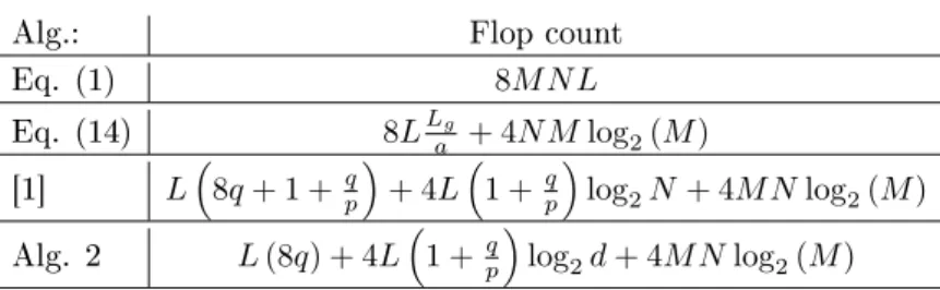
When computing the op count of the algorithm, we will assume that a complex FFT of length M can be computed using 4Mlog2M ops. A nice review of op counts for FFT algorithms is presented in [14]. Table 1 shows the op count for
Table 1. Flop counts
Alg.: Flop count
Eq. (1) 8M N L
Eq. (14) 8LLg
a + 4N Mlog2(M)
[1] L8q+ 1 + qp+ 4L1 + qplog2N+ 4M Nlog2(M) Alg. 2 L(8q) + 4L1 + qplog2d+ 4M Nlog2(M)
Flop counts for 4 dierent way of computing the DGT: By the linear algebra denition (1), by the method based on Poisson summation (14), by the method of
Bastiaans and Geilen from [1] and by Algorithm 2. The termLg denotes the
length of the window used soLg/ais the overlapping factor of the window. Note
for comparison thatlog2N = log2d+ log2q
Algorithm 2 and compares it with the denition of the DGT (1), with the algorithm for short windows using Poisson summation (14) and with the algorithm published in [1]. The algorithm by Prinz presented in [15] has the same computational com-plexity as the Poisson summation algorithm. For simplicity we assume that both the window and signal are complex valued. In the common case when bothf and g are real-valued, all the algorithms will see a 2 to 4 times speedup.
The op count for denition (1) is that of a complex matrix multiplication. All the other algorithms share the 4M Nlog2M term coming from the application of an FFT to each 'block' of coecients and only dier in how the application of the window is performed. The Poisson summation algorithm is very fast for a small overlapping factor Lg/a, but turns into an O L2
algorithm for a full length window. In this case the other algorithms have an advantage. The term L8q+ 1 + qp in the [1] algorithm comes from calculation of the needed Zak-transforms, and the4L1 +qplog2N term comes from the transform to and from
the Zak-domain. Compared to (22) and (23) this transformation uses longer FFTs. Algorithm 2 does away with the multiplication with complex exponentials in the [1] algorithm, and so the rst term reduces to L(8q).
Both the Poisson summation based algorithm and Algorithm 2 can do a DGT with L≈2000000in less than 1 second on a standard PC at the time of writing. We have not created an ecient implementation of the algorithm from [1] in C so therefore we cannot reliably time it.
5. Extensions
The algorithm just developed can also be used to calculate the synthesis operator Dγ. This is done by applying Algorithm 2 in the reverse order and inverting each
line. The only lines that are not trivially invertible are lines 10-12, which becomes 10) Γ←P hid(:,:, r, s)
(11) C←Ctmp(:,:, s) (12) P sitmp(:,:, s)←Γ·C
where the matricesP hid(:,:, r, s)should be left inverses of the matricesP hi(:,:, r, s)
for each rands.
The matrices P hid(:,:, r, s)can be computed by Algorithm 1 applied to a dual
Gabor window γ of the Gabor frame (g, a, M). It also holds that all dual Gabor windows γ of a Gabor frame (g, a, M) must satisfy that P hid(:,:, r, s) are left inverses of the matrices P hi(:,:, r, s). This criterion was reported in [11, 12].
Algorithm 3 Canonical Gabor dual window gabdual(g, a, M) (1) P hi=wfac(g, a, M) (2) for r=hci,s=hdi (3) G←P hi(:,:, r, s) (4) P hid(:,:, r, s)← G·GT−1 ·G (5) end for (6) gd=iwfac P hid, a, M (7) return gd
A special left-inverse in the Moore-Penrose inverse. Taking the pseudo-inverses of P hi(:,:, r, s)yields the factorization associated with the canonical dual window of (g, a, M), [3]. This is Algorithm 3. Taking the polar decomposition of each matrix in Φg
r,s yields a factorization of the canonical tight window (g, a, M).
For more information on these methods, as well as iterative methods for computing the canonical dual/tight windows, see [13].
6. Special cases We shall consider two special cases of the algorithm:
The rst case is integer oversampling. When the redundancy is an integer then p= 1. Because of this we see thatc=aandd=b. This gives (16) the appearance
(26) a=hMqa−haa,
indicating that hM = 0 and ha = −1 solves the equation for all a and q. The
algorithm simplies accordingly, and reduces to the well known Zak-transform al-gorithm for this case, [10].
The second case is the short time Fourier transform. In this case a =b = 1, M =N =L,c=d= 1, p= 1,q=Land as in the previous special case hM = 0
andha=−1. In this case the algorithm reduces to the very simple and well known
algorithm for computing the STFT.
7. Implementation
The reason for dening the algorithm on multi-signals, is that the multiple signals can be handled at once in the matrix product in line 12 of Algorithm 2. This is a matrix product of two matrices size q×pandp×qW, so the second matrix grows when multiple signals are involved. Doing it this way reuses the Φgr,s matrices as much as possible, and this is an advantage on standard, general purpose computers with a deep memory hierarchy, see [5, 18].
The benet of expressing Algorithm 2 in terms of loops (as opposed to using the Zak transform or matrix factorizations) is that they are easy to reorder. The presented Algorithm 2 is just one among many possible algorithms depending on in which order ther,s,kandlloops are executed. For a given platform, it is dicult a priory to estimate which ordering of the loops will turn out to be the fastest. The ordering of the loops presented in Algorithm 2 is the variant that uses the least amount of extra memory.
Implementations of the algorithms described in this paper can be found in the Linear Time Frequency Toolbox (LTFAT) available from http://ltfat.sourceforge. net. The implementations are done in both the Matlab/Octave scripting language and in C. A range of dierent variants of Algorithm 2 has been implemented and tested, and the one found to be the fastest on a small range of computers is included in the toolbox.
References
[1] M. J. Bastiaans and M. C. Geilen. On the discrete Gabor transform and the discrete Zak transform. Signal Process., 49(3):151166, 1996.
[2] H. Bölcskei, F. Hlawatsch, and H. G. Feichtinger. Equivalence of DFT lter banks and Gabor expansions. In SPIE 95, Wavelet Applications in Signal and Image Processing III, volume 2569, part I, San Diego, july 1995.
[3] O. Christensen. Frames and pseudo-inverses. J. Math. Anal. Appl., 195:401414, 1995. [4] O. Christensen. An Introduction to Frames and Riesz Bases. Birkhäuser, 2003.
[5] J. Dongarra, J. Du Croz, S. Hammarling, and I. Du. A set of level 3 basic linear algebra subprograms. ACM Trans. Math. Software, 16(1):117, 1990.
[6] H. G. Feichtinger and T. Strohmer, editors. Gabor Analysis and Algorithms. Birkhäuser, Boston, 1998.
[7] H. G. Feichtinger and T. Strohmer, editors. Advances in Gabor Analysis. Birkhäuser, 2003. [8] G. H. Golub and C. F. van Loan. Matrix computations, third edition. John Hopkins University
Press, 1996.
[9] K. Gröchenig. Foundations of Time-Frequency Analysis. Birkhäuser, 2001.
[10] A. J. E. M. Janssen. The Zak transform: a signal transform for sampled time-continuous signals. Philips Journal of Research, 43(1):2369, 1988.
[11] A. J. E. M. Janssen. On rationally oversampled Weyl-Heisenberg frames. Signal Process., pages 239245, 1995.
[12] A. J. E. M. Janssen. The duality condition for Weyl-Heisenberg frames. In Feichtinger and Strohmer [6], chapter 1, pages 3384.
[13] A. J. E. M. Janssen and P. L. Søndergaard. Iterative algorithms to approximate canonical Gabor windows: Computational aspects. J. Fourier Anal. Appl., 13(2):211241, 2007. [14] S. Johnson and M. Frigo. A Modied Split-Radix FFT With Fewer Arithmetic Operations.
IEEE Trans. Signal Process., 55(1):111, 2007.
[15] P. Prinz. Calculating the dual Gabor window for general sampling sets. IEEE Trans. Signal Process., 44(8):20782082, 1996.
[16] S. Qiu. Discrete Gabor transforms: The Gabor-gram matrix approach. J. Fourier Anal. Appl., 4(1):117, 1998.
[17] T. Strohmer. Numerical algorithms for discrete Gabor expansions. In Feichtinger and Strohmer [6], chapter 8, pages 267294.
[18] R. C. Whaley, A. Petitet, and J. Dongarra. Automated empirical optimization of software and the ATLAS project. Technical Report UT-CS-00-448, University of Tennessee, Knoxville, TN, Sept. 2000.
[19] Y. Y. Zeevi and M. Zibulski. Oversampling in the Gabor scheme. IEEE Trans. Signal Process., 41(8):26792687, 1993.