New forecasting models

NEW FORECASTING MODELS

1

1 _{The authors acknowledge the financial support of the Hong Kong University Grant Council's Competitive Earmarked}

Research Grant - B-Q976. Gang Li School of Management University of Surrey Guildford GU2 7XH United Kingdom Tel: +44 1483 686356 Fax: +44 1483 686346 Email: [email protected] Haiyan Song

School of Hotel and Tourism Management The Hong Kong Polytechnic University Hung Hom, Kowloon

Hong Kong

Tel: +852 2766 6372 Fax: +852 2362 9362

Email: [email protected]

ABSTRACT

Tourism forecasting plays an important role in tourism planning and management. Various forecasting techniques have been developed and applied to the tourism context, amongst which econometric forecasting has been winning an increasing popularity in tourism research. This paper therefore aims to introduce the latest developments of econometric forecasting approaches and their applications to tourism demand analysis. Particular emphases are placed on the time varying parameter (TVP) forecasting technique and its application to the almost ideal demand system (AIDS). The discussions in this paper fall into two main parts, in line with the two broad categories of econometric forecasting approaches: the first part refers to the single-equation forecasting techniques, focusing particularly on both long-run and short-term TVP models. The second part introduces the system-of-equations forecasting models, represented by the AIDS and its dynamic versions including the combination with the TVP technique, will be discussed one by one following the order of methodological developments.

KEYWORDS: Forecasting Models, Time Varying Parameter (TVP), Almost Ideal Demand System (AIDS)

INTRODUCTION

Considering the data availability, tourism forecasting techniques fall into two major categories: quantitative and qualitative forecasting. If little or no quantitative information is available, but sufficient qualitative knowledge exists, qualitative forecasting approaches are appropriate. When sufficient quantifiable information about the past is available and the objective numerical measurements are consistent over the historical period, quantitative forecasting should be adopted. Considering the number of published studies, quantitative forecasting dominates the tourism literature.

Quantitative forecasting methods can be further divided into two subcategories: causal and non-causal methods, depending on if there are any explanatory variables included or not in the models. Causal methods, principally the econometric models, can not only predict the trends of future tourism demand, but also interpret the causes of variations in tourism demand. Hence, causal forecasting methods can provide useful information for both policy evaluation in the public sector and strategy formulation in various tourism businesses. This paper focuses on the latest developments of econometric forecasting methods and their applications in the tourism context. A particular emphasis will be given to the TVP estimation approach applied to both single-equation and system-of-equation models.

TVP SINGLE-EQUATION MODELS

One of the assumptions behind conventional fixed-parameter econometric techniques is that the coefficients of the models are constant over the whole sample period. This implies that the economic

structure generating the data does not change over time (Judge et al, 1985). However, the changing

economic environment may induce people to react differently at various points in time, both quantitatively and qualitatively to given stimulations. To overcome the limitations of the traditional fixed-parameter models, a more advanced and flexible econometric method: the TVP model, has been developed, which allows one to understand and forecast consumer behaviour more accurately. The TVP model relaxes the restriction on the parameter constancy and takes account of the possibility of parameter changes over time. The TVP technique was initially developed in the engineering science and was recently applied to socioeconomic studies, mostly adopted in the single-equation modelling framework.

TVP Long-Run Model (TVP-LRM)

TVP models are normally specified in a state space (SS) form. SS modelling assumes that the dynamic features of the system under study are determined by the unobserved variables associated with a series of observations (Durbin and Koopman, 2001). The SS presentation allows unobserved variables to be included into, and estimated along with, the observable variables. By inferring the relevant properties of the unobserved series from the knowledge of the observations, the evolution of the system can be more precisely described and predicted. A linear SS model can be written as:

, t t t t Z y = ′

α

+

ε

ε

~ N(0,H_t), t=1,...,T (1) , 1 t t t t T

α

η

α

₊ = +

α

₁ ~ N(a₁,P₁),

η

_t ~ N(0,Q_t), (2)

where y_t is the dependent variable; Z_t is a vector of independent variables;

α

_t is an unobserved

vector called state vector;

ε

_t refers to the temporary disturbance and

η

_t the permanent disturbance,

t

ε

and

η

_t are Gaussian disturbances, which are serially independent and independent of each other at

all time points; The matrices T_t, H_t and Q_t are initially assumed to be known. Equation (1) is called

the observation equation, and Equation (2) called the state equation. In most of the economic

applications, the evolution of

α

_t is assumed to follow a multivariate random walk. i.e.,

t t

t

α

η

α

₊1 = + . This assumption is also applied in the current study. The initial value of

α

t, i.e.,

α

1,

variance of

α

₁ (Durbin and Koopman, 2001; Harvey, 1989).

The rationale behind this model is that the evolution of the concerning system over time is determined

by

α

_t according to the state equation. Meanwhile, since it is unobservable, the analysis must be based

on the observations of y_t, that is, Z_t and T_t−1 are dependent on y₁,…,y_t−1.

The definition of the state vector

α

_t for a particular model depends on its construction. Its elements

have a substantive interpretation, e.g., as a trend or seasonality. From a technical point of view, the

purpose of specifying a SS form is to “set up

α

_t in such a way that it contains all the relevant

information on the system at time t and that it does so by having as small a number of elements as

possible” (Harvey, 1989, p102).

Once a TVP model has been specified in a SS form, the Kalman filter procedure (Kalman, 1960) can be employed to calculate the optimal (minimum mean square error, MMSE) estimator of the state

vector at time t, given the information available up to time t-1. Since the Kalman filter yields

T T T T T a

α

1 | 1 +

+ = and the MMSE estimator of

α

T+1 given all the observations, the one-step-ahead

forecast can be directly produced by:

T T a Z yT 1|T T 1 _1| ~ ~ + + + = ′ (3)

where Z~_Tt+1 is the vector of one-step-ahead forecasts of explanatory variables such as the disposable

income or the consumer price index. The forecasts of these macroeconomic indicators are normally available from the national statistics office, or projected using the appropriate non-causal time-series forecasting approach.

Correspondingly, the multi-step forecasts can also be recursively generated. Full illustration of the Kalman filter technique is available from Harvey (1989).

Since the observation equation (1) is based on the classical econometric model—the static or long-run cointegration (CI) model, the TVP specification of Equation (1) is known as TVP-LRM.

TVP Error Correction Model (TVP-ECM)

Equation (1) suggests that the TVP-LRM emphases the evolution of explanatory variables and its effect on the dependent variable. Although it is useful to examine the annual demand for tourism over a long period, the dynamic changes of tourism demand in the short term are also concerned by tourism businesses. To serve this purpose, an error correction model (ECM) could be considered. Engle and Granger (1987) showed that in a system of two variables, if a long-run equilibrium relationship exists, the short-term disequilibrium relationship between the two variables can be represented by an ECM. The ECM reflects the mechanism of the short-run adjustment towards the long-run equilibrium in the system. If there are more than two variables in the system, it is possible that there will be more than one CI relationships, and correspondingly the ECM becomes a vector ECM.

The conventional fixed-parameter ECM assumes that the speed of short-run adjustment is constant over time. In the changing environment such an assumption seems to be too strict and arbitrary. In fact, “even assuming the existence of a stable long-run combination, one may find signs of instability in the

short-run adjustment mechanism” (Ramajo, 2001). Therefore, it is more realistic to specify the TVP short-run dynamics within the long-run equilibrium framework. Such a specification is termed

TVP-ECM. Compared to the classical long-run TVP model, the TVP-ECM adds one more restriction—existence of the CI relationship, and focuses on the short-term adjustment, the speeds of which vary over time.

After confirming the acceptance of a CI relationship, a TVP-ECM can be estimated. Similar to the TVP-LRM, the TVP-ECM can also be specified in a SS form.

In the case where the lag length of the differenced variables is zero, which has been proved to be appropriate in most tourism studies using annual data, the observation equation of the TVP-ECM can be written as: t t t t t t Z e v y =∆ ′ + + ∆

β

λ

ˆ₋1 (4)

where eˆ_t−1 = y_t−1−Z_t′₋₁

α

ˆ are the OLS residuals from the CI function yt =Zt′

α

+et, where

α

(without a subscript) is a fixed parameter vector. eˆ_t−1 represents the error correction mechanism.

β

_t

and

λ

_tare the TVP vectors, and v_t is the temporary disturbance term. The state equation still takes the

same form as Equation (2), and

α

_t =(

β

_t,

λ

_t)′. The estimation method is the same as that of the

TVP-LRM.

It should be noted that dummy variables can be readily incorporated into both the TVP-LRM and the TVP-ECM, in order to capture the effects of one-off events such as the Iraqi War and 9.11 terrorist attack. Since these one-off events are regarded as exogenous factors for tourism demand, it is not necessary to estimate the parameters using the TVP technique and the fixed parameters are appropriate for dummy variables in a TVP model.

Applications of TVP Models in Tourism

TVP models in both long-run and dynamic forms have been successfully applied in economic studies such as modelling and forecasting rational expectation formations, inflation, and demand for money

and other products (e.g., Bohara and Sauer, 1992; Swamy et al, 1990; and Hackl and Westlund, 1996).

However, applications of TVP models to tourism forecasting are still rare, with the following notable exceptions. Riddington (1999) utilised the TVP-LRM to analyse and forecast ski demand in Scotland. Song and Witt (2000) used the TVP-LRM to examine the demand elasticity changes over time

regarding the demand for Korean tourism by UK and USA residents. Li et al (2005a) and Song et al

(2003b) showed the superiority of the TVP-LRM to its fixed-parameter counterparts in terms of

forecasting accuracy in their studies on tourism demand in Denmark and Thailand, respectively. Li et

al (2006) examined the forecasting performance of both TVP-LRM and TVP-ECM relative to a

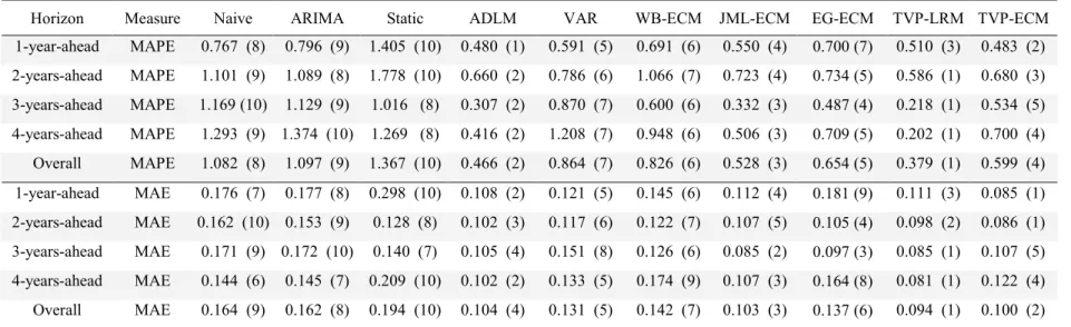
number of fixed-parameter econometric and time series models in an empirical study of UK tourism demand in some key Western European destinations. Table 1 shows that the overall performance of the TVP-LRM in terms of demand level forecasting is the best amongst all the models in the comparison. The TVP-ECM always performs above average. As far as demand growth is concerned, the TVP-LRM and TVP-ECM outperform all of their competitors. In particular, the TVP-ECM generates the most accurate one-year-ahead and two-years-ahead forecasts. The consistently superior performance of the TVP-LRM and TVP-ECM suggests that the TVP technique is an effective tool for tourism demand

Table 1 Forecasting Accuracy over Different Forecasting Horizons

Horizon Measure Naive ARIMA Static ADLM VAR WB-ECM JML-ECM EG-ECM TVP-LRM TVP-ECM

1-year-ahead MAPE 0.767 (8) 0.796 (9) 1.405 (10) 0.480 (1) 0.591 (5) 0.691 (6) 0.550 (4) 0.700 (7) 0.510 (3) 0.483 (2) 2-years-ahead MAPE 1.101 (9) 1.089 (8) 1.778 (10) 0.660 (2) 0.786 (6) 1.066 (7) 0.723 (4) 0.734 (5) 0.586 (1) 0.680 (3) 3-years-ahead MAPE 1.169 (10) 1.129 (9) 1.016 (8) 0.307 (2) 0.870 (7) 0.600 (6) 0.332 (3) 0.487 (4) 0.218 (1) 0.534 (5) 4-years-ahead MAPE 1.293 (9) 1.374 (10) 1.269 (8) 0.416 (2) 1.208 (7) 0.948 (6) 0.506 (3) 0.709 (5) 0.202 (1) 0.700 (4) Overall MAPE 1.082 (8) 1.097 (9) 1.367 (10) 0.466 (2) 0.864 (7) 0.826 (6) 0.528 (3) 0.654 (5) 0.379 (1) 0.599 (4) 1-year-ahead MAE 0.176 (7) 0.177 (8) 0.298 (10) 0.108 (2) 0.121 (5) 0.145 (6) 0.112 (4) 0.181 (9) 0.111 (3) 0.085 (1) 2-years-ahead MAE 0.162 (10) 0.153 (9) 0.128 (8) 0.102 (3) 0.117 (6) 0.122 (7) 0.107 (5) 0.105 (4) 0.098 (2) 0.086 (1) 3-years-ahead MAE 0.171 (9) 0.172 (10) 0.140 (7) 0.105 (4) 0.151 (8) 0.126 (6) 0.085 (2) 0.097 (3) 0.085 (1) 0.107 (5) 4-years-ahead MAE 0.144 (6) 0.145 (7) 0.209 (10) 0.102 (2) 0.133 (5) 0.174 (9) 0.107 (3) 0.164 (8) 0.081 (1) 0.122 (4) Overall MAE 0.164 (9) 0.162 (8) 0.194 (10) 0.104 (4) 0.131 (5) 0.142 (7) 0.103 (3) 0.137 (6) 0.094 (1) 0.100 (2) Note: The upper half of the table refers to the forecasts of level variables, and the lower differenced variables. Figures in parentheses are rankings. Naive refers to the naive

no-change model; ARIMA the autoregressive integrated moving average model; Static the static regression; ADLM autoregressive distributed lagged model; VAR the vector autoregressive model; WB-ECM the Wickens and Breusch ECM; JML the Johansen maximum likelihood ECM; EG-ECM the Engle Granger ECM. MAPE stands for mean absolute percentage errors; MAE stands for mean absolute errors.

AIDS MODELS

As addressed earlier, causal forecasting methods have advantages over the non-causal approach in terms of their abilities to interpret the reasons of tourism demand variations. Eadington and Redman (1991) noted that the single-equation econometric forecasting approach is incapable of analysing the interdependence of budget allocations to different consumer goods/services. For example, the tourism decision-making involves a choice among a group of alternative destinations. A change of price in one destination may affect tourists’ decisions on travelling to a number of alternative destinations, and also influence their expenditures in those destinations. Clearly, the single-equation methodology cannot adequately model the influence of a change in tourism price in a particular destination on the demand for travelling to all other destinations. Meanwhile, the single-equation approach cannot be used to test the symmetry and adding-up hypotheses, which are associated with the existing demand theories. The system-of-equations approach initiated by Stone (1954) overcomes the above limitations. By including a group of equations (one for each consumer good) in the system and estimating them simultaneously, this approach permits the examination of how consumers choose bundles of goods in order to maximise their utility with budget constraints. Although there are a number of system approaches available, the almost ideal demand system (AIDS), introduced by Deaton and Muellbauer (1980), has been the most commonly used method for analysing consumer behaviour. As the authors described, the AIDS model possesses the following attractive features:

· It gives an arbitrary first-order approximation to any demand system;

· It satisfies the axioms of consumers without invoking parallel linear Engel curves;

· It has a functional form which complies with known household-budget data;

· It is easy to estimate and largely avoid the need for non-linear estimation;

· The restrictions of homogeneity and symmetry can be tested though linear restrictions on fixed

parameters in the model;

· It has a flexible functional form and does not impose any a priori restrictions on the elasticities,

which means any good in the system can be either inferior or normal, and either a substitute or a

complement to the others (Fujii et al, 1985).

Although the Rotterdam and translog models also hold some of these features, neither of them contains

all these features simultaneously. Having explicit theoretical underpinnings, AIDS is more appropriate

for tourism demand analysis.

Static LAIDS

The original AIDS initialised by Deaton and Muellbauer (1980) takes a static functional form and is specified as: i j i j ij i i p x P w =

α

+

∑

γ

log +

β

log( / )+

ν

(5)

where wi is the budget share of the ith good, pi is the price of the ith good, x is total expenditure on all

goods in the system, P is the aggregate price index for the system, vi is the disturbance term,

) , 0 ( ~ i2 i N

be estimated. The aggregate price index P is defined as:

∑

+

∑∑

+ = i i j j i ij i i p p p a P log log 2 1 log log ₀

α

γ

(6)

where a₀is a parameter to be estimated. Replacing P with the Stone’s (1954) price index (P*) defined

by Equation (7), the linearly approximated AIDS is derived and termed “LAIDS”.

∑

= i i i p w P* log log (7)

The LAIDS with dummy variables can then be written as:

i k k ik j i j ij i i dum v P x p w + +      + + =

α

∑

γ

β

∑

ϕ

* log log (k=1, 2, …, m) (8)

where dum_k is a dummy variable, which handles the intervention of the exogenous shock; m is the

number of dummy variables included in the system;

ϕ

_ik is a parameter to be estimated.

Equation (8) can be re-written more compactly in the vector-matrix notation:

t t t

t z dum v

w =Π +

ϕ

+ (9)

where z_t is a q-vector of intercept, log prices and log real total expenditure variables (q=n+2); Π

and

ϕ

are (n×q) and n×mparameter matrices, respectively; Π=(

π

₁′,

π

₂′_,...

π

′_n)′, where

π

_i is a

q-vector. The LAIDS model is normally estimated by the iterated seemingly unrelated regression

(SUR) logarithm (see Zellner, 1962 for details).

To comply with the properties of demand theory, some restrictions are imposed on the parameters in

Equation (8), such as Adding-up (

∑

=

i i 1

α

,

∑

= i ij 0

γ

,

∑

=0 i i

β

and

∑

=0 i ik

ϕ

), Homogeneity (

∑

= j ij 0

γ

) and Symmetry (

γ

_ij =

γ

_ji). Subject to the satisfaction of the above restrictions, the

unrestricted LAIDS in Equation (8) can be further written as two restricted versions: the homogeneous LAIDS and the homogeneous and symmetric LAIDS. The latter is the most theoretically sound, and the further analysis and forecasting should be based on this version. However, the hypotheses of the above restrictions might be rejected by statistical tests in empirical studies. In this case, the unrestricted LAIDS or homogeneous LAIDS has to be considered.

Within the LAIDS framework, the demand elasticities can be calculated as: the expenditure

elasticity

ε

_ix =1+

β

_i/w_i, the uncompensated price elasticity

ε

_ij =−

δ

_ij +

γ

_ij/w_i −

β

_iw_j/w_i and the

compensated price elasticity

ε

_ij* =−

δ

_ij +

γ

_ij/w_i +w_j (

δ

_ij=1 for i=j;

δ

_ij=0 for i≠j). The elasticities

calculated from the LAIDS model have a stronger theoretical basis than the single-equation models. Therefore, the LAIDS model can provide more reliable information for tourism demand analysis.

Dynamic LAIDS

In the static LAIDS, which is also known as the long-run LAIDS model, it is implicitly assumed that there is no difference between consumers’ short-run and long-run behaviour, i.e. the consumers’ behaviour is always in “equilibrium”. However, in reality, habit persistence, adjustment costs, imperfect information, incorrect expectations and misinterpreted real price changes often prevent consumers from adjusting their expenditure instantly to price and income changes (Anderson and Blundell, 1983). Therefore, until full adjustment takes place consumers are “out of equilibrium”. This is one of the reasons why most static LAIDS models cannot satisfy the theoretical restrictions (Duffy, 2002). Moreover, the static LAIDS pays no attention to the statistical properties of the data and the dynamic specification arising from time series analysis. It is well known that most economic data are non-stationary, and the presence of unit roots may invalidate the asymptotic distribution of estimators.

Therefore, traditional statistics such as t, F and R2 are unreliable, and the least squares estimation of the

static LAIDS tends be spurious (Chambers, 1993; Granger and Newbold, 1974). Furthermore, the static LAIDS is unlikely to generate accurate short-run forecasts (Chambers and Nowman, 1997). However, the introduction of the CI/ECM into the LAIDS models can solve the above problems, as the error correction LAIDS—EC-LAIDS augments the long-run equilibrium relationship with a short-run adjustment mechanism.

Before examining the CI relationship, all variables concerned need to be tested for unit roots (orders of integration). The Augmented Dickey-Fuller (ADF) and Phillips-Perron (PP) statistics can be employed for this purpose. Once the orders of integration of the variables have been identified, either the Engle and Granger (1987) two-stage approach or the Johansen (1988) maximum likelihood approach can be used to test for the CI relationship among the variables in the models (Song and Witt, 2000).

Following Engle and Granger’s two-stage approach, the EC-LAIDS can be written in the following

form (Edgerton et al, 1996; Chambers and Nowman, 1997; Duffy, 2002):

t t t t t t t B L z L dum w z dum v w L A( )∆ = ( )∆ +

φ

( )∆ +Γ( ₋₁−Π ₋₁−

ϕ

₋₁)+ (10) where

∑

= + = l i i iL A I L A( ) ₁ ,

∑

= = h i i iL B L B( ) ₀ and

∑

= = s i i iL L) ₀ (

φ

φ

are matrix polynomials in the

lag operator L. l and h can be determined by using order selection techniques.

)

(wt−1−Πzt−1−

ϕ

dumt−1 is the error correction term. Given that annual data are used, most tourism

demand studies employing ECMs have shown that setting the lag length of differenced variables equal to zero is appropriate. Thus, Equation (10) can be reduced to the following form (see Durbarry and Sinclair, 2003): t t t t t t t B z dum w z dum v w = ∆ + ∆ +Γ −Π − + ∆

φ

( ₋1 ₋1

ϕ

₋1) (11)

where B is an (n×q) matrix, and

φ

is an (n×m) matrix; Γ is an (n×n)matrix. Considering the degrees of freedom and statistical significance of the estimates of the error correction terms, some empirical studies, such as Ray (1985), used a more restrictive formulation, involving only the

disequilibrium in the own budget share in each equation. In other words, Γ becomes diagonal, and

the off-diagonal terms, the estimates of which are normally insignificant, are restricted to zero. The diagonal form of Γ also implies that

Γ

ii are equal, i.e., Γ is a negative scalar.

Equation (11) reflects both long-run and short-run effects in the same model. In the short run, changes in expenditure shares depend on changes in prices, real expenditure, dummies, and the disequilibrium error in the previous period. In the long run, when all differenced terms become zero, Equation (11) is reduced to Equation (9), i.e., the system achieves its steady state.

TVP-LAIDS

As has been addressed above, TVP models have advantages over their fixed-parameter counterparts. In addition, various empirical studies have shown the superior forecasting performance of TVP models in comparison to other conventional econometric models. Meanwhile, the superiority of the AIDS model over the single-equation approach has also been evaluated. Hence, combination of the TVP technique and the AIDS/LAIDS model is likely to create both theoretically sound and more accurate forecasting methods. Consistent with the development of LAIDS specifications, the TVP-LAIDS family comprises both the long-run version—TVP-LR-LAIDS, and the short-run dynamic TVP-EC-LAIDS, depending on whether the error correction mechanism is incorporated into the LAIDS specification.

TVP-LR-LAIDS

Relaxing the fixed-parameter restriction, the unrestricted long-run LAIDS of Equation (8) can be re-written as a TVP system. It should be noted that once the estimates of the fixed-parameter LAIDS have shown the statistical significance of dummy variables, they should also be included into TVP formulations, but as exogenous variables they have fixed parameters (Ramajo, 2001). Therefore each equation of the TVP-LR-LAIDS can be written in the following one-dimension SS form:

it t i it t it z dum u w = ′

π

+

ϑ

+ uit ~ N(0,Ht), t=1,...,T ₍₁₂₎ it it it

π

ξ

π

₊1 = +

π

1 ~ N(c1,P1)_,

ξ

it ~ N(0,Qt) ₍₁₃₎

where w_it and u_it are the ith elements of vectors w_t and u_t respectively;

ϑ

_i is the ith row of

ϑ

;

ξ

_it

is a q-vector of disturbance terms.

π

_it is an unobserved state vector, and follows a multivariate

random walk. The matrices H_t and Q_tare initially assumed to be known.

Correspondingly, the whole system can be specified as: t t t t t z Π dum u w = * * +

ϑ

+ ₍₁₄₎ * * * 1 t t t

Π

ξ

Π

₊ = + ₍₁₅₎ where * , t n t I z z = ⊗ ′ _Π* ₌( _{1, 2} ,..., )′ nt t t t

π

π

π

and ( 1 , 2 ,..., ). * _{= ′} nt t t t

ξ

ξ

ξ

ξ

In homogeneity or symmetry restricted LAIDS, the restrictions (M), which are linear, can be written

as:

*

t

G

M =

Π

₍₁₆₎

where G is the coefficient matrix of the restriction.

Combining the linear restriction of Equation (16) with Equation (14) gives a new augmented measurement equation in the form:

t t t t t Z D U W = *

Π

* + + ₍₁₇₎ where _      = M w W_t t ; _      = G z Z t t * * ; _      = 0 t t dum D

ϑ

; _      = 0 t t u U . TVP-EC-LAIDS

In the pervious sections, the TVP-ECM and EC-LAIDS have been introduced. Both of these models have a particular emphasis on the short-term dynamics of the system concerned. A further combination between them generates the TVP-EC-LAIDS, which is so far the most advanced development of the LAIDS family. Specifically, the TVP-EC-LAIDS features the varying short-term adjustment towards the long-run steady state of demand.

As with Equations (12) and (13), each equation of the unrestricted TVP-EC-LAIDS can be described as the following SS form:

∆ ∆ ∆

π

θ

∆

∆

wit =(zt )′ it + i dumt +uit (18) ∆ ∆ ∆

π

ξ

π

it+1 = it + it (19) where zt∆ =(∆zt,wt−1−Πzt−1)′; ∆ it

π

is the corresponding parameter vector;

θ

_i is the ith row of

θ

;

∆ it

u is the ith item of u_t∆, the disturbance vector of the measurement equation; and

ξ

_it∆ is the

disturbance vector of the state equation.

Correspondingly, the state space form of the whole unrestricted TVP-EC-LAIDS is specified as:

∆ ∆ ∆

Π

θ

∆

∆

wt =(zt )′ t + dumt +ut * (20) * 1 ∆ ∆ ∆

Π

ξ

Π

_t+ = _t + _t (21) where 1 ( ) * _{= ⊗} ∆ _′ + ∆ t q t I z z ; =( 1 , 2 ,..., )′ ∆ ∆ ∆ ∆

π

π

π

Π

t t t nt ; ( 1 , 2 ,..., ). * ₌ ∆ ∆ ∆ _′ ∆ nt t t t

ξ

ξ

ξ

ξ

Once the unrestricted LAIDS passes the restriction tests, the homogeneity-restricted or both homogeneity and symmetry-restricted version of TVP-LR-LAIDS and TVP-EC-LAIDS can be estimated using the Kalman filter algorithm, and forecasts can be generated correspondingly.

Estimations of the single-equation TVP models, the static and dynamic (fixed-parameter) LAIDS, as well as the single-equation estimation of TVP-LAIDS models (i.e., each equation of the system is estimated separately), can all be carried out using the computing program Eviews 5.0.The system estimation of the TVP-LR-LAIDS and TVP-EC-LAIDS can be performed by the SAS 8.02 matrix programming language IML.

Applications of LAIDS to Tourism Forecasting

Although the LAIDS models have been employed widely in food demand modelling, applications in the field of tourism demand are still limited. A detailed review of the LAIDS related to tourism can be

found in Li et al (2005b). All of these LAIDS applications analysed allocations of tourists’ expenditure

in a group of destinations, with only one exception, Fujii et al (1985), who investigated tourists’

expenditure on different consumer goods in a particular destination. Most of the LAIDS studies in the

tourism context adopted the original static version, while Durbarry and Sinclair (2003) and Li et al

(2005a) specified the EC-LAIDS models to examine the dynamics of tourists’ consumption behaviour.

The empirical study of Li et al (2005a) examined UK outbound tourism demand in Western Europe.

The five major destinations in this area, Spain, France, Greece, Italy and Portugal, are the focuses of this study, with the other seventeen countries aggregated into a single group. Each of the six destination countries/group is regarded as an aggregated tourism product, purchased by UK visitors. The empirical results show that tourism demand by UK residents is most sensitive to price changes in Greece and least sensitive to price changes in Italy. The cross-price elasticities indicate that France and Spain, Italy and Portugal, and France and Greece are likely to be substitutes in the minds of UK tourists. With regard to forecasting performance, the EC-LAIDS always outperforms the static LAIDS, and in general the EC-LAIDS is over 40% more accurate than the static LAIDS.

Li et al (2006a) further developed the TVP-LR-LAIDS and TVP-EC-LAIDS to analyse the evolutions of demand elasticities over time and to examine their forecasting performance. Figure 1 shows the estimates of compensated own-price elasticities in the unrestricted TVP-LR-LAIDS models. These graphs exhibit different evolution patterns of the price elasticity. Relatively large fluctuations which occurred in the early 1980s are associated with the global economic recession during this period. Since the mid 1980s, the sensitivity of tourism demand for France, Greece and Italy to their price changes has become relatively stable, while the opposite phenomena can be observed in the cases of demand for Portugal and Spain tourism, with the influence of the Gulf War in the early 1990s being evident. As far as the forecasting performance is concerned, the unrestricted TVP-LR-LAIDS and TVP-EC-LAIDS outperform all of the other fixed-parameter counterparts in the overall evaluation of demand level forecasts. It suggests that the more advanced forecasting techniques contribute to the improvements of forecasting accuracy, and therefore should be applied more broadly in future tourism studies.

-1.3 -1.2 -1.1 -1.0 -0.9 -0.8 80 82 84 86 88 90 92 94 96 98 00 a. France -.8 -.7 -.6 -.5 -.4 -.3 -.2 -.1 .0 .1 80 82 84 86 88 90 92 94 96 98 00 b. Greece -3.0 -2.5 -2.0 -1.5 -1.0 -0.5 0.0 80 82 84 86 88 90 92 94 96 98 00 c. Italy -1.55 -1.50 -1.45 -1.40 -1.35 -1.30 -1.25 -1.20 80 82 84 86 88 90 92 94 96 98 00 d. Portugal -1.9 -1.8 -1.7 -1.6 -1.5 -1.4 -1.3 80 82 84 86 88 90 92 94 96 98 00 e. Spain Year Yea

r

Year Year Year * ii ε * ii ε * ii ε * ii ε * ii ε

Figure 1 Kalman Filter Estimates of Compensated Own-Price Elasticities (

ε

_ii*) in the Unrestricted

SUMMARY

This paper has introduced some of the latest developments of econometric approaches in tourism forecasting. The error correction mechanism and the TVP forecasting technique have been incorporated in both single-equation and system of equations (represented by LAIDS) frameworks. The empirical evidence shows that more advanced forecasting methods are likely to generate more accurate forecasts of tourism demand. Further developments and applications of econometric forecasting approaches should be therefore encouraged.

It should be noted that the above models are suitable where the annual tourism demand is concerned. In other words, their model specifications accommodate annual data well, but do not consider the seasonal patterns of tourism demand. In practice, shorter-term forecasts, such as monthly or quarterly forecasts, are of more interests to tourism businesses in the private sector. It has been observed that the seasonality tended to be featured in short-term tourism demand in most destinations and tourism industries. To meet the need for seasonal tourism forecasting, further developments of econometric forecasting methods should pay more attention to the seasonal patterns of tourism demand, and incorporate seasonal components in the TVP single-equation or TVP-LAIDS specifications. Considering the merits of the TVP technique, the various seasonality-augmented TVP models are likely to generate accurate forecasts of short-term demand for tourism.

REFERENCES

Anderson, G. and R. Blundell (1983). Testing Restrictions in a Flexible Dynamic Demand System: An Application to Consumers’ Expenditure in Canada. Review of Economic Studies, 50: 397-410.

Bohara, A. K. and C. Sauer (1992). Competing Macro-hypotheses in the United States: A Kalman Filtering Approach, Applied Economics, 24: 389-399.

Chambers, M. J. (1993). Consumers’ Demand in the Long Run: Some Evidence from UK Data. Applied Economics, 25: 727-733.

Chambers, M. J. and K. B. Nowman (1997). Forecasting with the Almost Ideal Demand System: Evidence from Some Alternative Dynamic Specifications, Applied Economics, 29: 935-943.

Deaton, A. S. and J. Muellbauer (1980). An Almost Ideal Demand System, American Economic Review, 70: 312-326. Duffy, M. (2002). Advertising and Food, Drink and Tobacco Consumption in the United Kingdom: A Dynamic Demand

System, Agricultural Economics, 1637: 1-20.

Durbarry, R. and M. T. Sinclair (2003). Market Shares Analysis: The Case of French Tourism Demand, Annals of Tourism Research, 30: 927-941.

Durbin, J. and S. J. Koopman (2001). Time Series Analysis by State Space Methods, Oxford University Press: New York.

Eadington, W. R. and M. Redman (1991). Economics and Tourism. Annals of Tourism Research, 18: 41-56.

Edgerton, D. L., B. Assarsson, A. Hummelmose, I. P. Laurila, K. Rickertsen and P. H. Vale (1996). The Econometrics of Demand Systems with Applications to Food Demand in the Nordic Countries, Kluwer Academic Publishers: London. Engle, R. F. and C. W. J. Granger (1987). Cointegration and Error Correction: Representation, Estimation and Testing,

Econometrica, 55: 251-276.

Fujii, E., M. Khaled and J. Mark (1985). An Almost Ideal Demand System for Visitor Expenditures, Journal of Transport Economics and Policy, 19: 161-171.

Granger, C. W. J. and P. Newbold (1974). Spurious Regressions in Econometrics. Journal of Econometrics, 2: 111-120. Hackl, P. and A. H. Westlund (1996). Demand for International Telecommunication: Time-Varying Price Elasticity, Journal

of Econometrics, 70: 243-160.

Harvey, A. C. (1989). Forecasting, Structural Time Series Models and the Kalman Filter. Cambridge University Press:

Cambridge.

Johansen, S. (1988). A Statistical Analysis of Cointegration Vectors. Journal of Economic Dynamics and Control, 12:

231-254.

Judge, G. G., W. E. Griffiths, R. Carter-Hill, H. Lütkepohl, and T. C. Lee (1985). The Theory and Practice of Econometrics, Second Edition, Wiley: New York.

Kalman, R. E. (1960). A New Approach to Linear Filtering and Prediction Problems, Transitions ASME, Journal of Basic Engineering, 82: 35-45.

Lanza, A. P. Temple and G. Urga (2003). The Implications of Tourism Specialisation in the Long Run: An Econometric

Analysis for 13 OECD Economies. _{Tourism Management, 24: 315-321.}

Li, G., H. Song and S. F. Witt (2005a). Forecasting Tourism Demand Using Econometric Models, in D. Buhalis et al. (eds) Tourism Dynamics, challenges and Tools: Present and Future Issues, Elsevier: Oxford, pp219-228.

Li, G., H. Song and S. F. Witt (2005b). Recent Development in Econometric Modeling and Forecasting. Journal of Travel Research, 44: 82-99.

Li, G., H. Song and S. F. Witt (2006a). Time Varying Parameter and Fixed Parameter Linear AIDS: An Application to Tourism Demand Forecasting. International Journal of Forecasting, 22: 57-71.

Li, G., K. Wong, H. Song and S. F. Witt (2006b). Tourism Demand Forecasting: A Time Varying Parameter Error Correction Model. Journal of Travel Research, 45:175-185.

Ramajo, J. (2001). Time-Varying Parameter Error Correction Models: The Demand for Money in Venezuela, 1983.I-1994.IV, Applied Economics, 33, 771-782.

Ray, R. (1985). Specification and Time Series Estimation of Dynamic Gorman Polar Form Demand Systems, European Economic Review, 27: 357-374.

Riddington, G. L. (1999). Forecasting Ski Demand: Comparing Learning Curve and Varying Parameter Coefficient Aroaches, Journal of Forecasting, 18: 205-214.

Song, H. and S. F. Witt (2000). Tourism Demand Modelling and Forecasting: Modern Econometric Aroaches, Pergamon: Oxford.

Song, H., S. F. Witt and T. C. Jensen (2003). Tourism Forecasting: Accuracy of Alternative Econometric Models, International Journal of Forecasting, 19: 123-141.

Stone, J. R. N. (1954). Linear Expenditure Systems and Demand Analysis: An Application to the Pattern of British Demand, Economic Journal, 64: 511-527.

Swamy, P. A. V. B., A. B. Kennickell and P. von zur Muechien (1990). Comparing Forecasts from Fixed and Variable Coefficient Models: The Case of Money Demand, International Journal of Forecasting, 6: 469-477.

Zellner, A. (1962). An Efficient Method of Estimating Seemingly Unrelated Regressions and Test for Aggregation Bias, Journal of the American Statistical Association, 57: 348-368.