University of Windsor University of Windsor
Scholarship at UWindsor
Scholarship at UWindsor
Major Papers Theses, Dissertations, and Major Papers
2018
Application of SuperLearner Algorithm on Prostate Cancer Data
Application of SuperLearner Algorithm on Prostate Cancer Data
Ebo Essilfie-AmoahFollow this and additional works at: https://scholar.uwindsor.ca/major-papers Recommended Citation
Recommended Citation
Essilfie-Amoah, Ebo, "Application of SuperLearner Algorithm on Prostate Cancer Data" (2018). Major Papers. 62.
https://scholar.uwindsor.ca/major-papers/62
This Major Research Paper is brought to you for free and open access by the Theses, Dissertations, and Major Papers at Scholarship at UWindsor. It has been accepted for inclusion in Major Papers by an authorized
APPLICATION OF SUPERLEARNER
ALGORITHM ON
PROSTATE CANCER DATA
by
Ebo Essilfie-Amoah
A Major Research Paper
Submitted to the Faculty of Graduate Studies
through the Department of Mathematics and Statistics
in Partial Fulfillment of the Requirements for
the Degree of Master of Science at the
University of Windsor
Windsor, Ontario, Canada
c
APPLICATION OF SUPERLEARNER ALGORITHM
ON PROSTATE CANCER DATA
by
Ebo Essilfie-Amoah
APPROVED BY:
—————————————————————–
M. Hlynka
Department of Mathematics and Statistics
—————————————————————–
A. Hussein, Advisor
Department of Mathematics and Statistics
Author’s Declaration of Originality
I hereby declare that I am the sole author of this major Paper and that no part of this major paper has been published or submitted for publication.
I certify that to the best of my knowledge, my major paper does not infringe upon anyone’s copyright nor violate any proprietary rights and that any ideas, techniques, quo-tations, or any other material from the work of other people included in my major paper, published or otherwise, are fully acknowledged in accordance with the standard referencing practices. Furthermore, to the extent that I have included copyrighted materials that surpass the bounds of fair dealing within the meaning of the Canada Copyright Act, I certify that I have obtained a written permission of the copyright owner(s) to include such materials in my major paper and have included copies of such copyright clearances to my appendix.
I declare that this is a true copy of my major paper, including any final revisions, as approved by committee and the Graduate Studies Office, and that this major paper has not been submitted for a higher degree to any other University or Institution. I authorize University of Windsor, Ontario Canada to lend this Major Paper to other institutions or individuals for the purpose of academic work.
Abstract
The objective of this major paper is to apply an ensemble method known as the SuperLearner algorithm to find the best ten gene expressions that can predict a high PSA (¿7) versus low PSA in prostate Cancer patients. We try to formulate techniques such the penalized logistic regressions, random forest and cross-validation in a way that is consistent with the formulation of the SupeLearner algorithm. To discover a patch of ten genes that can predict well the PDA level, we sample random patches of 10 genes from a pool of almost 47,000 genes and apply the superlearner algorithm to compute a cross-validated AUC. Consequently we choose groups of ten genes that have AUC exceeding 0.65. This exercise shows that many un-classified genes are correlated with high PSA.
Acknowledgments
I thank the Almighty God for His protection and security which I can not even purchased. I am especially indebted to Dr. Hussein, my suprevisor, my teacher and mentor. He has taught me more than I could ever give him credit for here. He has shown me, by his example, what a good person should be.
I would like to thank Dr. Myron Hlynka for being my department reader. He taught me the basic knowledge of stochastic processes and regression analysis, which helped me build a solid foundation for further studies in Statistics.
I am grateful to all faculty and staff members,as well as the graduate students in the Department of Mathematics and Statistics at the University of Windsor, with whom I have had the pleasure to work during this program.Each of them has provided me extensive personal and professional guidance and taught me a great deal about life in general. Nobody has been more important to me in the pursuit of this career than the members of my family. I would like to thank my parents, whose love and guidance are with me in whatever I pursue. They are my ultimate role models. Most importantly, I wish to thank my loving and supportive wife, Deines, and my two wonderful children, Albert and Junior, who provide unending inspiration.
Contents
Author’s Declaration of Originality iii
Abstract iv
Acknowledgments v
List of Figures ix
List of Tables ix
1 The SuperLearner Algorithm 1
1.1 Background . . . 1
1.2 The SuperLearner and other relevant methods . . . 3
1.3 Logistic regression with Lasso penalty . . . 7
1.3.1 Tree-based Methods . . . 9
1.3.2 The SuperLearner Algorithm . . . 14
2 Illustrating the use of the superlearner on PSA data 19 2.1 Description of the prostate cancer data sets . . . 19
3 Conclusions and Future Directions 36
3.1 Summary of the Results . . . 36
Bibliography 38
List of Figures
2.1 Word cloud for all the genes in the data base . . . 23
2.2 The first 100 most frequent genes (all the genes) . . . 24
2.3 Generate the Word cloud . . . 33
2.4 plot of frequencies of the first 10 frequent genes . . . 34
List of Tables
Chapter 1
The SuperLearner Algorithm
1.1
Background
One of the most common supervised statistical learning methodologies deals with classifica-tion of multi-category variables based on a given set of independent variables (known also as covariates or features). Historically, the logistic regression approach is a standard statistical technique addressing such classification problems. However, logistic regression models tend to over-fit the learning sample when the number pof features, or input variables, largely ex-ceeds the numbern of samples. This is referred to as the smalln large psetting, commonly found in biomedical problems. An example of such is when one desires to correlate between disease incidence and the expressions of a large number of genes based on microarray data. Apart from the logistic regression, there is also a number of methodologies in supervised statistical learning such as regression-tree-based approaches and neural networks[2]
the classes at hand). It is therefore quite difficult to make a subjective choice of which model to pick. This has led to the idea of model ensembles. Ensemble methods are approaches for pooling models together to produce one that could probably beat all of the individual model predictions. There are many ways to ensemble models and among those are the classical random forests, Bayesian model averaging and the more recent stacking approach called the superlearner algorithm [1,3,4].
Ensemble methods have been in existence for long time and therefore it is very difficult to trace when they began. The idea of deploying multiple models has been in use since 1990s. Breiman and Stehman conducted research in 1980s, where they found out that predictions made by the best single classifier are inferior to predictions made by the combination of a set of classifiers. It was concluded that predictions made by more classifiers most often give better and accurate result than made by a single classifier. In general, the phrase “Ensemble Methods” refers to building a large number of somewhat independent predictive models and then combining them by voting or averaging to yield very high performance [7]. Common types of ensemble learning are Bagging, Boosting and Random Forest all of which have the objective of improving performance in different ways. Also both Bagging and Random Forests were developed to overcome variance and bias issues.
The objective of this paper is to use a prostate cancer data set to illustrate the use of the SuperLearner algorithm in classification of a binary variable.
1.2
The SuperLearner and other relevant methods
Before proceeding to any of the learning algorithms that are used on the prostate data in the applications chapter, we first introduce several important general frameworks. For in-stance, many learning algorithms share the approach of cross-validation. Cross-validation as well as the learning algorithms that use them, can be viewed as formulas or procedures or even models that take the data as their input and output estimators of desired quan-tities. There are often two issues to deal with in building an estimator: the procedure of building the estimator itself and that of assessing its performance. These two procedures often share a fundamental tool known as loss function and its expectation which is known as risk function. Often, in building estimators (formulas or algorithms or models (M)), we maximize or minimize some sort of gain or loss function. Let us take an example of a binary classification problem. Letyi be the outcomes and xi be a vector of covariates (features) for
the ith observation, so that the data set is Dn ={(yi, xi), i= 1, ..., n}.We will use the short
hand y and x to denote the vectors of responses and that of features, respectively. One of the common models is the logistic regression model whose aim is to predict probability of success p = P(y = 1|x) for a new subject given its covariates. The algorithm takes simply the Dn and maximizes a gain function of the form
L(y,Ψ(x, β)) = N X i=1 h yi(β0+βTxi)−log(1 +e(β Tx i))i.
That is, it obtains an estimate of a vector of parameters ˆβ =argmaxβL(y,Ψ(x, β)). Notice
parameters. The function can also be nonparametric such as mean regressions using splines. The next step of the algorithm is to produce the predicted value for y given its features which is ˆp = ˆE[y|x] = 1
1+e(−βxˆ ) or even to give directly a predicted value of the response for a given set of features, ˆy = 1 if ˆp > a and ˆy = 0 otherwise, where a is a probability threshold. Therefore, we have used a loss function to obtain a target parameter, which could be y for a new subject (hence, prediction) or p ( probability of success for a new subject). Now the cross-validation operation can kick in as a method to assess the performance of the algorithm. That is, to answer the question of how good is ˆy or ˆp. For such assessment to be unbiased, one should not useDn which was used to build the model,M. So for that purpose,
and if we are lucky, we will have a test data set Dm of size m that was not used in building
the modelM. Therefore, we will be able to estimate some sort of loss or gain measure aimed at measuring the performance of our model M. Let us take the example of the logistic regression when the target parameter ispand so a natural loss is the quadratic loss function
L(y,pˆ(x)) = (ˆy−pˆ)2. Thus, the risk or the expected loss in using the model M to predictp
for a new subject isR =E[L(y, p(x))] which can be estimated by averaging over the test data (assuming the test data are independent realizations). That is, ˆR =Pm
i=11/mL(yi,pˆ(xi)).
Another possible loss function is the missclassification errorL(y,pˆ(x)) =I(y6= ˆy) where ˆyis decided by thresholding the ˆp(x) as above. Also here, the risk can be estimated from the new testing data by averaging this function over the training observationsPm
i=1 1
mI(yi 6= ˆyi). Yet
another gain function is the area under the Receiver Operating Characteristic curve (ROC), measured by AUC(“area under the curve“). Higher values of the AUC correspond to better performance of the model in classifying subjects correctly to the binary classes.
in which cross-validation is required. One is when building the model itself requires the knowledge of a nuisance parameter (such as tuning parameter in the penalized regression models like lasso) or when one does not have test data to compute the loss function for assessing the performance of the model built on the training data. In such cases, one can still use cross-validation to estimate quantities of interest such as expectations of loss functions and or tuning parameters. Below is a generic V −f old cross-validation procedure based on a loss function L(y,Ψ(x)).
Algorithm 1: Generic v−f old cross-validation
step1: DivideDnrandomly intoD1, ..., DV, assuming that every partition hasn/V, an integer
sample size.
step2: For v = 1, ..., V,
Fit the given algorithm, M, using Dn−Dv, i.e., all the data but the vth partition and
call M−v the estimated model obtained by using the D−v data set.
Compute the desired risk by averaging the loss function over the data partition Dv.
That is ˆ Rv = X (yi,xi)∈Dv 1 n/V L(yi, ˆ ΨM−v(xi)).
Here we are using the notation ΨˆM−v to indicate the target quantity (or parameter )
estimated by using the model M−v.
step3: Compute the final cross-validated loss as
ˆ R= V X v=1 1 V ˆ Rv
If a cross validation procedure sets V = n, then it is called leave-one-out (LOO). The LOO has been already in use in the survey literature under the name Jack-Knife, as one of the methods to obtain variances of finite population estimators. The cross-validation technique is not limited to just computing estimated versions of a loss function, but it can be used to generate cross-validated predicted values of the response itself, which is a key to many ensemble methods such as the superlearner algorithm.
In the next few sections we briefly describe some of the algorithms that we will use along with the superlearner algorithm.
1.3
Logistic regression with Lasso penalty
For more in depth treatment of the logistic regression with lasso penalty and its use as a classification method one can refer to [2]. We report a simple lasso logistic regression returning the predicted probabilities for a given fixed tuning parameter and one which uses v-fold cross-validation to choose optimal value for the tuning parameter based on AUC or misclassification error.
Algorith 2 (The logistic regression algorithm):
Step1: Given a data set Dn and a tuning parameter, α, compute
ˆ β =argmaxβ N X i=1 h yi(β0+βTxi)−log(1 +e(β Tx i))i+α p X j=1 |βj|.
step2: Return the model as the function acting on a vector of features, x = (x1, ..., xp) and
returning a vector of estimated probabilities
ˆ
Ψ(x) = ˆp= ˆp(x) 1 1 +e−βxˆ
Algorith 3 (V −f old cross-validated logistic regression with lasso penalty and using AUC and missclassification error to choose the tuning parameter):
Step1: Divide the data Dn into D1, ..., DV disjoint and exhaustive subsets with n/V
observa-tions in each. Make a grid of tuning parameters α >0. step2: For each α,
do:
for each v = 1, ..., V :
pass the pair of objects α and D−v =Dn−Dv to Algorithm 2and obtain Ψ(ˆ x).
Compute the predicted probabilities from the data Dv as
ˆ
Ψ(xi) = ˆp= ˆp(xi) =
1 1 +e−βxˆ i
For a sequence of cutoff points t ∈(0,1) compute yˆi = 1 if pˆi > t andyˆi = 0 otherwise
for all i such that yi ∈Dv.
Compute Sensitivity(t) = F(t) = X i:yi∈Dv I(yi = 1,yˆi = 1)/(n/V) and 1−Specif icity(t) = 1−G(t) = 1− X i:yi∈Dv I(yi = 0,yˆi = 0)/(n/V) .
Compute the misclassification error as mis(α, v) =P
i:yi∈DvI(yi 6= ˆyi)/n.
end for:
Compute the average AUC and the average misclassification error over v = 1, ..., V. end do:
Choose the optimal αCV as the one that leads to the model with the highest AUC or
the least misclassification error.
step3: Return the model with the best αCV as
ˆ
Ψ(x) = ˆp= ˆp(x) 1 1 +e(−βxˆ )
with coefficients computed from algorithm 2 by using the αCV and the entire data Dn.
1.3.1
Tree-based Methods
Here we limit ourself to the case of binary classification trees. The idea in such trees is to use binary splits based on some or all of the features. Explained in words, one would start by minimizing a loss function for all possible pairs of a feature and a cutoff point (also known as split point), (xs, c) for s = 1, ..., p and finding the pair that, for example,
minimizes a loss function computed on the two subsets that result from the split of the data by the pair. For instance, we split the data Dn into two subsets D1 = {(yi, xi) : xis ≤ c}
the two nodes are daughters of whatever node they descended from. Once two nodes are obtained, a loss function is calculated on the data in each and the total loss is computed as
L(y,Ψ(x);Dn) =L1(y,Ψ(x);D1)+L2(y,Ψ(x);D2). Finally, the pair of (xs, c) that minimizes
the above loss is chosen as the splitting pair and the same procedure is repeated for each node until a prespecified stopping criteria is met. Such criteria could be reaching a prespecified maximum number of nodes or a minimum number of observations per node. At the end of this construction, the sample space Rp of the vector x= (x1, ..., xp) will be partitioned into
regions N1, ..., NK corresponding to the K terminal nodes in the final tree.
There are many loss functions that can be used to decide the splits. For instance, in regression trees where the y is a continuous variable, a loss function such as the squared or absolute loss can be an appropriate measure to use, while ifyis a binary or class variable, then measures such AUC or missclassification error can be maximized or minimized, respectively. Generally, in classification trees, loss functions are usually based on node impurity statistics. These are statistics that measure the heterogeneity in nodes by computing observed class membership for the data in the node concerned. For instance, a node is pure if all the yi in
that node belong to one class and it has maximum impurity when equal proportions of the
yi belong to each of the classes in consideration within that node.
An example of node impurity measure is the Gini index defined as
Gm = K X k=1 ˆ Pmk(1−Pˆmk)
for themthnode in a given tree. This index measures total variance across thek classes and such interpretation is evident for the case of binary response variable (i.e., when k = 2). In
fact, when k = 2, then
Gm = ˆpm0(1−pˆm0) + ˆpm1(1−pˆm1 = 2ˆpm1(1−pˆm1)
which is exactly twice the variance of the Bernoulli variable, y estimated from the data in the mth node. Thus, the loss used to build the tree is basically
L(y,Ψ(ˆ x) = 2ˆp(1−pˆ)
where the Ψ(.) here is the model which is simply the classification tree itself. To fix the idea and see how, for example, the Gini index is in fact a loss function based on the tree, suppose we have a tree with K terminal nodes and let Ψ(.) be a vector of indicator functions,
Ψ(x) = (Ψ1(x), ...,ΨK(x)) = (I(x∈N1), ..., I(x∈NK))
where Nk is the partition of the sample space of x corresponding to the kth terminal node
of the tree.
Now clearly, the Gini index of the kth node for the binary case can be redefined as
L(y,Ψk(x)) = 2ˆpk(1−pˆk) where ˆ pk = n X i=1 yiΨk(xi) Pn i=1Ψk(xi) .
An alternative to the Gini index is the cross-entropy, given by Dm =− K X k=1 ˆ PmklogPˆmk.
A tree can be pruned (penalized) by exploring all possible subtrees and choosing the one that minimizes a penalized loss. Any of the loss functions above can be penalized by a term
α|Ψ| where α is a tuning parameter (a penalty parameter) and |Ψ| is the size of the tree (i.e., number of terminal nodes). Notice here that we denote the tree itself by Ψ, because the function Ψ(.) that we have defined above essentially represents the tree model.
Next, we will quote the classification tree algorithm as well as the random forest al-gorithm, before proceeding to the superlearner. Here we will use notational approach of Steingrimsson et al (2018), JASA
Algorithm 4 ( Binary classification tree):
For a given data set Dn, a loss function L(y,Ψ(x)), and a stopping criteria, define as
the current node the node that consists of all the observations in the data and do:
a. In the current node, identify all possible pairs(xs, c) of a feature and a split point such
that the data in the current node, is split into two parts by xs ≤c and xs > c so that
b. Select the pair (xs, c) of covariate and a split point that minimizes the given loss
func-tion computed by using the data in the parent node and divide this parent node into two mutually exclusive daughter nodes (subsets of data).
c. Check if the stopping criteria has been met for all of the current terminal nodes in the tree; if met, then return the treeΨand exit. Otherwise, set the node that is not meeting the criteria as the current parent node and repeat (b)-(c)
Algorithm 5 ( Random forest [James et al (2013) An Introduction to Statistical learning]):
Given a data set Dn, a loss function, two integers m, B, and a stopping criteria, do the
following: For b= 1, ..., B, Do:
a. Select a bootstrap sample of size n from the data
b. Grow a random forest treeΨb based on the bootstrap sample by applyingAlgorithm 4
in which step (b) is done only form randomly selected variables among thepcovariates. c. Return the tree Ψb.
end do:
Compute the target quantity (such as predicted probabilities of the event of interest or the estimated loss function) by averaging it over the tree Ψb;b = 1, ..., B.
The algorithm above is a typical example of an ensemble, as we are using a large number of trees and averaging out their predictions. The next topic is related to this idea and describes a recently proposed ensemble algorithm known as the superlearner.
1.3.2
The SuperLearner Algorithm
Stacked generalization is an ensemble method that allows researchers to combine several different prediction algorithms into one [8]. Since its introduction in the early 1990s, the
method has evolved several times into its current form known as the SuperLearner.
In stacking, multiple layers of machine learning models are placed one over another where each of the models passes their predictions to the model in the layer above it and the top layer model takes decisions based on the outputs of the models in layers below it [8].
In the early 1990s, Wolpert developed a way to combine several machine learning algo-rithms with the goal of increasing predictive accuracy. He termed the approach as stacked generalizations, which later became known as stacking[8]. Later on, Breiman demonstrated how stacking can be used to improve the predictive accuracy in a regression context,and showed that imposing certain constraints on the higher-level model improved predictive per-formance[1].
More recently, van der Laan and colleagues proved that stacking possesses certain ideal theoretical properties and defined the superlearner algorithm. In particular, under reason-able constraints, Super Learner is guaranteed to perform asymptotically as well as the best performing algorithm included in the candidate set of algorithms. [7].
The Super Learner combines predictions from several methods by using V-fold cross-validation and minimizing a user-specified loss function, such as prediction error, negative-log-likelihood, or rank loss[6].
The algorithm is quite simple and it generally operates as follows. Given the covariates of a new observation, x, a target parameter to be predicted, Ψ(x), and a library of algorithms with K members each designed to produce ˆΨ(x), compute the superlearner prediction as a
linear combination of the individual predictions, ˆΨ1(x), ...,ΨˆK(x) as follows: ˆ ΨSL(x) = K X l=1 ˆ αΨˆl(x)
where ˆα are computed in an optimal way using V-fold cross-validation.
Let us assume that we are dealing with a case of predicting the class probabilities for a binary classification situation. That is, what we are predicting is the probabilitypi =P(yi =
1|xi) so that our target parameter is Ψ(xi) = ˆpi. The computation of the optimal α in the
Algorithm 6 ( V-fold CV for computing the superlearner coefficients):
Given training data Dn, a library of K algorithms, Ψ1(.), ...,ΨK(.) that input x and
out-put a prediction of a target parameter, Ψˆl(x), do the following:
a. Partition Dn into V subsets, D1, ..., DV with equal number of observations n/V.
b. For each v = 1, ..., V, let D−v =Dn
Dv be the entire data save the vth subset.
For l= 1, ..., K build the lth algorithm using the data D−v and use such an algorithm
on the data in the subset Dv to obtain predictions{Ψˆl(xi)} for xi ∈Dv. Store these K
predictions for each of then/V observations in theDv data in a smalln/V ×K matrix.
c. Stack the V matrices into a big one, Z, with all the n×K predictions. Consider the data(y, z)as new data set withK independent variables andn observations. Note that each algorithm represents a variable.
d. Use constrained ordinary least squares (COLS) to obtain αˆl for l = 1, ..., K based on
this pseudo data of (yi, zi) for i = 1, ..., n where the zi = (zi1, ..., ziK) is a vector of
cross-validated predictions from the K algorithms trained on data excluding the Dv
that contains (yi, xi). That is,
ˆ α=argmaxα n X yi− K X αlzil !2
Chapter 2
Illustrating the use of the
superlearner on PSA data
2.1
Description of the prostate cancer data sets
Prostate cancer is the most common malignancy (other than skin cancer) diagnosed in men[5]. Prostate cancer is a disease defined by the abnormal growth of cells. These abnormal cells can proliferate in an uncontrolled way and, if left untreated, form tumors which may spread to other parts of the body. Prostate cancer has the potential to grow and spread quickly, but for most men, it is a relatively slow growing disease[5]. According to Ministry of Health And Long Term Care in Canada,Of every 100 men, about 10 will be diagnosed with prostate cancer during their lifetime,and 3 of the 100 will die from the disease[5].
A PSA value of > 4.0 ug/L has often been defined in the literature as abnormal and is frequently used as a cut-point as indicated by the Ministry of Health And Long Term Care.
use of age-related PSA cut-points, rather than using >4 ug/L for all.
The table below shows suggested age-specific ranges. In our analysis we will set a binary Table 2.1: Age-related normal PSA cut-points
Age Range (years) Serum PSA Concentration(ug/L)
40-49 <2.5
50-59 <3.5
60-69 <4.5
70-79 <6.5
Source: Oesterling JE et al. JAMA 1993; 270:860
cutoff point of PSA >7 and use the resulting classification variable as our main response. The data sets we use here are two: the Cambridge and the Stockholm data sets. Together, the two data sets contain observation on 212 men. Variables such as PSA values, age, Gleason scores as well as survival times are recorded. In addition, expressions for over 40k genes are also available for this group. This makes the current data a high-dimensional data. Our objectives from the current analysis is to find if there is a group of 10 genes whose expressions could be used to classify high versus low PSA after controlling for the effect of age. In the following, we perform the analysis using common R packages.
2.2
Analysis
Loading the required Rpackages
##Load the required libraries
library(ggplot2) library(tidyr) library(devtools)
library(dplyr) library(party) library(survival) library(SuperLearner) library(data.table) library(glmnet) library(randomForestSRC)
Below we manipulate the data sets inside the prostatecamcap and prostateStockholm R packages and combine them in one big data frame that contains gene expressions and patient demographics. We also remove genes with missing names.
library(prostateCancerCamcap)
data(camcap,package = ’prostateCancerCamcap’)
pd_camcap <- tbl_df(pData(camcap))
fd_camcap <- tbl_df(fData(camcap)) fd_camcap=fd_camcap%>%
mutate(Gene=replace(Symbol,Symbol %in% c("","NA"),NA))%>% filter(Gene != "NA")
pd_stockholm <- tbl_df(pData(stockholm)) fd_stockholm <- tbl_df(fData(stockholm))
fd_stockholm=fd_stockholm%>%
mutate(Gene=replace(Symbol,Symbol %in% c("","NA"),NA))%>% filter(Gene != "NA") exp_stockholm =tbl_df(data.frame(ID =
as.character(featureNames(stockholm)),exprs(stockholm)))
Next, we store all the gene expressions for later use .. There are more than 40k genes.
genescam=fd_camcap%>%select(Gene)%>%unique() genesstock=fd_stockholm%>%select(Gene)%>%unique() genes0=genescam%>%inner_join(genesstock)
genes=genes0%>%mutate(Gene=droplevels(Gene))
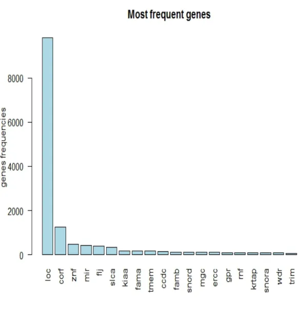
We made a word cloud of the prefixes of the names of the genes. The word cloud shows that LOC and CORF are the most common gene prefixes. The LOC prefix means that the gene’s functions are unknown. So the LOC is a sort of place holding until more informative name can be found. So, practically we are looking for a needle in a hey stack.
Figure 2.2: The first 100 most frequent genes (all the genes)
Here we start the main algorithm by creating training and test data indices. The total sample of individuals in the two sets after removing individuals with missing PSA or age is 212. We designate 80% to training data set and the remaining to validation (test).
We sample 10 genes randomly from the pool of all genes in the data base, then pull out their expression data and then clean out repeated expressions (from different probes of the same gene), by choosing only the most variable one based on IQR statistic.
genes=genes0%>%sample_n(10, replace=FALSE)%>%select(Gene) probes <- fd_camcap %>% filter(Gene %in% genes$Gene) %>%
select(ID) %>% unique %>% as.matrix %>% as.character
data<- exp_camcap %>% filter(ID %in% probes) %>% tidyr::gather(geo_accession,Expression,-ID)
summary_stats <- data %>% group_by(ID) %>%
summarise(mean=mean(Expression,na.rm=TRUE),sd=sd(Expression,na.rm=TRUE), iqr=IQR(Expression,na.rm=TRUE))
data <- left_join(data,summary_stats) %>% mutate(Z = (Expression - mean) / sd)
mostVarProbes <- left_join(summary_stats,fd) %>% arrange(Symbol,desc(iqr)) %>%
distinct(Symbol,.keep_all=TRUE) %>%
select(ID) %>% as.matrix %>% as.character
data <- left_join(data, pd_camcap)
Remove the auxiliary variables used such as the IQR, and z-scores. Then extract only age, PSA variables and the gene expression variables. Also, we classify the PSA level into above and below 7 (high and low).
data=data%>%select(-Z,-mean,-sd,-iqr,-ID)%>% tidyr::spread(Symbol,Expression) data2=data%>%select(PSA,Age,names(data[,16:25]))%>% mutate(Age=as.numeric(as.character(Age)), PSA=as.numeric(as.character(PSA)))%>% na.omit() data2cam=data2%>%mutate(PSAcp=ifelse(PSA>7,1,0))%>%select(-Age)
Next we do the same as above for the Stockholm data
###########Here starts same as above for Stockholm data probes <- fd_stockholm %>% filter(Gene %in% genes$Gene)
data<- exp_stockholm %>% filter(ID %in% probes) %>% tidyr::gather(geo_accession,Expression,-ID)
summary_stats <- data %>% group_by(ID) %>% summarise(mean=mean(Expression,na.rm=TRUE),
sd=sd(Expression,na.rm=TRUE),iqr=IQR(Expression,na.rm=TRUE))
data <- left_join(data,summary_stats) %>% mutate(Z = (Expression - mean) / sd)
mostVarProbes <- left_join(summary_stats,fd) %>% arrange(Symbol,desc(iqr)) %>%
distinct(Symbol,.keep_all=TRUE) %>%
select(ID) %>% as.matrix %>% as.character
data <- filter(data, ID %in% mostVarProbes)
data <- left_join(data, select(fd_stockholm, ID, Symbol)) data <- left_join(data, pd_stockholm)
tidyr::spread(Symbol,Expression)
data2=data%>%select(PSA,names(data[,13:22]))%>%
mutate(PSA=as.numeric(as.character(PSA)))%>%na.omit()
data2stock=data2%>%mutate(PSAcp=ifelse(PSA>7,1,0))
We join the data sets into one dataset and print first few rows
data22
# A tabble: 213 x 12
PSA PHB2 OSBP CGA APBB3 TG SCCPDH
<dbl> <dbl> <dbl> <dbl> <dbl> <dbl> <dbl> 1 28 9.68 10.1 6.57 8.94 6.05 8.26 2 99 9.62 9.55 6.44 9.84 5.94 9.01 3 75.2 9.65 10.0 6.75 9.27 6.19 8.78 4 215 9.77 10.2 6.56 9.66 6.09 8.27 5 18.6 8.98 9.15 6.84 8.96 6.17 8.30 6 200 9.62 10.6 6.61 9.63 5.94 8.04 7 60 9.52 10.9 6.46 9.67 6.08 8.57 8 48.6 9.27 10.1 6.80 9.40 5.93 8.62 9 282 9.33 9.94 6.33 9.36 6.18 8.31 10 250 9.38 10.5 6.48 8.88 6.38 8.05
ERCC-00017‘ LOC100132658 LOC642367 LOC727878 PSAcp <dbl> <dbl> <dbl> <dbl> <dbl> 6.12 8.02 8.71 6.22 1 6.07 7.57 7.74 6.10 1 5.95 8.12 8.04 6.40 1 6.10 7.58 7.93 6.36 1 5.91 8.02 7.80 6.28 1 6.21 8.48 7.58 6.19 1 6.06 8.34 7.57 6.25 1 6.08 7.83 7.85 6.27 1 6.24 8.33 8.27 6.38 1 6.28 7.34 8.56 6.31 1
# ... with 203 more rows
Take the index of the training data and create the response and covariates for the two sets. We then build the superlearner on the training data and compute the AUC on the validation set.
train_obs = trainindex
data3=data22%>%select(-PSA,-PSAcp) X_train = data3[train_obs, ]
outcome_bin = data22$PSAcp
Y_train = outcome_bin[train_obs] Y_holdout = outcome_bin[-train_obs]
We now modify the ridge and lasso regressions that are used as two of the possible algorithms
in the library of the superlearner so that these two algorithms use only V = 4 fold CV when
choosing the penalty tuning parameter and we limit the number of the grid of tuning parameters to nlambda= 10. This is simply a modification of the wrappers of the glmnet that superlearner uses internally.
SL.glmnet.lasso = function(...) {
SL.glmnet(..., nfolds = 4,nlambda=10) }
SL.glmnet.ridge = function(...) {
SL.glmnet(..., nfolds = 4,nlambda=10, alpha = 0) }
library(SuperLearner)
SL.library <- c("SL.mean", "SL.glmnet.lasso",
Next we run the main SL algorithm using lasso, ridge, usual logistic regression, simple average, and random forest as our base library of algorithms.
sl<- SuperLearner(Y = Y_train, X = X_train, SL.library = SL.library, method = "method.AUC", family = binomial()) sl Risk Coef SL.mean_All 0.6672714 0.1285674 SL.glmnet.lasso_All 0.6627362 0.1285674 SL.randomForest_All 0.5283447 0.5801448 SL.glmnet.ridge_All 0.6119426 0.1627204 SL.glm_All 0.5439153 0.0000000 >
The output shows values of the cross-validated AUCs for each algorithm as well as the optimal
α values. It is clear that the weights sum to one and the simple logistic regression algorithm has
zero weight. The highest weight of 58% goes to the random forest, followed by ridge regression. Here, we use the holdout data (test data set) to compute the AUC for the superlearner algorithm
were chosen.
pred = predict(sl, X_holdout, onlySL = T)
pred_rocr = ROCR::prediction(pred$pred, Y_holdout) auc = ROCR::performance(pred_rocr, measure = "auc",
x.measure = "cutoff")@y.values[[1]] auc
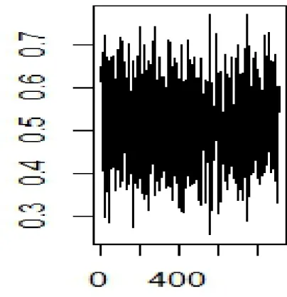
aucv[i]=auc
genesstore[i,]=transpose(genes)
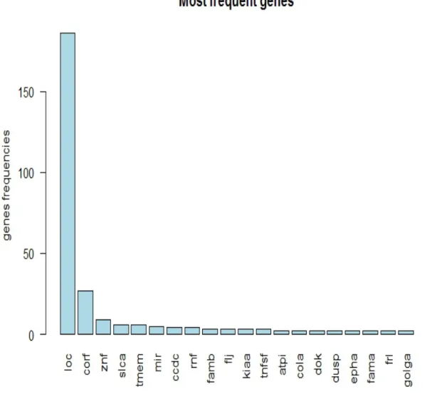
The above operation is then repeated for 2000 times and every time the 10 genes selected for the analysis and the resulting AUC are stored. Finally, below is a plot of the AUCs versus indices of the gene groups. Using the plot, we can see the patches of 10 genes that have the highest AUCs. We set a threshold of 0.8 and above for an AUC to be considered high. The resulting groups of gene from this criteria are then stored and their word cloud plotted.
Figure 2.3: Generate the Word cloud
The above word cloud clearly shows that again genes with prefixes Loc and Corf and znf are the three most important genes in the data that could be used to explain high PSA. The znf family appeared in some literature as correlated with PSA.
Figure 2.5: plot of AUC Vs Sample Number vs Sample Number.jpeg
Chapter 3
Conclusions and Future Directions
3.1
Summary of the Results
In this MSc research project, we tried to illustrate the use of the superlearner algorithm of van de Laan et al[7] to classify 212 men with prostate cancer into two groups: a group with PSA less than 7 and group with PSA higher than 7. The age was used as covariate to adjust for and the classification ability of groups of 10 gene expressions randomly selected from a data base of over 47, 000 gene expressions was explored. The data was split into training (80% ) and a test data sets. The operation of choosing 10 genes randomly from the pool, extracting their expression values, running a superlearner algorithm on the training data and building a superlearner model that can predict AUC was repeated about 1000 times. The superlearner algorithm is an ensemble method that combines the predictions from several supervised learning algorithms. We chose the logistic regression, lasso and ridge versions of logistic regression, a random forest and a simple mean model as the methods to be ensembled. The algorithm was then applied to the test data and an AUC was estimated for every run of
this gene mining operation. Finally, the AUCs of the 1000 groups of 10 genes were examined to find those with AUCs exceeding 0.7 and this collection of gene names were reported in a word cloud.
Unfortunately, we have found that most of those genes had prefix LOC, meaning that they are not well known. We do not know if some these genes are interesting and really related to PSA or can serve as a proxy for high PSA. There are a few shortcomings of this type of exercise: (1) given the large number of genes whose expression data are available and given that most of genes are likely not related to PSA, sampling 10 at time may not be sufficient to capture a representative picture of the pool of genes, (2) given the small size of this data, dividing it into training and testing sets could have reduced the power of the approach, (3) the number of ensembled algorithms is too small.
Therefore, in the future, one may want to pool more observations from different studies to increase the sample size. Also, the number of genes samples should be increased substantially even at the cost of making the problem a high-dimensional one whereby (p >> n) and then deploy more learners that are designed for such situations (e.g., random forest, neural networks and similar algorithms).
This exercise, which we have accomplished in this major paper, was just to explore the possibility of applying superlearner on publicly available prostate cancer data. The more interesting undertaking would be that of using the superlearner learning about the survival of the PCa patients, and not so much about the PSA levels.
Bibliography
[1] L. Breiman.Stacked regressions.Machine Learning ,45:5-32,2001.
[2] G. James,D. Witten,T.Hastie and R.Tibshirani.An Introduction to Statistical Learning. Springer, New York,2013.
[3] E.LeDell. Statistician and Machine Learning Scientist ,H2o.ai
[4] E.LeDell, M. Petersen, and M. van der Laan. Computationally efficient confidence in-tervals for cross-validated area under the ROC curve estimates .Electronic journal of statistics , 9(1), 1583-1607,2015.
[5] J.E. Oesterling ,S.S. Jacobsen ,C.G. Chute,H.A. Guess and C.J.Girman.Serum prostate specific antigen in a community-based population of healthy men:Establishment of age-specific ranges . JAMA ,270(7):860-4,1993 .
[6] E.C. Polley ,E.LeDell ,M.Van der Laan, C.Kennedy . Super Learner in Prediction .URL https://CRAN.R-project.org/package=SuperLearner. R package version. 2.0-22,2016.
[7] J.A.Steingrimsson ,L.Diao and R.L.Strawderman.Censoring Unbiased Regression Trees and Ensembles .Rochester, New York,2018.
[8] M.J. van der Laan,E.C. Polley, and A.E.Hubbard. Super Learner.
Statistical Applications of Genetics and Molecular Biology, 6,
article 25.
http://www.degruyter.com/view/j/sagmb.2007.6.issue-1/sagmb.2007.6.1.1309/sagmb.2007.6.1.1309.xml,2007.
Vita Auctoris
Ebo Essilfie-Amoah was born in Ghana, West Africa. He attended the University of Cape Coast, obtaining a BSc.Honours in Mathematics Dip. in Education, post Degree Diploma in Actuarial Science University of Waterloo(2008) and Master in Business Administration, University of Phoenix, USA (2010) . He is currently a candidate for the M.Sc.in Statistics from the University of Windsor.