www.geosci-model-dev.net/3/565/2010/ doi:10.5194/gmd-3-565-2010
© Author(s) 2010. CC Attribution 3.0 License.
Geoscientific
Model Development
Implementation and evaluation of a new methane model within a
dynamic global vegetation model: LPJ-WHyMe v1.3.1
R. Wania1,*, I. Ross2,**, and I. C. Prentice3,***
1Department of Earth Sciences, University of Bristol, Wills Memorial Building, Queen’s Road, Bristol, BS8 1RJ, UK 2School of Geographical Sciences, University of Bristol, University Road, Bristol BS8 1SS, UK
3QUEST, Department of Earth Sciences, University of Bristol, Wills Memorial Building, Queen’s Road, Bristol, BS8 1RJ, UK *now at: School of Earth and Ocean Sciences, University of Victoria, P.O. Box 3055 STN CSC, Victoria, BC, V8W 3V6,
Canada
**now at: Mathematics and Statistics, University of Victoria, P.O. Box 3060 STN CSC, Victoria, British Columbia V8W 3R4,
Canada
***now at: Department of Biological Sciences, Macquarie University, Sydney, NSW 2109, Australia
Received: 8 December 2009 – Published in Geosci. Model Dev. Discuss.: 15 January 2010 Revised: 15 September 2010 – Accepted: 6 October 2010 – Published: 27 October 2010
Abstract. For the first time, a model that simulates methane emissions from northern peatlands is incorporated directly into a dynamic global vegetation model. The model, LPJ-WHyMe (LPJ Wetland Hydrology and Methane), was pre-viously modified in order to simulate peatland hydrology, permafrost dynamics and peatland vegetation. LPJ-WHyMe simulates methane emissions using a mechanistic approach, although the use of some empirical relationships and param-eters is unavoidable. The model simulates methane produc-tion, three pathways of methane transport (diffusion, plant-mediated transport and ebullition) and methane oxidation. A sensitivity test was conducted to identify the most important factors influencing methane emissions, followed by a param-eter fitting exercise to find the best combination of paramparam-eter values for individual sites and over all sites. A comparison of model results to observations from seven sites resulted in normalised root mean square errors (NRMSE) of 0.40 to 1.15 when using the best site parameter combinations and 0.68 to 1.42 when using the best overall parameter combination.
1 Introduction
Wetlands are the largest individual source of methane (CH4)
emissions and contribute 100–231 Tg CH4a−1 to a global
budget of 582 Tg CH4a−1 (Denman et al., 2007).
Peat-lands are one type of wetland that occurs mainly in boreal
Correspondence to: R. Wania ([email protected])
and arctic regions, covering an area of approximately 3.0– 3.2×10⁶km2 north of 40◦N (Matthews and Fung, 1987; Aselman and Crutzen, 1989), but can also be found in tropi-cal areas such as the Amazon, Indonesia or in tropitropi-cal alpine regions (L¨ahteenoja et al., 2009; Page et al., 2010; Buy-taert et al., 2006). The common characteristic of peatlands is that they accumulate dead organic matter to a depth of at least 30 cm (Maltby and Immirzi, 1993). Zhuang et al. (2004) summarised the recent literature and found that emis-sion estimates for the pan-arctic region from eleven studies ranged from 31 to 106 Tg CH4a−1. A recent inverse
mod-elling study allocated only 33±18 Tg CH4a−1of total global
emissions to northern wetlands1(Chen and Prinn, 2006). Even though present-day methane emissions from north-ern wetlands contribute only about 5–18% of global an-nual, natural and anthropogenic, methane emissions (this estimate is based on northern wetland CH4 emissions by
Zhuang et al., 2004, and global CH4 emissions found in
Denman et al., 2007) their relative contribution may in-crease under future climate change that will inin-crease tem-perature and precipitation in the high latitude regions faster and more than in other regions on Earth (Meehl et al., 2007; Christensen et al., 2007). However, the processes that un-derlie methane emissions are complex and depend on vari-ables such as inundation, vegetation composition, and soil temperature. These variables interact with each other, and
1Although peatlands are the dominant form of wetland in boreal
vegetation, temperature and precipitation changes in the fu-ture may have a positive feedback on wetland methane emis-sions if the peatland gets warmer but stays wet or becomes wetter (Johansson et al., 2006) or a negative feedback if the peatland gets drier (Moore and Knowles, 1990; Moore and Dalva, 1993).
Methane emissions to the atmosphere result from a bal-ance between CH4production and CH4oxidation. Methane
is produced by methanogens which are obligate anaerobic archaea, which means that they require oxygen-free envi-ronments (Vogels et al., 1988; Whitman et al., 1992). The three most important factors influencing the level of activity of methanogens and therefore CH4production rates are the
degree of anoxia, the temperature, as microbes increase their activity level up to a threshold temperature after which the activity level declines again (Svensson, 1984), and the avail-ability of suitable carbonaceous substrate that can be utilised. Once CH4 is produced, it can be transported to the
atmo-sphere via diffusion through the peat pore water, it can be transported through the gas-filled pore spaces (aerenchyma) of vascular plants or it can be released abruptly in the form of bubbles.
Before methane escapes to the atmosphere, it may be oxi-dised by methanotrophic bacteria that utilise CH4as a carbon
and energy source (Hanson and Hanson, 1996). In peatlands, methanotrophs are aerobic bacteria and their activity there-fore depends on the amount of oxygen available in the peat. Oxygen can either diffuse into the peat pore water from the surface (Benstead and Lloyd, 1996) or it can be transported to the tips of the roots of vascular plants, leading to high CH4
oxidation rates (Str¨om et al., 2005). It is crucial to account for both oxygen transport mechanisms when modelling CH4
oxidation.
In order to study methane emissions from northern peat-lands, a process-based modelling approach that takes account of interactions between vegetation, hydrology, soil thermal regime and methane-related processes is needed. In the past, methane models have been developed to estimate methane emissions from global wetlands (Cao et al., 1996; Walter and Heimann, 2000; Zhuang et al., 2004), but these mod-els did not include the dynamic interactions between hydrol-ogy, soil temperature, vegetation and methane processes. A review of previous methane models can be found in Wania (2007). Here, we describe a new methane model that is in-tegrated into a dynamic global vegetation model and which takes the interactions mentioned above into account. The aim of this study is to show how LPJ-WHyMe reproduces ob-served data when simulating CH4emissions, without the use
of site-specific input data. We discuss the uncertainties that arise and the difficulties of modelling CH4emissions.
2 Model description 2.1 LPJ-WHyMe
LPJ-WHyMe v1.3.1 is a development of the Lund-Potsdam-Jena Dynamic Global Vegetation Model (LPJ) originally de-scribed by Sitch et al. (2003) and Gerten et al. (2004). LPJ is a process-based model that simulates plant physiology, car-bon allocation, decomposition and hydrological fluxes. Veg-etation is defined by plant functional types (PFTs) that group plants with similar traits. Each PFT is described by allocating specific parameters that distinguish one PFT from another. PFTs thus occupy different environmental niches defined by bioclimatic limits and physiological optima and compete for resources such as light and water. This competition deter-mines the simulated vegetation composition.
LPJ-WHyMe stands for LPJ-Wetland Hydroglogy and Methane emissions and was originally described in Wania (2007). LPJ-WHyMe is a further development of LPJ-WHy, which dealt with the introduction of permafrost and peat-lands into LPJ (Wania et al., 2009a). Implementing peatpeat-lands in LPJ-WHy required the addition of two new PFTs (flood-tolerant C3graminoids and Sphagnum mosses) to the already
existing ten PFTs, the introduction of inundation stress for non-peatland PFTs, a slow-down in decomposition under in-undation and the addition of a root exudates pool (Wania et al., 2009b). The model code is archived as supplementary material.
2.2 Methane model structure
The addition of a methane model did not require any changes to the rest of the model as the development of LPJ-WHy was targeted towards later inclusion of a methane model. A sep-arate subroutine containing the methane model was simply added to the program. All of the input variables required to drive the methane model were already available. This feature distinguishes LPJ-WHyMe from other methane mod-elling approaches, where output from vegetation models that took no account of changes in vegetation due to inundation were used to drive methane models, neglecting the poten-tial effects of changes in vegetation composition, reduction in net primary production and the deceleration of decompo-sition (e.g. Cao et al., 1996; Walter et al., 2001).
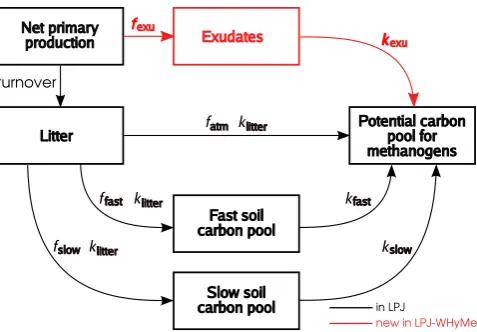
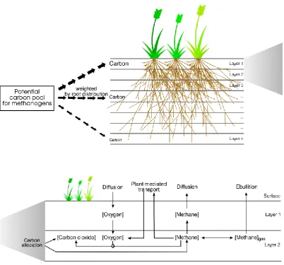
The basic concept of the methane model in LPJ-WHyMe is that a “potential carbon pool for methanogens” is created (Fig. 1). This “potential carbon pool for methanogens” is distributed over all soil layers, weighted by the root distri-bution (Fig. 2, top). This carbon is then split into CO2and
CH4(Fig. 2, bottom). Based on the amount of CH4
avail-able in each layer, the dissolved CH4concentration and the
gaseous CH4 fraction are calculated. Part of the CH4 is
to the atmosphere either by diffusion or through plant tis-sue (aerenchyma), which is also treated as a diffusive flux. Gaseous CH4 can escape to the atmosphere by ebullition.
The sum of ebullition, diffusion and plant-mediated transport represents the total CH4flux from the soil to the atmosphere.
2.2.1 Potential carbon pool for methanogens
The carbon pool available for methanogenic archaea consists mainly of root exudates and easily degradable plant material, and to a much lesser extent material from the decomposition of more recalcitrant organic matter (Chanton et al., 1995). A root exudates pool was introduced into LPJ-WHy (Wania et al., 2009b) as a very labile carbon pool with a fast turnover ratekexu. The exudates pool is directly linked to net primary
production, with a fixed fraction,fexu, of net primary
pro-duction being diverted into the exudates pool at each time step, which in this case is monthly. LPJ-WHyMe follows the same time step scheme as LPJ (Sitch et al., 2003), i.e. the time step varies between daily and yearly depending on the process. LPJ-WHyMe models the decomposition of above-and belowground litter, at rateklitter, and of the fast and the slow soil carbon pools, at rateskfast andkslow, respectively (Fig. 1). Decomposition rates are a function of soil tempera-ture (RT), which follows Lloyd and Taylor (1994) and of soil moisture content (Rmoist) via empirically fitted relationships (Wania et al., 2009b, Sect. 2.3):
k=k10RTRmoist, (1)
wherekrepresents the turnover rates for exudates, litter, and the fast and slow carbon pools, andk10 the respective de-composition rates at 10◦C (Table 1). The moisture response,
Rmoist, is chosen so that the decomposition rate is reduced under inundation and its value was determined by a param-eter fitting exercise (Table 4). The carbon resulting from this decomposition is classified as heterotrophic respiration in LPJ, but in LPJ-WHyMe, we treat this carbon differently at peatland and non-peatland sites. At non-peatland sites the pool behaves in exactly the same way as in LPJ and is im-mediately added to the atmospheric carbon dioxide flux. For peatland sites, the decomposed carbon is put into the poten-tial carbon pool available to methanogens.
2.2.2 Root distribution
Carbon from the potential carbon pool for methanogens is allocated to each soil layer according to the root biomass distribution. For the hydrology processes in LPJ-WHyMe it was sufficient to split the root biomass between acrotelm and catotelm (Ingram, 1978), but for modelling the carbon cycle within the soil, a more detailed root distribution is required to allocate carbon to each 0.1 m thick soil layer, and also to estimate the plant-mediated transport of oxygen and methane into and out of each layer. The root distribution used in LPJ-WHyMe is based on data from six cores from a transition fen,
Fig. 1. Decomposition processes in LPJ-WHyMe. The turnover
rate determines the fraction of net primary production converted to litter. Litter decomposes at a rate dependent on soil temperature and moisture (klitter). Part of the decomposed litter (fatm) goes directly
into the potential carbon pool for methanogens; the rest is split up into the fast (ffast) and the slow (fslow=1−ffast) soil carbon pools.
Both soil carbon pools have their own temperature- and moisture-dependent decomposition rates (kfast,kslow). Decomposed soil
car-bon is added to the potential carcar-bon pool for methanogens. The pathway highlighted in red indicates an addition in LPJ-WHyMe compared to the decomposition dynamics in LPJ. The fractionfexu
taken from the net primary production flows into an exudates pool. The decomposition rate for exudates,kexu, depends again on soil
temperature and moisture content. Parameter values are listed in Table 1.
a blanket bog and a raised bog in Wales, UK (Gallego-Sala, 2008) and from a detailed analysis of three different species from three micro-sites in western New York, USA (Bernard and Fiala, 1986). Gallego-Sala did not separate dead from living roots and it is therefore unclear whether all roots she found in the top one metre of soil should be counted as living biomass. However, Saarinen (1996) noted that living roots of Carex rostrata Stokes can be found to a depth of 2.3 m. The root distribution based on Gallego-Sala and Bernard and Fiala’s data shows an exponential decrease of root biomass with depth which is fitted as
froot=Crootez/λroot, (2)
wherefrootis the fraction of root biomass at the level under consideration,zis the vertical coordinate, positive upwards, i.e. negative values are below the surface, λroot=25.17 cm is the decay length andCroot=0.025 is a normalisation con-stant to give a total root biomass of 100% within 2 m depth. This dependence is used for the flood-tolerant C3graminoid
Fig. 2. Schematic representation of the LPJ-WHyMe methane model. Top: Carbon from the potential carbon pool for methanogens is
allocated to soil layers according to the root distribution – more carbon is allocated to the upper layers where root density is greatest than to the bottom layers. Bottom: The carbon allocated to each layer is split into methane and carbon dioxide. Oxygen diffuses through the soil layers but is also transported directly from the atmosphere into the soil via vascular plants. The amount of oxygen available determines how much methane is oxidised and turned into carbon dioxide. Methane can diffuse to the atmosphere through overlying soil layers or it can escape directly to the atmosphere via vascular plants. The balance between methane in gaseous form,[Methane]gas, and methane dissolved in pore water, [Methane], is determined by the maximum solubility of methane. Any[Methane]gaswill immediately be transported to the atmosphere in the form of ebullition.
Table 1. Soil carbon cycle parameter values.
Parameter Value Units Explanation Reference
kexu10 13 a−1 Exudate decomposition rate at 10◦C Based on sensitivity analysis
klitter10 0.35 a−1 Litter decomposition rate at 10◦C Sitch et al. (2003)
kfast10 0.03 a−1 Fast soil carbon pool decomposition rate at 10◦C Sitch et al. (2003)
kslow10 0.001 a−1 Slow soil carbon pool decomposition rate at 10◦C Sitch et al. (2003)
fexu 0.175 unitless Fraction of NPP that is allocated to root exudates Based on sensitivity analysis fatm 0.7 unitless Fraction of litter fraction that is respired as CO2 Sitch et al. (2003)
2.3 Methane and carbon dioxide production
Under anaerobic conditions, decomposition rates are slower than under aerobic conditions, leading to the accumulation of organic material. The decomposed carbon is mainly turned into carbon dioxide, but a fraction is reduced to methane. The molar ratio of methane production to carbon dioxide production varies from 0.001 to 1.7 in anaerobic conditions (Segers, 1998). In a previous methane modelling approach, methane/carbon dioxide (CH4/CO2) ratios of 0.0001 to 0.1
were used, depending on the water table position (Potter et al., 1996). These wide ranges make it clear that the methane/carbon dioxide ratio is difficult to predict, mainly because other electron acceptors, such as NO−3, Mn4+, Fe3+ or SO24−, are reduced before methane is produced (Segers, 1998). We therefore elect to treat the methane/carbon dioxide ratio as an adjustable parameter in LPJ-WHyMe. Its value is determined through parameter fitting (Table 4). The fitted value is used for full inundation conditions and is weighted by the degree of anoxia,α, defined asα=1−fair, wherefair
is the fraction of air in each layer. The air fraction can be derived by using the soil porosity, the volumetric fractions of mineral and organic material and the fraction of water and ice, all of which are calculated in the soil temperature sub-routine (Wania et al., 2009a, Sect. 2.1.2) – a similar approach was used by Segers and Leffelaar (1996).
2.4 Methane oxidation
Knowing how much oxygen reaches each soil layer via diffu-sion and plant-mediated transport (described below), we can estimate how much methane is oxidised at each time step. Two assumptions need to be made:
1. Part of the oxygen is utilised either by the roots them-selves or by non-methanotrophic microorganisms. 2. The remainder is used to oxidise methane.
Stoichiomet-ric balance requires two moles of oxygen for each mole of methane oxidised:
CH4+2O2→CO2+2H2O. (3)
We assume that if enough oxygen is available, all of the methane is oxidised. If less oxygen is available than required, then all of the oxygen is used to oxidise methane. Oxidised methane is added to the carbon diox-ide pool.
In Sect. 4.2 we test the sensitivity of methane emissions to the oxygen availability fraction parameter and adjust its value accordingly.
2.5 Diffusion processes
Since diffusion of gases in the soil column is governed by essentially the same equation as temperature variations, we
use the same Crank-Nicolson numerical scheme as in Wania et al. (2009a, Supplementary Text S1 and Fig. S1) to solve the diffusion equation for gas transport via molecular diffu-sion within the soil. This is straightforward when the gas diffusivities are known. Gas diffusion processes occur more quickly than heat diffusion so require a shorter time step. The time step in the Crank-Nicolson scheme is set to one hun-dredth of a day (about 15 min).
A more difficult aspect of modelling gas diffusion is set-ting up boundary conditions at the water-air interface. At the water-air boundary, gas diffusivities change by at least four orders of magnitude. Rather than applying the conventional Fick’s law we chose a more robust way to calculate the gas fluxJ from the top layer (saturated or unsaturated soil) into the overlying air layer by setting
J= −ψ (Csurf−Ceq), (4)
whereCsurfis the concentration of gas measured in the
sur-face water, andCeq is the equilibrium concentration of gas
in the atmosphere (McGillis et al., 2000). The gas exchange coefficient,ψ, with units of velocity, is termed the piston ve-locity, which is “the height of the water that is equilibrated with the atmosphere per unit time for a given gas at a given temperature” (Cole and Caraco, 1998). A way to estimate the piston velocityψfor different gases is to relate it to the known, measured, piston velocity of a different substance, in this case SF6. We can calculate the piston velocity of another
gas,ψ•, as
ψ•=ψ600 Sc•
600 n
, (5)
where
ψ600=2.07+0.215×U101.7 (6) is the piston velocity (in m s−1) of SF
6 normalised to a
Schmidt number2 of 600 (dependent on the wind speed in 10 m height, U10, in m s−1), Sc• is the Schmidt number of
the gas in question, andn= −1
2 (Riera et al., 1999). Using
Eq. (5), the piston velocities for methane, carbon dioxide and oxygen may then be calculated.
Ideally, the wind speed would be used to force LPJ-WHyMe, but there are two issues here. One is that the CRU TS 2.1 climate data set that we use does not include wind speeds (Mitchell and Jones, 2005). The other issue is that one would need to know the wind speed in the peatland veg-etation, not just above the vegetation canopy, as the exchange of air within the vegetation is important to drive the concen-tration gradients of gases. However, the water-atmosphere interface in peatlands is often found below the peat surface or within dense vegetation, which will reduce wind speed dras-tically. We therefore assume that the wind speed within the
2The Schmidt number, Sc, of a gas is the ratio between the
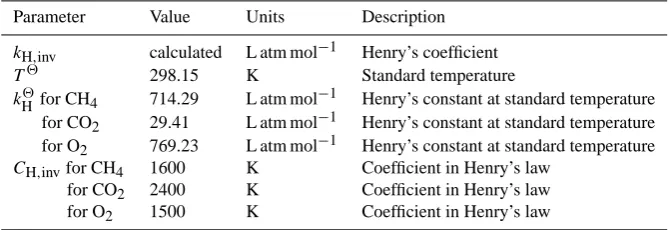
Table 2. Gas diffusion parameters taken from Sander (1999).
Parameter Value Units Description
kH,inv calculated L atm mol−1 Henry’s coefficient T2 298.15 K Standard temperature
kH2for CH4 714.29 L atm mol−1 Henry’s constant at standard temperature
for CO2 29.41 L atm mol−1 Henry’s constant at standard temperature
for O2 769.23 L atm mol−1 Henry’s constant at standard temperature
CH,invfor CH4 1600 K Coefficient in Henry’s law
for CO2 2400 K Coefficient in Henry’s law
for O2 1500 K Coefficient in Henry’s law
peatland vegetation is negligible and choose to set the wind speed in LPJ-WHyMe to a constant value ofU10=0 m s−1.
The Schmidt numbers for carbon dioxide and methane can be deduced from J¨ahne et al. (1987) by fitting a third-order polynomial to the observations, following Riera et al. (1999). The coefficients to estimate the Schmidt number for oxygen were taken from Wanninkhof (1992). The resulting relations give
ScCH4=1898−110.1T+2.834T
2−0.02791T3, R2=1;p <0.001
ScCO2=1911−113.7T+2.967T
2−0.02943T3,
R2=1;p <0.001 (7)
ScO2=1800.6−120.1T+3.7818T
2−0.047608T3,
whereT is temperature in◦C.
The concentration, Ceq, in Eq. (4), in mol L−1, of a dissolved gas in equilibrium with the gas partial pressure,
ppartial, above the solution can be estimated using Henry’s law as Ceq=ppartial/ kH,inv, where kH,inv is Henry’s
coef-ficient in units of L atm mol−1. For methane in the
atmo-sphere,ppartial=pCH4=1.7 ×10⁻⁶atm. The temperature
dependence of Henry’s coefficient is given by logkH,inv(T )=logk2H−CH,inv
1 T −
1
T2
, (8)
whereT is temperature in K,k2H is Henry’s constant at stan-dard temperature T2, and CH,inv is a coefficient (Sander,
1999). Table 2 lists values and units for these parameters. In the case of methane and carbon dioxide, the surface concentration Csurf will be greater than Ceq andJ will be negative, indicating flux from the soil to the atmosphere. For oxygen, the balance will be reversed andJ will be positive, indicating flux of gas into the soil.
2.5.1 Diffusivity of gases
The molecular diffusivitiesDCH4,DCO2 andDO2 depend on
temperature, the amounts of water and air in the soil and the soil porosity. We derive diffusivities in water by fitting a
quadratic curve to observed diffusivities at different temper-atures (Broecker and Peng, 1974), giving
DCH4,water=0.9798+0.02986T+0.0004381T2, R2=1;p <0.001,
DCO2,water=0.939+0.02671T+0.0004095T2,
R2=0.97;p <0.001, (9)
DO2,water=1.172+0.03443T+0.0005048T2, R2=1;p <0.001
whereT is the soil temperature in◦C andD•,wateris the
dif-fusivity of methane, carbon dioxide and oxygen in water in 10−9m2s−1.
For diffusion in air, we use values given by Lerman (1979) to find the dependence of diffusivities on the temperature:
DCH4,air=0.1875+0.0013T ,
DCO2,air=0.1325+0.0009T , (10) DO2,air=0.1759+0.00117T ,
whereT is the soil temperature in◦C and D•,air is the
dif-fusivity of methane, carbon dioxide and oxygen in air in 10−4m2s−1.
For diffusion through soil, we also need to take account of the effect of soil porosity on the diffusivity. Our esti-mation of the diffusivity in porous soil,D•,soil, follows the
Millington-Quirk model (Millington and Quirk, 1961). It has been shown by Iiyama and Hasegawa (2005) that this model gives better results for peat soils than the Three-Porosity-Model (Moldrup et al., 2004), which has only been tested for mineral soils. Using the Millington-Quirk approach, we find
D•,soil=
(fair)10/3
82 D•,air, (11)
whereD•,soilis the overall diffusivity of a gas in porous soil, fair is the fraction of air (or the air-filled porosity as it is
termed by Millington and Quirk) and8is the overall poros-ity. D•,airis the diffusivity of the respective gas in air from
For layers wherefair≤0.05, the diffusivities for water are used. Whenfair>0.05, the diffusivities in air, which are four orders of magnitude larger than those in water, become more important, and the values calculated in Eq. (11) are used. The final diffusivities,D•are thus
D•=
D•,water, fair≤0.05,
D•,soil, fair>0.05. (12)
2.6 Transport through aerenchyma
The second pathway for methane and carbon dioxide to es-cape to the atmosphere and for oxygen to enter the soil is via transport through vascular plants. Some vascular plants adapt to inundation by developing aerenchyma, gas-filled tis-sue in roots, rhizomes, stems and leaves. As well as their main adaptive function of delivering oxygen to the roots, aerenchyma constitute direct conduits for the transport of methane and carbon dioxide from the soil to the atmosphere. Gases transported through aerenchyma either follow a con-centration gradient or are actively pumped upwards. Here, we consider only the passive flux of methane and carbon dioxide through plants as it is the most dominant form of gas transport (Cronk and Fennessy, 2001). The main factors for transport through aerenchyma are thus (i) the abundance of aerenchymatous plants; (ii) the biomass of aerenchymatous plants; (iii) the phenology of aerenchymatous plants, i.e. the period roots, stems and leaves are available for gas transport; and (iv) the rooting depth of aerenchymatous plants, which determines the depth to or from which gas can be transported. Forbs (herbaceous plants other than grasses) can have aerenchyma, but their contribution to the overall net primary production (NPP) in peatlands is generally small compared to graminoids (Weltzin et al., 2000; Camill et al., 2001). Dwarf shrubs, which may contribute more significantly to the net primary production than forbs, do not have aerenchyma. Therefore, forbs and dwarf shrubs were not included in LPJ-WHyMe, although we recognise that dwarf shrubs may con-tribute significantly to net primary production of peatlands and influence CH4emissions via root exudates. It is
there-fore desirable to include dwarf shrubs into future versions of our model.
Before methane enters the plant tissue a relatively large proportion is oxidised in the highly oxic zone around the roots, where methanotrophs thrive. Rhizospheric oxidation is species dependent and can reach 100% in Juncus effusus L. and Eriophorum vaginatum L., but can be much lower in e.g. Carex rostrata with 20–40% oxidation (Str¨om et al., 2005).
Plant-mediated transport in LPJ-WHyMe occurs solely via the flood-tolerant C3 graminoid plant functional type, with
the gas flux through vascular plants being related to the cross-sectional area of tillers3available to transport gas. The
3Tillers are segmented stems produced at the base of many
plants in the family Poaceae, with each stem possessing its own
mass of the tillersmtiller is estimated by multiplying the leaf biomass of graminoids (bgraminoidleaf ) by the daily phenology,ϕ:
mtiller=bgraminoidleaf ϕ. (13) The daily phenologyϕdescribes the fraction of potential leaf cover that is fully developed, e.g. deciduous plant functional types have zero leaf cover in winter and build up their leaf cover over the first few growing months. Maximum leaf cover is reached after a given number of growing degree days but can be modulated by drought stress. The tiller biomass
mtilleris divided by the average weight of an individual tiller
to obtain the number of tillers,ntiller. The average observed
tiller biomass for Eriophorum angustifolium Honckeny and Carex aquatilis Wahlenb. in Alaska was 0.48 g dry matter per tiller, which corresponds to 0.22 g C per tiller, assuming a carbon content of 45% (Schimel, 1995). The cross-sectional area of tillers,Atiller, is derived by multiplying the area of an individual tiller,π rtiller2 , wherertilleris the tiller radius, by the number of tillers,ntillerand the tiller porosity,8tiller:
Atiller=ntiller8tillerπ rtiller2 . (14)
A first estimate of the tiller radius,rtiller, was derived by av-eraging over the two widespread species Eriophorum angus-tifolium (3.95 mm) and Carex aquatilis (1.9 mm) (Schimel, 1995), yielding rtiller=2.9 mm. The tiller porosity is
ini-tially set to 50% (Cronk and Fennessy, 2001). Schimel (1995) also measured E. scheuchzeri Hoppe whose tillers contained only 0.09 g dry matter and whose tiller radius was 0.85 mm. Using these values to calculate the tiller cross-sectional area gives a similar value to that based on our val-ues above (0.48 g drymatter and 2.9 mm radius) for the same biomass. In Sect. 4.2, the sensitivity of methane emissions to the tiller radius and porosity is tested.
Finally, each layer is allocated a fraction of the total cross-sectional area of tillers according to the respective root frac-tion in that layer.
2.7 Ebullition
An upper limit on the quantity of dissolved methane is im-posed, with the maximum solubility of methane at a given temperature following Yamamoto et al. (1976). The best-fit curve through Yamamoto et al.’s observations is
SB=0.05708−0.001545T+0.00002069T2, (15)
whereSBis the Bunsen solubility coefficient, defined as vol-ume of gas dissolved per volvol-ume of liquid at atmospheric pressure and a given temperature. We use the ideal gas law to convert the volume of methane per volume of water into moles as
n=pV /RT , (16)
Table 3. Sensitivity test parameters.
CH4/CO2 CH4/CO2production ratio under
anaer-obic conditions
foxid Fraction of available oxygen used for
methane oxidation
fexu Fraction of NPP put into exudates pool k10exu Turnover rate for exudates pool
Rmoist Moisture response, used to weight de-composition rates for exudates, litter, fast and slow carbon pools
8tiller Tiller porosity rtiller Tiller radius
wherep=patm+ρgzis the sum of the atmospheric and hy-drostatic pressures (Pa), calculated from the density of water (ρ), acceleration due to gravity (g) and water height (z),V is the methane volume (m3),T is the temperature (K), the gas constantR is 8.3145 m3Pa K−1mol−1 andnis the amount
of gas (mol). Atmospheric pressure has been shown to be a trigger for ebullition (Tokida et al., 2007), but atmospheric pressure is not yet used as an input variable for LPJ-WHyMe and is therefore assigned a constant value. Any methane in excess of the maximum solubility is immediately released to the atmosphere in form of ebullition.
3 Evaluation sites and experimental setup 3.1 Method for sensitivity test
We performed an initial sensitivity experiment for seven pa-rameters, for which there were little or no data available and for which the choice of parameter values was therefore the most uncertain. The parameters used are listed in Table 3 and the values used in each sensitivity experiment are shown in Table 4.
The sensitivity results were summarised by regressing the different methane fluxes, i.e. plant-mediated, diffusion, ebul-lition, and total flux, against each set of parameter values. Fluxes were normalised by the maximum of each flux type for each site to enable comparison of regression slopes be-tween sites and flux types.
3.2 Method for parameter fitting
After the initial sensitivity test, we conducted a parameter fitting exercise. For the parameter fitting, we used only three values per parameter (see right hand side of Table 4), but this time, we ran the model for all of the possible 2187 different combinations in the parameter space. The monthly modelled
values were compared to monthly observed values and the root mean square error (RMSE) was calculated
RMSE(m,o)=
s Pn
i=1(mi−oi)2
n , (17)
wheremare the modelled ando the observed values; nis the number of months for which we had observed values. In order to compare the statistics between sites, we normalised the RMSE (NRMSE) by the standard deviation of the obser-vations SDo.
NRMSE=RMSE/SDo. (18)
We used the lowest average NRMSE over all seven sites to find the best overall parameter combination and the lowest individual NRMSE to find the best site-specific parameter combination.
3.3 Input data for LPJ-WHyMe
Input data needed to drive LPJ-WHyMe are climate data and atmospheric CO2concentrations. Soil texture information is
not required as all grid cells for which LPJ-WHyMe is run are set to the organic soil type. For the site-by-site compari-son we used the Climate Research Unit time series data CRU TS 2.1 (Mitchell and Jones, 2005), which provides monthly air temperature and cloud cover, monthly total precipita-tion and monthly number of wet days from 1901–2002 on a 0.5◦×0.5◦grid. The time series data were used to permit effective comparison of individual model years to observa-tions. Atmospheric carbon dioxide concentrations for 1901– 2002 were taken from Etheridge et al. (1996) and Keeling and Whorf (2005). For model spin-up, the first 10 years of the CRU data were repeated until 1000 years of spin-up time had been completed. Potential problems with this spin-up procedure for peatlands are discussed in Wania et al. (2009b). 3.4 Observations
The sites used for sensitivity study, parameter fitting and model evaluation are summarised in Table 5.
3.4.1 Site 1: Michigan, USA
Table 4. Values for parameter sensitivity test and parameter adjustment.
Sensitivity test Parameter adjustment Final Parameter Units Value 1 Value 2 Value 3 Value 4 Value 1 Value 2 Value 3 value CH4/CO2 – 0.1 0.2 0.3 0.4 0.1 0.2 0.3 0.1
foxid – 0.3 0.5 0.7 0.9 0.5 0.7 0.9 0.5
fexu – 0.05 0.10 0.15 0.20 0.05 0.10 0.15 0.15
kexu10 weeks 7 13 26 39 7 13 26 13
Rmoist – 0.2 0.3 0.4 0.5 0.2 0.3 0.4 0.4
8tiller % 60 70 80 90 70 80 90 70
rtiller mm 3 4 5 6 3 4 5 3
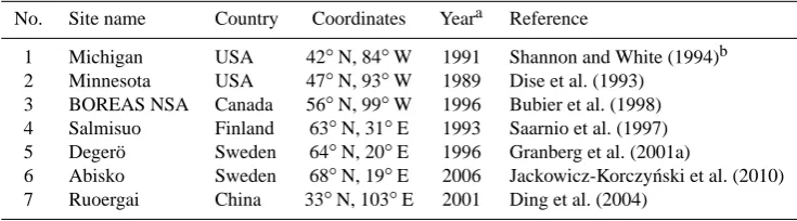
Table 5. Sites used for sensitivity analysis and methane emissions evaluation.
No. Site name Country Coordinates Yeara Reference
1 Michigan USA 42◦N, 84◦W 1991 Shannon and White (1994)b 2 Minnesota USA 47◦N, 93◦W 1989 Dise et al. (1993)
3 BOREAS NSA Canada 56◦N, 99◦W 1996 Bubier et al. (1998) 4 Salmisuo Finland 63◦N, 31◦E 1993 Saarnio et al. (1997) 5 Deger¨o Sweden 64◦N, 20◦E 1996 Granberg et al. (2001a)
6 Abisko Sweden 68◦N, 19◦E 2006 Jackowicz-Korczy´nski et al. (2010) 7 Ruoergai China 33◦N, 103◦E 2001 Ding et al. (2004)
aYear of observational data used.bData were digitised from Walter and Heimann (2000) as they plotted average values over three microsites.
at the nearby weather station in Lansing, Michigan (http: //www.nrcc.cornell.edu).
3.4.2 Site 2: Minnesota, USA
The Minnesota site is located in the US Forest Service Mar-cell Experimental Forest. Methane flux data from Junc-tion Fen are used for the model-data comparison. JuncJunc-tion Fen is a poor fen which receives some runoff from the sur-rounding uplands; lacking an outlet, it is wetter than nearby peatland sites. Vegetation is dominated by a sedge (Carex oligosperma Michaux) with some arrow-grass (Scheuchze-ria palustris) and cranberry (Vaccinium oxycoccus). The graminoids grow above a peat moss mat composed of Sphag-num angustifolium (C. Jens. ex Russ) C. Jens., S. capilli-folium (Ehrh.) Hedw. and S. fuscum (Schimp.) Klinggr. Mean annual temperature (1961–1990) is 3◦C and mean an-nual precipitation is 770 mm (Dise, 1993).
3.4.3 Site 3: BOREAS Northern Study Area, Canada The BOREAS Northern Study Site is located in central Manitoba near Thompson, and is a fen site with vegeta-tion consisting of a variety of peat mosses (Sphagnum spp.), brown moss species (Drepandocladus exannulatus (B.S.G.) Warnst.), bogbean (Menyanthes trifoliata L.) and sedges (Carex spp.) (Joiner et al., 1999). The sparse overstorey con-sists of larch (Larix laricina (Du Roi) K. Koch) and bog birch
(Betula glandulosa Michx.) (Joiner et al., 1999). Methane fluxes from several micro-sites are available for the Collapse Fen and Zoltai Fen (Bubier et al., 1998) and were used in this study. Mean January temperature is−25.0◦C and mean July temperature is 15.7◦C; mean annual precipitation is 536 mm (Gower et al., 2001).
3.4.4 Site 4: Salmisuo, Finland
The Salmisuo mire complex is situated in eastern Finland and consists of a minerogenic, oligotrophic low-sedge Sphagnum papillosum (Lindb.) pine fen (Saarnio et al., 1997). Methane fluxes from both lawn micro-sites were used for our study. The lawn habitats are vegetated by cottongrass (Eriophorum vaginatum L.), with bog-rosemary (Andromeda polifolia L.), cranberry (Vaccinium oxycoccus) and a sedge (Carex pau-ciflora Lightf.). The moss layer is dominated by S. angus-tifolium (Russow) C. Jens., S. balticum (Russow) C. Jens., with some S. magellanicum Brid. and S. papillosum Lindb. (Saarnio et al., 1997). Mean annual air temperature (1971– 2000) is 2.0◦C, with temperatures in January of−11.9◦C and in July of 15.8◦C; mean annual precipitation is 600 mm (Alm et al., 1999).
3.4.5 Site 5: Deger¨o, Sweden
from the Gulf of Bothnia (Granberg et al., 2001b). Methane data were collected in the poor fen community which is dominated by cottongrass (Eriophorum vaginatum), cran-berry (Vaccinium oxycoccus), bog-rosemary (Andromeda po-lifolia), arrow-grass (Scheuchzeria palustris), and a sedge (Carex limosa L.). The moss layer is dominated by Sphag-num balticum, S. majus (Russ.) C. Jens. and S. lindbergii Schimp. in Lindb. (Granberg et al., 2001a). Mean annual temperature (1961–1990) is 2.3◦C, with temperatures in Jan-uary of−12.4◦C and in July of 14.7◦C; mean annual precip-itation is 523 mm (Granberg et al., 2001b).
3.4.6 Site 6: Abisko, Sweden
The subarctic Stordalen mire is part of the Abisko research area in northern Sweden. Since 2006, methane fluxes have been recorded using an eddy-covariance flux tower and even though at the time of our research we did not have the model input data available for 2006, we decided to use the eddy-covariance data as they represented one of the first such data sets. These half-hourly methane data provide a high-resolution data set for this site. The flux tower covers a wet part of the palsa mire with cottongrass (Eriophorum vagina-tum) and a brown moss (Drepanocladus sp.) as dominant species. The peat is underlain by permafrost with a max-imum active layer depth of about 70–80 cm for the period 2000–2002 (Christensen et al., 2004). The mean annual air temperature (1913–2003) in Abisko, which lies 10 km west of Stordalen, is −0.7◦C with temperatures in January of
−10.9◦C and in July of 11.6◦C; mean annual precipitation is 304 mm (Johansson et al., 2006).
3.4.7 Site 7: Ruoergai, China
The Ruoergai plateau lies on the eastern edge of the Qinghai-Tibetan plateau at 3400 m altitude. The peatland area on the Qinghai-Tibetan plateau is estimated to exceed 32 000 km2, constituting 45% of China’s wetlands and 75% of China’s peatlands (Ding et al., 2004). Methane emissions from the Qinghai-Tibetan plateau peatlands are estimated to be around 0.45 Tg CH4a−1 (Ding et al., 2004). The peatland on the
Ruoergai Plateau is dominated by two sedges, Carex mey-eriana Kunth. and C. muliensis and we used the observa-tions from these two vegetation types in our analyses. Mean annual temperature is 1◦C with a minimum temperature of
−10.7◦C in January and maximum temperature of 10.3◦C in July; mean annual precipitation is 650 mm (Ding et al., 2004).
This site is included in our study as a representative of high altitude peatlands, for comparison with the behaviour of high latitude peatlands. Although our focus here is on the high latitudes, we can thus provide an initial evaluation of the suitability of LPJ-WHyMe for the simulation of methane fluxes from high altitude environments at low latitudes.
Note: The CRU mean annual temperature for the grid cell corresponding to the Ruoergai study site, with coordinates 32◦470N, 102◦320E, deviated from the observed climate by +3◦C. We suspect that this is due to the steep topography in this region, where a small error in location may lead to a large change in climate. To compensate for this effect, we therefore use the adjacent grid cell to the west, which has a mean annual temperature of 1.4◦C (minimum −10.5◦C, maximum 11.4◦C, for the period 1998–2002). These values are similar to the observed climate and are expected to pro-vide a better fit of model results to observed methane fluxes.
4 Results
4.1 Vegetation and land surface processes
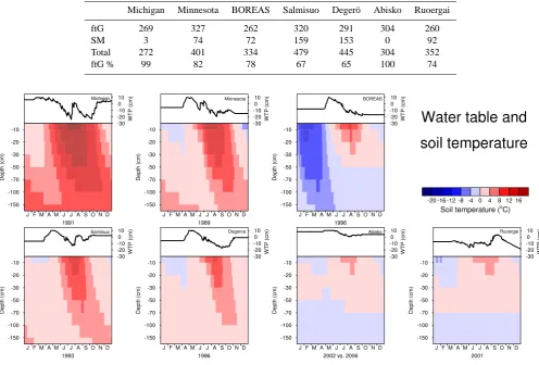
Net primary production, soil temperature and water table po-sition simulated by LPJ-WHyMe (Fig. 3) are presented to provide a framework for the interpretation of methane emis-sion results. Wania et al. (2009a) deals with the evaluation of the simulation of soil temperature and water table position in LPJ-WHyMe in detail – we present these results here to provide context for the ensuing discussion of methane flux results. The purpose of the development of LPJ-WHyMe is to create a model that is applicable on a circumpolar scale without the need for additional input data, such as vegetation composition or biomass estimates that are usually not avail-able for remote areas. Therefore vegetation composition was allowed to evolve freely. Total net primary production for the seven test sites ranges from 272 to 479 gC m−2a−1(Table 6),
which includes both aboveground and belowground net mary production. The percentage of Sphagnum moss net pri-mary production ranges from 0–35% of total net pripri-mary pro-duction, which means that flood-tolerant C3graminoids are
the dominant PFT in terms of net primary production. A dis-cussion of LPJ-WHyMe’s simulated net primary production values can be found in Wania et al. (2009b).
Permafrost occurs at the BOREAS, Abisko and Ruoergai sites, diagnosed by soil temperatures in deeper soil layers that never rise above 0◦C (Fig. 3). Since the BOREAS and Abisko sites lie in the zone of discontinuous permafrost, it is not unrealistic for LPJ-WHyMe to simulate permafrost con-ditions.
Table 6. Simulated net primary production (NPP), including above- and belowground production, for the seven test sites. Net primary
production is shown for the flood-tolerant C3graminoid PFT (ftG), Sphagnum moss PFT (SM) and totalled over all plant functional types
(all values in g C m−2a−1). Note that the total net primary production equals the sum of the C3graminoid PFT and Sphagnum PFT as
no other plant functional types contributed to the net primary production at these sites. The fraction of net primary production due to flood-tolerant C3graminoids (ftG %) is also shown.
Michigan Minnesota BOREAS Salmisuo Deger¨o Abisko Ruoergai ftG 269 327 262 320 291 304 260
SM 3 74 72 159 153 0 92
Total 272 401 334 479 445 304 352 ftG % 99 82 78 67 65 100 74
Fig. 3. Simulated water table position (line graphs) and soil temperature (contours) at the seven test sites.
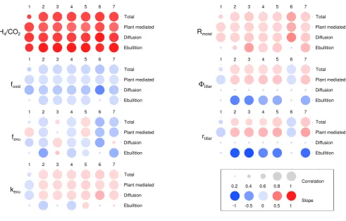
4.2 Sensitivity test
The impact of seven parameters on total methane flux as well as plant-mediated transport, diffusive flux and ebullition was tested by using four levels for each parameter. Results are summarised in Fig. 4. The parameters CH4/CO2,foxid, fexu,kexu10 andRmoist influence the production or oxidation
of methane, while8tiller andrtiller affect methane transport
pathways. Values used for each parameter are listed in Ta-ble 4.
4.2.1 Methane/carbon dioxide ratio, CH4/CO2
The results in Fig. 4 show that the most important parame-ter – indicated by the darkest colours – for all fluxes is the ratio of methane to carbon dioxide production under anaer-obic conditions, CH4/CO2. As expected, higher CH4/CO2
leads to greater methane emissions as more of the carbon is channeled into the CH4 pool. Plant-mediated transport
in-creases marginally less (lighter red colour) than the other fluxes, most likely because the capacity for plant-mediated transport is limited by the availability of tillers and can sat-urate, so that additional methane escapes via ebullition and diffusion.
4.2.2 Oxidation fraction,foxid
The greater the fraction of available oxygen used for the oxidation of methane, foxid, the less methane is emitted.
Fig. 4. Schematic summary of the sensitivity test. Numeric labels correspond to the site numbers in Table 5 and an explanation of the
acronyms for the parameters can be found in Table 3. Correlations between parameter variations and changes in methane fluxes are expressed by coloured circles of different sizes. The size of the circle represents the correlation coefficientr2, with bigger circles showing higherr2
values. The colours represent the regression slope, with darker colours indicating steeper slopes and hence a strong increase (red) or decrease (blue) in methane fluxes with increasing parameter value (slope values were capped at−1 and 1). The parameters8tillerand rtillerinfluence
the transport pathways and all others affect production or oxidation of methane.
leads to decreased methane concentrations and affects plant-mediated transport and ebullition.
4.2.3 Fraction of exudates,fexu
The fraction of exudates has a small effect in both directions. Both increases and decreases in methane fluxes are seen at sites 1, 5 and 7, while sites 2, 3, 4 and 6 show slopes in only one direction with increasingfexu (note that we count
the small blue dot for site 3 and plant-mediated transport as having a low correlation value and no notable slope). The effect of increasingfexuis complex: higherfexuvalues lead to more exudates being available for methane production, but
fexuis subtracted from the net primary production, which can lead to an overall negative effect on methane emissions due to a reduction in leaf biomass, which is used to calculate tiller biomass (Eq. 13).
4.2.4 Exudate turnover rate,k10
exu
Changes in the decomposition rate of exudates,k10exu, affected site 1 in a negative way and the other sites in a mainly posi-tive way. Ebullition was the flux least affected by changes in
k10exu, most likely because ebullition was low to start with. 4.2.5 Moisture response,Rmoist
The moisture response,Rmoist, used to calculate decomposi-tion rates, had a positive effect on almost all methane fluxes: only ebullition for two sites remained the same (small light blue dots). HigherRmoist values led to faster turnover times (Eq. 1), which increased the availability of carbon and en-hanced CH4emissions slightly.
4.2.6 Tiller porosity,8tiller
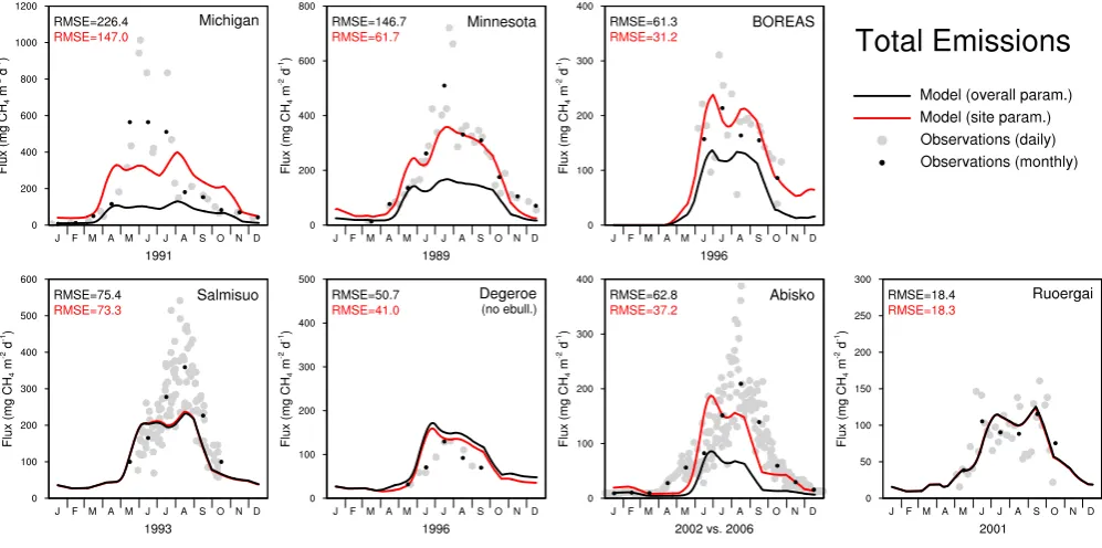
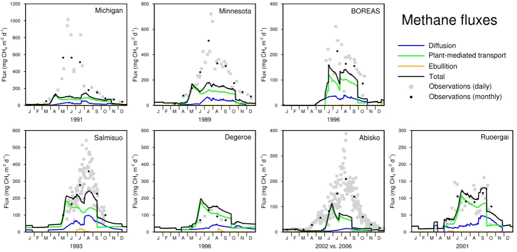
Fig. 5. Modelled methane emissions compared to observations for seven sites. Model results are plotted as 30-day running mean for the
best overall parameter combination (black line) and for the best site-specific parameter combination (red line); the respective RMSE values (mg CH4m−2d−1) are given in the top left corner of each box and follow the same colour code. Observations are plotted as daily values
(grey dots) and as monthly averages of daily values (black dots). Note that the scale of y-axes varies between plots.
the escape pathway for methane via plant-mediated transport, but at the same time it enhances the oxygen transport into the soil. At five sites, higher8tiller values increase the
plant-mediated flux while at the same time decreasing the ebulli-tion flux. The overall effect is positive for four out of the five sites as shown by the total fluxes. Diffusion is not affected by this nor the next parameter.
4.2.7 Tiller radius,rtiller
The tiller radius is used in the same equation as the tiller porosity, i.e. Eq. (14). A larger tiller radius has a simi-lar effect on plant-mediated transport to tiller porosity as it increases gas diffusion through plants. The sensitivity test shows that the range of parameter values chosen for the tiller radius (see Table 4) influences the balance between plant-mediated transport and ebullition slightly more than the tiller porosity. Plant-mediated transport shows a somewhat stronger increase and ebullition a stronger decrease when tiller radius is varied than when the tiller porosity is varied. The effect on the total methane flux is weaker as indicated by the lower correlation for sites 2–4 but is similar to the impact of varying tiller porosity.
4.3 Parameter fitting
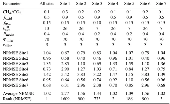
Modelled and observed methane emissions for seven sites are shown in Fig. 5. As the main purpose of the development of
LPJ-WHyMe is to simulate circumpolar methane emissions it is necessary to choose a single set of model parameters that can be applied to all grid cells. We used the parameter fitting exercise to determine which parameter set leads to the small-est overall error expressed as RMSE (black lines in Fig. 5), but we also wanted to show how much better the model can perform when tuned to individual sites (red lines in Fig. 5). The results shown in Fig. 5 are based on the parameter values and the statistics listed in Table 7. Figure 6 and Table 8 give details about the contribution of individual fluxes given the best overall parameter combination.
4.3.1 Michigan
LPJ-WHyMe cannot replicate the observed methane fluxes at the Michigan study site. The RMSE is, at 226.4 mg CH4m−2d−1, the largest of all the sites. Using
the site-specific parameter values increases the methane flux, causing a reduction in the RMSE to 147.0 mg CH4m−2d−1,
which is still the highest value of all seven sites. The increase in methane flux from the best-overall parameter values to the site-specific ones is achieved by increasing the parameters CH4/CO2,foxid andk10exu (Table 7) indicating an
underesti-mation of methane production when using the overall best parameter combination.
Table 7. Parameter fitting summary. The entries in the top half of the table indicate parameter values that lead to the lowest average NRMSE
over all sites and the parameter values used to achieve the lowest NRMSE for each particular site. The lower half of the table gives the NRMSE values for each site given the parameter combination above. The 2187 (37) combinations used for each site were ranked based on the best average NRMSE over all sites and this rank is listed in the bottom row. The rank can be used as an indication of how close the fit of the best overall parameter set is compared to the fit of the site-specific parameter set.
Parameter All sites Site 1 Site 2 Site 3 Site 4 Site 5 Site 6 Site 7 CH4/CO2 0.1 0.3 0.2 0.2 0.1 0.1 0.2 0.1
foxid 0.5 0.9 0.5 0.9 0.5 0.9 0.5 0.5
fexu 0.15 0.15 0.15 0.10 0.15 0.15 0.15 0.15
k10exu 13 26 26 7 26 7 26 7
Rmoist 0.4 0.4 0.4 0.2 0.4 0.2 0.4 0.4
8tiller 70 70 70 70 70 70 70 70
rtiller 3 3 3 3 3 3 3 3
NRMSE Site1 1.04 0.67 0.79 0.83 1.04 1.07 0.79 1.04 NRMSE Site2 0.96 0.58 0.40 0.46 0.96 1.01 0.40 0.96 NRMSE Site3 1.35 2.85 1.10 0.69 1.33 1.59 1.10 1.36 NRMSE Site4 0.73 2.90 1.27 1.03 0.71 0.84 1.27 0.75 NRMSE Site5 1.42 5.42 3.83 3.22 1.47 1.15 3.83 1.39 NRMSE Site6 0.95 0.64 0.56 0.74 0.92 1.10 0.56 0.96 NRMSE Site7 0.68 6.31 2.96 2.38 0.70 0.85 2.96 0.68 Average NRMSE 1.02 2.77 1.56 1.34 1.02 1.09 1.56 1.02 Rank (NRMSE) 1 1609 900 733 2 186 900 3
Table 8. Simulated plant mediated transport, diffusion, ebullition and total CH4fluxes (g CH4m−2a−1) from seven test sites using the
overall best parameter set. Percentage values in parentheses list the contribution of each flux type to the total flux.
No. Site Name Plant Diffusion Ebullition Total 1 Michigan 16.93 (75.6%) 5.45 (24.4%) 0.00 (0.0%) 22.38 2 Minnesota 21.88 (76.7%) 6.53 (22.9%) 0.11 (0.4%) 28.54 3 BOREAS 11.49 (69.9%) 4.80 (29.2%) 0.14 (0.9%) 16.43 4 Salmisuo 24.51 (67.8%) 11.17 (30.9%) 0.49 (1.4%) 36.16 5 Deger¨o 19.58 (74.3%) 6.76 (25.7%) 0.22 (0.8%) 26.35 6 Abisko 7.52 (84.5%) 1.38 (15.5%) 0.00 (0.0%) 8.90 7 Ruoergai 13.22 (70.8%) 5.38 (28.8%) 0.06 (0.3%) 18.66
is about 250 mg CH4m−2d−1 (Shannon et al., 1996),
which is twice the value simulated by LPJ-WHyMe (126.2 mg CH4m−2d−1). Shannon et al. (1996) estimated
the contribution of S. palustris to total methane emissions to be between 64 and 90% and LPJ-WHyMe simulates 75.6% plant-mediated emissions (Table 8). Modelled an-nual methane flux is 22.38 g CH4m−2a−1 which is in the
range of the observations for the Big Cassandra Bog (0.2 to 47.3 g CH4m−2a−1) but lower than for Buck Hollow Bog
(66.9 to 76.3 g CH4m−2a−1) (Shannon and White, 1994).
Ebullition at this site is zero, as is the case for the Abisko site, due to the vegetation cover. The Michigan and the Abisko sites are the ones for which LPJ-WHyMe models almost ex-clusively flood-tolerant graminoids as vegetation cover (Ta-ble 6). This means that in proportion to the net primary pro-duction, there is more potential for plant-mediated transport
than at other sites and therefore less CH4is available for
ebul-lition.
4.3.2 Minnesota
The Minnesota site shows good agreement between observa-tions and simulated methane fluxes in all months but July for the site-specific parameter set (Fig. 5). The RMSE error for the site-specific combination is 61.7 mg CH4m−2d−1, but
it is more than twice as high for the overall best parameter combination. The methane fluxes are lower for the overall best parameter set and total 28.54 g CH4m−2a−1(Table 8),
which is slightly less than half of the maximum observed estimate for this site of 65.7 g CH4m−2a−1 (Dise, 1993),
Table 9. Modelled total CH4fluxes (g CH4m−2) from seven test sites for the same time period as the observations taken from the references
listed in Table 5 using the overall best parameter set.
No. Site Name Modelled Observed Notes on observations 1 Michigan 22.38 0.2–47.3 Big Cassandra Bog, 1991
66.9–76.3 Buck Hollow Bog, 1991
2 Minnesota 28.06 31.5 mean over four micro habitats, April 1989–April 1990 3 BOREAS 14.5 23.2 4 mean over two fens, June – 21 October 1996 4 Salmisuo 24.65 9.6–40 1 June – 17 October 1993
5 Deger¨o 18.66 16, 13, 18 Ebullition excluded, May–September 1995, 1996, 1997 6 Abisko 8.90 24.5 and 29.5 Gap-filled eddy-covariance data, 2006 and 2007 7 Ruoergai 14.20 8.2–15.3 165 days between May and October 2001
and ebullition is very similar to the Michigan site (Table 8 and Fig. 6).
4.3.3 BOREAS
The site-specific parameter combination deviates from the overall best parameter set in five of the seven varied param-eters (Table 7) and achieves an RMSE that is half of that of the overall best parameter combination (Fig. 5). We only had five months of observations available for this site, which should be kept in mind when comparing the site-specific and the overall best parameter sets. The site-specific parameter set continues to show relatively high methane emissions into the winter months.
For the BOREAS site, plant-mediated transport was the most important flux with 69.9% of total emissions, while diffusion contributed 29.2% and ebullition the re-mainder (Table 8). Figure 6 shows that diffusion is re-sponsible for CH4 fluxes in the shoulder season, mainly
in spring before plant growth has started. Total simu-lated methane emissions for the observational season were 14.5 g CH4m−2season−1, which underestimates the
ob-served emissions 23.2 g CH4m−2season−1(Table 9).
4.3.4 Salmisuo
The Salmisuo site is one of the two sites for which the site-specific parameter set and the best overall paramter set were almost identical (Table 7) and the RMSE differ-ence between the two parameter sets was minimal (Fig. 5). Since the RMSE for the Salmisuo site was still 73– 75 mg CH4m−2d−1, we assume that further fine-tuning of
the parameters, i.e. choosing values between the ones we used, could achieve better results for the site-specific case.
Total annual simulated emissions were 36.16 g CH4m−2a−1. Observations for the period 1
June to 17 October 1993 estimate the averaged fluxes over the different microsites including lawns, flarks and hummocks to be 27.2 g CH4m−2a−1 (Saarnio et al.,
1997). The LPJ-WHyMe emissions for the same period are 24.65 g CH4m−2a−1, within the observed range (Table 9).
A recent detailed comparison of the Salmisuo observations to LPJ-WHyMe results expands this work to multiple years and discusses successes and failures of the simulations (Forbrich et al., 2010).
4.3.5 Deger¨o
Both parameter combinations show an overestimation of CH4fluxes in three out of the five available months (Fig. 5)
for the Deger¨o site. Since we knew that the measurements at this site excluded ebullition fluxes (Granberg et al., 2001a,b), we included only plant-mediated flux and diffusion in the model results in Fig. 5. Figure 6 shows that plant-mediated fluxes alone fit the observations better than the total flux. Total annual CH4 flux is 26.35 g CH4m−2a−1 of which
74.3% is emitted via plants (Table 8). Another modelling study showed a contribution of plant-mediated transport of 52–94% (Granberg et al., 2001a). The observed range of methane emissions for May to September for the years 1995– 1997 is 16, 13 and 18 g CH4m−2, respectively (Granberg
et al., 2001a). The simulated annual plant-mediated and dif-fusive flux in our study is 26.35 g CH4m−2a−1in 1996 and
18.66 g CH4m−2for May to September 1996 (Table 9).
4.3.6 Abisko
The Stordalen mire in the Abisko region is the only site for which we used data from an eddy-covariance flux tower. The site-specific parameter set achieved good results, but the overall best parameter set increased the RMSE from 37.2 to 62.8 mg CH4m−2d−1 (Fig. 5). Even with the site-specific
parameter set, there is a timing problem with the CH4
emis-sions. The observed CH4 flux starts in April, whereas the
simulated flux switches on only in late May. The modelled fluxes also decrease too early in the season. The late start of the emissions points towards a potential problem in the mod-elled soil thermal regime as Fig. 3 shows that the top soil layer is still between −4 and 0◦C in May, when observed CH4emissions have been going for two months already.
The rather abrupt decrease of CH4emissions in August is
Fig. 6. Modelled daily methane fluxes separated by transport pathway for seven sites using the overall best parameter set. Observations
plotted as daily values (grey dots) and as monthly averages of daily values (black dots) are added for guidance.
temperature drops below the growing degree day minimum of 5◦C, leaves of deciduous PFTs are shed. The air temper-atures used to drive LPJ-WHyMe are realistic and the tim-ing of the simulated leaf sheddtim-ing in August corresponds to the observed leaf senescence in 2006 and 2007 (Jackowicz-Korczy´nski et al., 2010). However, for CH4modelling, this
sudden leaf shedding means that plant-mediated transport is cut off. In the real world methane can escape through plants even after the above ground parts have died back as tillers can still be a conduit for CH4transport (Cronk and Fennessy,
2001) at least for a while after leaf senescence. This does not happen in the model so far and it may be necessary to include this process into a future version of LPJ-WHyMe.
Plant-mediated transport contributed 84.5% to total methane emissions and diffusion made up the rest (Table 8 and Fig. 6). Total annual simulated CH4 emissions were
8.9 g CH4m−2a−1(Table 9), which is just over a third of the
observed 24.5 g CH4m−2a−1(Jackowicz-Korczy´nski et al.,
2010).
4.3.7 Ruoergai
LPJ-WHyMe achieves the best results for the Ruoergai site, with RMSE values that are almost identical for both pa-rameter combinations (Fig. 5). The availability of vege-tation biomass data made a comparison between observed and modelled biomass possible for this site. LPJ-WHyMe models net primary production of 260 g C m−2a−1(Table 6), which equates to 578 g m−2a−1dry mass (45% carbon
con-tent), in the middle of the observed net primary production range of 285–750 g m−2a−1dry mass.
The seasonality of CH4 emissions is captured
exception-ally well for this site, with a perfect interplay between the plant-mediated transport and diffusion process (Fig. 6). Ebullition is negligible and plant-mediated transport is re-sponsible for 70.8% and diffusion for 28.8% of total emis-sions.
Ding et al. (2004) estimated mean methane fluxes for the two different Carex species at the Ruoergai site to be 2.06 and 3.88 mg CH4m−2h−1 and the average growing season
length to be 165 days. This results in observed fluxes of 8.2 and 15.3 g CH4m−2per growing season, which fits the
mod-elled results of 14.20 g CH4m−2a−1for the same period well
(Table 9).
5 Discussion
LPJ-WHyMe has been designed for large-scale simulation of CH4 emissions from northern peatlands. The only
grid-cell specific inputs are climate data, CO2concentration (one
underestimates emissions, and predicts an incorrect timing of emissions. In principle the mismatch might be due to our use of data from 2002 (the last year covered by CRU TS 2.1) to compare with flux measurements from 2006. However, data from CRU TS 3.0 (T. D. Mitchell, personal communication, 2010) extending through 2006 have recently become avail-able. We have compared the 2002 and 2006 data and find little difference. Minimum, maximum and average temper-atures for the Abisko grid cell were−15.6 vs.−14.1, 10.7 vs. 10.0, and−2.9 vs.−3.0◦C, and total precipitation 603 vs. 564 mm, for 2002 and 2006, respectively. The problem is more likely due to topographic heterogeneity not represented on the grid. Climate data for 2006 as directly measured at Stordalen are−0.2◦C average temperature and 347 mm pre-cipitation, i.e. the site is warmer and drier than the grid cell as represented in CRU. Too high winter precipitation leads to a thick snow cover that unrealistically delays soil thawing in spring (Fig. 5). In addition, ground water for the nearby lake flows through the mire at about 0.6 m depth and con-tributes energy to accelerate spring thawing (T. Christensen, personal communication, 2007), a feature which the model cannot represent. Finally, the low temperature bias delays spring warming. The combination of these site-specific bi-ases leads to a strong delay and an underestimate of decom-position and methane production and emission in the model. A separate topic related in part to the climate data is the model’s inability to represent peak emission rates at five out of the seven sites (Fig. 5). The use of monthly rather than daily data is likely to be one cause. The way ebullition is modelled may also contribute. Ebullition is a complex pro-cess that depends on changes in atmospheric and hydrostatic pressure and the volumetric content of various gases (Tokida et al., 2007), which in turn depends on methane concentra-tion and the density of nucleaconcentra-tion sites for bubble forma-tion (Vesala, 2010). This last factor is especially difficult to model. We opted for a simpler representation of ebullition compared to Wania et al. (2010) but in doing so we may have limited the model’s ability to reproduce peak emissions.
Sensitivity analysis showed that the parameters most in-fluencing CH4emissions in the model are the ratio of CH4
to CO2production, and the fraction of O2 used by
methan-otrophs. The ratio of CH4 to CO2 production has a linear
effect on CH4emission. A new experimental study has
pro-vided a range of 0.03 to 0.52 from six acrotelm cores from two UK peatlands under three temperature regimes (Gallego-Sala, 2008). The fraction of oxygen used by methanotrophs,
foxid, also has a linear effect on CH4 emission. If more
O2 is used to oxidise CH4, CH4 emission will be reduced
while CO2 emission will be increased. A possible way to
improve knowledge offoxid would be to evaluate CO2 and
CH4 emissions together while balancing the stoichiometry
of CO2, CH4and O2.
The parameter fitting exercise was used to find values that gave either the best site-specific results, or the best overall results, in comparison with observations. We adopted both
approaches in order to highlight two points. One is to show how well the model can perform when tuned to local site conditions. The other is to illustrate the magnitude of error that results from the use of generic parameter values. The resulting increase in RMSE was slight at three of the sites, but much larger at the other sites: from 54% (Michigan) to 137% (Minnesota). The possible reasons for these discrep-ancies are beyond the scope of our analysis, but may relate to factors not considered in our modeling approach including (a) microtopography and (b) the biogeochemical distinction between bogs and fens, as discussed in Sect. 4.6 of Wania et al. (2009a).
6 Conclusions
This work represents the first attempt to fully couple a CH4
emission model into a DGVM framework suitable for large-scale application. The use of generic climate data and param-eter values allows large-scale simulation while unavoidably introducing some additional error compared to simulations driven by site-specific observations and/or using parameter values optimised for specific sites. The model could be run, for example, for countries to estimate peatland contributions to national greenhouse gas balance, or in palaeoclimate mode to explore causes of past variations in atmospheric CH4, or
in future scenarios (Wania, 2007) to assess potential climate feedbacks involving CH4.
Supplementary material related to this article is available online at:
http://www.geosci-model-dev.net/3/565/2010/ gmd-3-565-2010-supplement.zip.
Acknowledgements. The authors would like to thank Nathalie de Noblet-Ducoudr´e, Andy Ridgwell, Angela Gallego-Sala, Ed Hornibrook and Paul Miller for discussion of the model setup and the manuscript. The comments and suggestions by two anonymous reviewers, the editor and Timo Vesala have greatly improved this manuscript. We would also like to ac-knowledge Cynthia A. Brewer for the provision of Colorbrewer (http://www.colorbrewer2.org). RW was sponsored by a stu-dentship of the Department of Earth Sciences, University of Bristol, by the EU-Project HYMN (GOCE-037048) and by an NSERC Accelerator grant (34940-27346). IR was supported by a NERC e-Science studentship (NER/S/G/2005/13913).
Edited by: A. Ridgwell
References