www.geosci-model-dev.net/3/123/2010/
© Author(s) 2010. This work is distributed under the Creative Commons Attribution 3.0 License.
Geoscientific
Model Development
Bergen Earth system model (BCM-C): model description and
regional climate-carbon cycle feedbacks assessment
J. F. Tjiputra1,2, K. Assmann1,2, M. Bentsen2,3, I. Bethke2,3, O. H. Otter˚a2,3, C. Sturm4, and C. Heinze1,2
1University of Bergen, Department of Geophysics, All´egaten 70, 5007 Bergen, Norway 2Bjerknes Centre for Climate Research, All´egaten 55, 5007, Bergen, Norway
3Nansen Environmental and Remote Sensing Center, Thormølensgate 47, 5006 Bergen, Norway 4Bert Bolin Centre for Climate Research, Svante Arrhenius v¨ag 8 C, 106 91 Stockholm, Sweden
Received: 12 May 2009 – Published in Geosci. Model Dev. Discuss.: 8 July 2009
Revised: 8 December 2009 – Accepted: 15 December 2009 – Published: 12 February 2010
Abstract. We developed a complex Earth system model by coupling terrestrial and oceanic carbon cycle components into the Bergen Climate Model. For this study, we have gene-rated two model simulations (one with climate change inclu-sions and the other without) to study the large scale climate and carbon cycle variability as well as its feedback for the period 1850–2100. The simulations are performed based on historical and future IPCC CO2emission scenarios.
Glob-ally, a pronounced positive climate-carbon cycle feedback is simulated by the terrestrial carbon cycle model, but smaller signals are shown by the oceanic counterpart. Over land, the regional climate-carbon cycle feedback is highlighted by increased soil respiration, which exceeds the enhanced pro-duction due to the atmospheric CO2 fertilization effect, in
the equatorial and northern hemisphere mid-latitude regions. For the ocean, our analysis indicates that there are substan-tial temporal and spasubstan-tial variations in climate impact on the air-sea CO2 fluxes. This implies feedback mechanisms act
inhomogeneously in different ocean regions. In the North Atlantic subpolar gyre, the simulated future cooling of SST improves the CO2gas solubility in seawater and, hence,
re-duces the strength of positive climate carbon cycle feedback in this region. In most ocean regions, the changes in the Rev-elle factor is dominated by changes in surfacepCO2, and not
by the warming of SST. Therefore, the solubility-associated positive feedback is more prominent than the buffer capac-ity feedback. In our climate change simulation, the retreat of Southern Ocean sea ice due to melting allows an additional
∼20 Pg C uptake as compared to the simulation without cli-mate change.
Correspondence to: J. F. Tjiputra (jerry.tjiputra@bjerknes.uib.no)
1 Introduction
Understanding the interactions between climate and the global carbon cycle is crucial to accurately project future cli-mate change. Unfortunately, empirical evidence for global climate-carbon cycle interactions, as well as their feedbacks for time scales relevant to the current climate change (i.e., decadal to centennial time scales), is very limited. There-fore, such an assessment has to be attempted by applying comprehensive, fully interactive global climate-carbon cycle models (Heimann and Reichstein, 2008). Recently, state-of-the-art coupled climate-carbon cycle models have been used as key elements in understanding present and future climate change. They include sophisticated interactions between the atmosphere, ocean circulation and marine biogeochemical cycles, terrestrial biosphere as well as sea-ice. Previous in-tercomparisons (Friedlingstein et al., 2006) have proven that these models, despite their notable uncertainties, are essen-tial for predicting future interactions and feedbacks between climate-carbon components in the complex Earth system.
In this study, we couple terrestrial and oceanic carbon cy-cle models to the BCM, creating the BCM-C. The model is applied to simulate climate-carbon cycle projections for the period 1850–2100. The simulations are compared with ob-servations and validated towards other Earth system model projections. Furthermore, we analyse the regional variabil-ity of mechanisms responsible for controlling the local and global climate-carbon cycle feedback.
The manuscript is organised as follows, Sect. 2 describes the different model components used in this study as well as our coupling strategy, Sect. 3 describes the configuration and settings adopted in the model simulations performed, Sect. 4 summarizes the results and analysis of the model simulations and, finally, the manuscript is closed with discussions and conclusions.
2 Model description
The BCM-C consists of global atmospheric and oceanic gen-eral circulation models coupled to oceanic and terrestrial carbon cycle models. The newly coupled model is able to interactively simulate the known global carbon-cycles pro-cesses, including the radiative feedback necessary for climate change simulations. Each component of the BCM-C is de-scribed in more detail in the following subsections.
2.1 Atmospheric circulation model
The atmosphere component is the spectral atmospheric gen-eral circulation model ARPEGE from M´et´eo-France (D´equ´e et al., 1994). The ARPEGE model, as applied in this study, is described in detail in Furevik et al. (2003) and its major features are briefly summarized here.
In ARPEGE, the representation of most model variables is spectral (i.e., scalar fields are decomposed on a truncated basis of spherical harmonic functions). In the present study, ARPEGE is run with a truncation at wave number 63 (TL63),
and a time step of 1800 s. the grid point calculations are done with a grid of horizontal resolution of about 2.8◦×2.8◦. A total of 31 levels is employed, ranging from the surface to 0.01 hPa (20 layers in the troposphere).
The physical parameterization is divided into several ex-plicit schemes, which each calculate the flux of mass, energy and/or momentum due to a specific physical process. Dif-ferent from the model description in D´equ´e et al. (1994), the version used in BCM contains a convective gravity drag pa-rameterization (Bossuet et al., 1998), a new snow scheme (Douville et al., 1995), a refined orographic gravity wave drag scheme (Lott and Miller, 1997; Lott, 1999; Catry et al., 2008) and modifications in deep convection and soil vegeta-tion schemes.
The vertical diffusion scheme is a first order eddy-viscosity scheme (Loui, 1979; Loui et al., 1982; Geleyn, 1988), which is popular in global models because of its
sim-plicity and physical clarity. In the original version of the scheme, a feedback could be activated in the case of a very cold surface. A cooling surface involved an increase in the stability which, in turn, would prevent any heating by the atmosphere. This would accelerate the cooling until reach-ing a radiative balance that could be very cold in the polar night. This phenomenon led to a significant cold bias in the global temperature in earlier versions of BCM. To avoid the phenomenon, a limitation has been added to the Richardson number: ifRi >0, thenRi← Ri
(1+Ri/Ricr)andUric=1/Ricr,
whereRicris an upper limit for positive Richardson numbers.
The standard value forUricis 0, which comes to not applying
the above limitation. In the present version of BCM, a value of 1.2 is used forUric.
In ARPEGE, there is a mass drift due to the non-conservative form of the discretized continuity equation (M. Deque, personal communication, 2009). In order to cor-rect this, the following method has been used: every 6 h the partial pressure of dry air averaged over the globe is calcu-lated. This value is then compared with the value 983.2 hPa, which is the ERA40 average value. The difference (loss or gain of mass) is then added to the surface pressure uniformly (less than 0.1 hPa per month). With this correction, total air mass can have a seasonal cycle or a long-term drift (due to variations in water vapour content), but no drift due to non-conservation. The drawback, however, is the uniform correc-tion, since the sources and sinks may be local.
2.2 Oceanic circulation model
For tracer advection and layer thickness, the current MI-COM uses incremental remapping (Dukowicz and Baum-gardner, 2000) adapted to the grid staggering of MICOM. The algorithm is computationally rather expensive compared to other second order methods, but the cost of adding addi-tional tracers is modest. In contrast to the original transport method, incremental remapping ensures monotonicity of the tracers.
The treatment of diapycnic mixing follows the standard MICOM approach of a background diffusivity dependent on the local stability and is implemented using the scheme of McDougall and Dewar (1998). To incorporate shear instabil-ity and gravinstabil-ity current mixing, a Richardson number depen-dent diffusivity has been added to the background diffusiv-ity. This has greatly improved the water mass characteristics downstream of overflow regions. Lateral turbulent mixing of momentum and tracers is parameterized by Laplacian dif-fusion, and layer interfaces are smoothed with biharmonic diffusion.
The mixed layer depth (MLD) computed in MICOM is pa-rameterized after Gaspar (1988), through a turbulent kinetic energy balance of a one-dimensional mixed layer. It belongs to the family of Kraus and Turner (1967) type mixed-layer models. The simulated MLD is consistent with separate post-processing determination of MLD based on the prognostic density or temperature criteria.
With the exception of the equatorial region, the ocean grid in our configuration is almost regular with horizontal grid spacing approximately 2.4◦×2.4◦. In order to better resolve the dynamics near the equator, the horizontal spacing in the meridional direction is gradually decreased to 0.8◦along the Equator. The model has a time step of 4800 s and a stack of 34 isopycnic layers in the vertical coordinate, with po-tential densities ranging from 1029.514 to 1037.800 kg m−3. A non-isopycnic surface mixed layer on top provides the linkage between the atmospheric forcing and the ocean in-terior.
2.3 Sea-ice dynamical model
In this study, we applied the original sea-ice model, which had been integrated into MICOM. It is a dynamic-thermodynamic sea-ice model. It shares the same horizon-tal grid resolution. The heat, salt, and water flux exchanges between the ocean and sea-ice are handled internally. The thermodynamic part of the sea-ice model is based on Drange and Simonsen (1996). The model consists of one ice and one snow layer assuming a linear temperature profile in each layer. The temperature profile is determined by the freezing temperature at the water/ice boundary, and the balance be-tween turbulent, radiative and conductive heat fluxes at the snow/air boundary. The dynamical part of the sea-ice model uses viscous-plastic rheology based in the implementation of Harder (1996).
As an alternative to the original sea-ice model, the sea-ice model GELATO (Salas-Melia, 2002) can also be used as the sea ice component in BCM-C. As opposed to the original sea-ice, GELATO is a multi-category sea-ice model (thick-ness dependent), allowing a more precise treatment of ther-modynamics. The large scale climate state and variability modes simulated by BCM using the GELATO sea-ice model are discussed in Otter˚a et al. (2009).
2.4 Ocean carbon cycle model
The BCM-C adopts the Hamburg Ocean carbon cycle (HAMOCC5.1) model, which is based on the original work by Reimer (1993) with the extensions of Maier-Reimer et al. (2005). The current version of the model in-cludes an NPZD-type (nutrient, phytoplankton, zooplank-ton and detritus) ecosystem model following Six and Maier-Reimer (1996) with multi-nutrient co-limitations (Aumont et al., 2003). The model contains over 30 biogeochemical trac-ers, which include dissolved inorganic carbon, total alkalin-ity, oxygen, nitrate, phosphate, silicate, iron, phytoplankton and zooplankton. Fixed Redfield ratios (i.e., P:N:C:1O2) are
used for production and remineralization of biogenic mat-ter. In addition to temperature and light (i.e., according to Michaelis-Menten kinetics), the phytoplankton growth rate is also co-limited by nitrate, phosphate and iron concentra-tions. The modelled bulk phytoplankton concentration is then divided into diatom and coccolithophore compartments, based on silicate concentration. Such a silicate dependent formulation yields higher diatom fraction when the prog-nostic silicate concentration is high. The remaining phyto-plankton is then assumed to be coccolithophore. In the trop-ical oligotrophic nitrate-depleted regions, the marine ecosys-tem module accounts for atmospheric nitrogen fixation as for cyanobacteria growth. The nitrogen fixation is parameterized as the relaxation of surface layer deviation of the N:P ratio of nutrients. Thus, whenever there is more phosphate than ni-trate (i.e., based on the Redfield ratio) in the surface layer, algae fix atmospheric nitrogen which in the model is imme-diately recycled to nitrate. Particulate organic carbon, pro-duced due to the ecosystem dynamics, is exported out of the euphotic zone with a constant sinking speed. Once exported, the organic matter is remineralized at depth, and the non-remineralized particles are collected by the sediment.
The inorganic carbon chemistry in the HAMOCC5.1 model is based on Maier-Reimer and Hasselmann (1987) and is updated with the OCMIP (Ocean Carbon-cycle Model Intercomparison Project) carbon chemistry protocols. The surface pCO2 in the model is
computed prognostically as a function of alkalinity, total DIC, temperature, pressure and salinity. The dissolution of calcium carbonate at depth is computed as a function of carbonate ion saturation state and a constant dissolution rate. The air-sea gas (i.e., CO2 and O2) exchange processes are
and the difference between partial pressure tracers in air and water following Wanninkhof (1992). The gas tracer solubilities are computed according to Weiss (1970) and Weiss (1974), whereas the gas transfer velocity depends on the Schmidt number and prognostic wind speed on the surface. Also note that the model has a 12-layer sediment model, which is applicable for future, long-term model studies, for example where the buffering of anthropogenic CO2 through calcium carbonate dissolution from the sea
floor becomes important. 2.5 Terrestrial carbon model
The Lund-Postdam-Jena Model (LPJ) (Sitch et al., 2003) is a large-scale terrestrial carbon cycle model, which includes dynamical vegetation. It implements terrestrial photosynthe-sis, respiration, resource competition, tissue turnover, dy-namic vegetation population with 10 plant functional types (PFTs), soil organic and litter dynamic as well as natural fire occurrence. The soil hydrology, with 2-level soil moisture, is treated by LPJ (i.e., no direct coupling to ARPEGE). For each model grid, carbon storage is allocated into four com-partments, vegetation, litter, fast and slowly overturning soil carbon pool. The current version of the model does not in-clude land use change. The LPJ has a horizontal resolution of approximately 2.5◦×2.5◦with monthly model time step. The 2.5◦ resolution corresponds to the atmospheric model, as they run on the same grid (over land).
2.6 Coupling strategy
The OASIS coupler (Terray et al., 1995), which has been de-veloped at the National Centre for Climate Modelling and Global Change (CERFACS), Toulouse, France, has been used to couple ARPEGE with MICOM. OASIS synchronizes different model components, such that the fastest running model can wait for the other until all components are inte-grated at a complete prescribed time interval (i.e., one day). It also efficiently reads, interpolates, and transfers the ex-change fields between ARPEGE and MICOM.
The HAMOCC5.1 is coupled directly into MICOM and, therefore, has identical temporal, horizontal and vertical res-olutions. This coupling allows all biogeochemical tracers within HAMOCC5.1 to be advected along MICOM’s isopy-cnic coordinates, which resemble the real structure of the water column and avoid artificial mixing and advection in the ocean interior. The caveat of such coupling includes the problem with massless layers in the outcrop regions and the introduction of bulk mixed layer on the model topmost layer. The marine biological production occurs within the euphotic zone, which is formulated to be the minimum be-tween 90-m depth and the mixed layer depth simulated by MICOM. The biogeochemical tracers are advected by the prognostic physical fields simulated by MICOM. In addition, variables such as temperature, salinity, pressure and density
used in the computation of ocean pCO2, pH and
carbon-ate ion fields are also taken from MICOM. More detail on HAMOCC-MICOM coupling, together with series of sen-sitivity carbon cycle studies are discussed in Assmann et al. (2010). In their study, Assmann et al. use the identical MICOM and the respected sea-ice model, although differ-ent atmospheric forcing could result in differdiffer-ent ice cover. They also adopt identical coupling of the model components as well as similar spatial and temporal resolution. The car-bon chemistry in their study, however, is still based on the original HAMOCC model, whereas in this study it has been adjusted to the OCMIP carbon chemistry parameterization. Supplemental Fig. 1 (see http://www.geosci-model-dev.net/ 3/123/2010/gmd-3-123-2010-supplement.pdf) illustrates the performance of the HAMOCC5.1 in simulating the observed biogeochemical tracers’ distributions when it is forced by NCEP (Assmann et al., 2010), as compared to AOGCM as shown in this study. Overall, the differences in the model-data fit are relatively small between the two model configu-rations.
The LPJ is integrated annually at the end of each model year, and forced by monthly ARPEGE output fields of tem-perature, precipitation, cloud coverage and number of rainy days per month. The number of rainy days per month is ran-domly distributed into quasi-daily values, which is normal-ized to the Climate Research Unit (CRU) monthly precipi-tation values. The coupling of CO2gas exchange occurs at
the end of every model year, where an updated atmospheric CO2concentration is computed based on the annual fluxes
between the atmosphere and the ocean or land. Thus, the atmospheric CO2concentration is only updated once a year
for the land and ocean. Currently, the albedo feedback, due to changes in the terrestrial PFT, is not implemented, but it is part of our future research plans. In all of the model simula-tions, no form of flux adjustments is applied to the model.
3 Model simulations
A set of three model simulations adopting different config-urations and forcing fields was carried out. The first is de-signed to analyse and evaluate the steady state simulated by the model, whereas the latter two are intended latter two are intended to analyse in detail the climate-carbon cycle feed-back in the model.
3.1 Experiment REF
The REF model simulation is performed for spin up. The fully coupled BCM-C is integrated for 600 years applying constant pre-industrial atmospheric CO2 concentration at
3.2 Experiment COU
For the second simulation, we initialized the BCM-C based on the final state achieved from the REF and integrated from 1850 to 2099 forced only by anthropogenic CO2emissions.
For the period 1850–1999, carbon emissions based on ob-served records of fossil fuel burning and deforestation (Mar-land et al., 2005) are used, whereas for the period 2000–2099, the IPCC SRES-A2 emission scenario (Houghton and Hack-ler, 2002) is used.
3.3 Experiment UNC
In the third simulation, we prescribed the atmospheric CO2
concentration from the COU, but the radiative effect of atmo-spheric CO2change is removed in the model (i.e., the
atmo-spheric circulation model interacts with a constant 284.7 ppm CO2 concentration). Therefore, unlike in COU, the
simu-lated carbon cycle in UNC experiences no climate change effect (e.g., warming, change in atmosphere and ocean cir-culation, etc.). Experiment UNC was designed such that its difference with experiment COU represents how future cli-mate change affect both the terrestrial and oceanic carbon uptake. This set-up is similar to that of the C4MIP study (Friedlingstein et al., 2006).
4 Results and evaluation 4.1 Pre-industrial reference run
In general, after 600 years of spin-up (REF), the BCM-C is able to reach a steady climate state, which is to a large degree consistent with observations. The performance of spatially-averaged climate parameters simulated by BCM-C in REF is compared to the observed climatology state and summa-rized using a Taylor diagram as shown in Fig. 1. The Tay-lor diagram evaluates the model performance as a function of normalized standard deviation, centered root-mean-square (RMS), and pattern correlation (Taylor, 2001). All simulated variables are normalized by the respective observed vari-able’s standard deviation, thus, a perfect model-data fit would reside in the observation point (i.e.,σ=1, RMS=0, andr=1). The model is able to reproduce the observed 2-m surface air temperature “sat” and sea surface temperature “sst” quite re-alistically in terms of spatial and actual amplitude variabili-ties, shown by the correlation and normalized standard devi-ation close to unity. The simulated surface salinity “sss” de-viates noticeably from the observation with normalized stan-dard deviation of only 0.5. This discrepancy is mainly due to the overestimated Arctic water salinity in the model com-pared to the LEVITUS climatology SSS. The simulated pre-cipitation “prc” and mean sea-level pressure “slp” variability are comparable to the observations. Biases in the precipita-tion are mainly due to a weaker precipitaprecipita-tion rate over the ocean than that observed, whereas discrepancies between the
observed and modelled mean sea-level pressure are caused by excessive high pressure over the Arctic, which resulted in weaker Icelandic and Aleutian low pressure systems. Addi-tionally, the atmospheric meridional pressure gradient in the Antarctic circumpolar region is too weak. This resulted in weak surface winds there. Similar evaluation using the Tay-lor diagram for different seasons show similar model-data fit patterns (see supplemental Fig. 2).
The marine carbon cycle in REF produces the observed main characteristics of ocean biogeochemistry, which in-clude global distributions of nutrients, DIC, alkalinity, High Nutrient-Low Chlorophyll regions, regional net primary production and air-sea CO2 fluxes. The pre-industrial
ocean tracer distribution simulated by HAMOCC5.1 is dis-cussed in Assmann et al. (2010). We also note that because of the different atmospheric forcing fields used to force the ocean physics, the ocean biogeochemical tracer distributions are slightly different, despite nearly identical carbon cycle processes (also see supplemental Fig. 1). Within the last 100 model years of the spin-up run, the ocean carbon cycle yields steady annual air-sea CO2 fluxes, net primary production, particle organic
carbon export and calcite export of 0±0.2, 39±2.0, 9.5, and 0.6 Pg C yr−1,respectively (as shown in supplemen-tal Fig. 3, see http://www.geosci-model-dev.net/3/123/2010/ gmd-3-123-2010-supplement.pdf). The model simulates well the fundamental characteristics of oceanic CO2 fluxes
patterns, with dominant outgassing in the Equatorial Pacific and uptakes in the North Atlantic, and the Southern Ocean.
The interannual land-atmosphere carbon fluxes simulated in REF have maximum variability range of±2.0 Pg C yr−1. The pre-industrial equilibrium global terrestrial vegeta-tion, soil and litter carbon content simulated by BCM-C are 735, 1380, and 145 Pg BCM-C, respectively, consis-tent with the range of other terrestrial model studies (Kucharik et al., 2000; Sitch et al., 2003) (see also supple-mental Fig. 4, http://www.geosci-model-dev.net/3/123/2010/ gmd-3-123-2010-supplement.pdf).
4.2 Model projections of global carbon cycle and climate change
0.5 1
1.5
0 0.5
0 0.75
0 1
0 1.25
0 1.5
1 0.99 0.95 0.9 0.8 0.7 0.6 0.5 0.4 0.3 0.2 0.1 0
Standard deviation
C o r re
l at i on
C o
e f
f i
c
ie
n t
R
M
S D
obs sst sss
sat prc
slp
Fig. 1. Taylor diagram for annually-averaged sea surface temperature (sst), salinity (sss), surface air temperature (sat), precipitation (prc)
and sea level pressure (slp) from the reference run (REF) as compared to climatology Levitus and NCEP reanalysis.
180oW 120oW 60oW 0o 60oE 120oE 180oW 60oS
30oS 0o 30oN 60oN
180oW 120oW 60oW 0o 60oE 120oE 180oW 60oS
30oS 0o 30oN 60oN
0 20 40 60 80
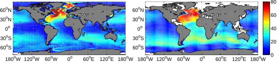
Fig. 2. Map of column integrated anthropogenic carbon content in the ocean for the year 1994 simulated by the BCM-C (left) and compared
to the observation-based estimates (right) from Sabine et al. (2004). Units are in [mol C m−2].
Globally, the time-integrated anthropogenic carbon uptake up to year 1994 is estimated to be 96 Pg C. Of this amount, the North Atlantic region account for 21%, whereas the re-gions south of –14◦S account for 47% of the global inven-tory. In general, the simulated regional anthropogenic carbon uptake is slightly stronger in the North Atlantic region along the Gulf Stream. This uncertainty may be attributed to the artificially large mixed-layer depth that allows surface car-bon to be transported into deep ocean more efficiently (Ass-mann et al., 2010). This overestimation offsets the slightly lower carbon uptake in the rest of the world ocean regions. For the same period, the terrestrial counterpart takes up ap-proximately 90 Pg C. The values above are well within error ranges given in Sabine et al. (2004).
Figure 3 also shows that the BCM-C model reproduces the observed atmospheric CO2concentrations relatively well
(i.e., 382 ppm for the present day value). In the COU sim-ulation, the atmospheric CO2 concentration is projected to
increase to 870 ppmv by 2099. This projection is well within the range given by 11 Earth system model forecasts, as shown in Fig. 3 (Friedlingstein et al., 2006).
Because the atmospheric CO2change in the UNC
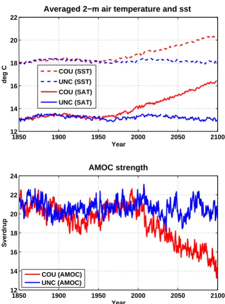
simu-lations has no radiative effect, projected temperature vari-ability remains within the pre-industrial state (see Fig. 4). In the COU simulation, the model projects an increase in global average surface atmosphere and ocean temperature by roughly 3.3◦C and 2.5◦C, respectively as shown in Fig. 4.
Atmospheric CO
2
[ppm]
1850 1900 1950 2000 2050 2100
250 450 650 850 1050
Ocean uptake [Pg C/yr]
1850 1900 1950 2000 2050 2100
−2 0 2 4 6 8 10 12
Year
Land uptake [Pg C/yr]
1850 1900 1950 2000 2050 2100
−6 −3 0 3 6 9 12 15
Fig. 3. BCM-C projection of annual (top) atmospheric CO2
con-centration, (middle) oceanic carbon uptake and (bottom) terrestrial carbon uptake as compared to the range from other models (grey shading) (Friedlingstein et al., 2006). Red lines represent results from COU whereas blue lines represent results from UNC simula-tions.
of changes in global temperature to changes in atmospheric CO2, is 0.0056◦C/ppm. This value is also within range of
0.0038–0.0082◦C/ppm obtained from the other Earth system models (Friedlingstein et al., 2006).
Changes in global temperature, in turn, alter key features of the climate system, e.g., ocean circulation, sea-ice ex-tent, precipitation, solar radiation and surface winds. These changes in fundamental climate parameters modify both the terrestrial and ocean carbon cycle, and finally feedback to atmospheric CO2concentration and the climate system. To
first order, an increase in global temperatures would reduce the average rate of carbon uptake by the terrestrial reservoir as well as the ocean.
1850 1900 1950 2000 2050 2100
12 14 16 18 20 22
Year
deg C
Averaged 2−m air temperature and sst
COU (SST)
UNC (SST)
COU (SAT) UNC (SAT)
1850 1900 1950 2000 2050 2100
12 14 16 18 20 22 24
Year
Sverdrup
AMOC strength
COU (AMOC) UNC (AMOC)
Fig. 4. Time-series of global mean (top) 2-m surface temperature
and sea surface temperature and (bottom) strength of the Atlantic Meridional Overturning Circulation as projected by the BCM-C model for both the COU and UNC simulations. There are gener-ally no significant trend changes in the UNC simulation because the changes in atmospheric CO2concentration here have no radiative
effect.
In both the COU and UNC experiments, Fig. 3 shows that the model simulates a continuous increase in atmo-spheric carbon uptake by the ocean, with annual uptake of 2.4 Pg C/yr for the present-day climate and up to 6 Pg C/yr uptake by year 2099. This increase in oceanic carbon uptake is expected as the difference between the partial pressure of CO2 in the atmosphere and ocean surface continues to
in-crease. Nevertheless, the fraction of the annual CO2
in the terrestrial carbon uptake between the COU and UNC simulation suggests that the positive global climate-carbon cycle feedback is mainly attributed to terrestrial processes. Both the simulated annual ocean and terrestrical carbon up-takes look very reasonable, located well in the middle of other model estimates also shown in Fig. 3.
The COU simulations also show a reduction in the strength of the Atlantic Meridional Overturning Circulation (AMOC) from 21 to 14 Sv by year 2099 (see Fig. 4). This change is consistent with a multi-GCMs study by Schmittner et al. (2005) and resulted in only a small reduction in the marine primary production and export production, especially in the high latitude regions. Earlier studies show that the slow down in the overturning circulation may have little oceanic carbon cycle-climate feedback for the short-period pertinent to this study. For example, Zickfeld et al. (2008) summarize that up to 2100, the increase in SST in the warmer climate, which reduces the CO2solubility is mostly responsible for the
re-duction in the carbon uptake. Note that the increase in SST also decreases the CO2buffer factor (i.e., buffer capacity
in-creases with rising T) for seawater.
For multi-century time scales, the AMOC and ocean cir-culation is generally found to be the main reason for reduced CO2uptake. For these longer time scales, the weakening of
the AMOC reduces the fluxes of upwelled nutrients to the surface, which in turn reduces the carbon uptake by the bio-logical pump.
4.3 Global climate-carbon cycle feedbacks
We applied similar formulation used in the Friedlingstein et al. (2006) study to quantify both the global ocean and ter-restrial climate-carbon feedbacks. Sensitivity of land/ocean carbon storage to changes in atmospheric CO2concentration
(βL/βO) can be computed as follows:
βO/L= 1COunc/L
1CAunc, (1)
where 1COunc/L and 1CAunc represent the change in carbon contents in the ocean/land and atmosphere, respectively, over a given simulation period in the UNC experiment. Figure 5a and c illustrate the evolution ofβO andβLsimulated by the
BCM-C as compared to the other models. In both reservoirs, there are positive and relatively linear relationships between carbon uptake and increasing atmospheric CO2
concentra-tion. For the ocean, Fig. 5a also shows that this relationship is nearly an overlap to the Max Planck Institute (MPI) mod-els, in which they apply similar ocean carbon cycle model (i.e., HAMOCC5). This implies that the global sensitivity of the HAMOCC5 component with respect to atmospheric CO2concentration is relatively robust, despite differences in
physical forcing fields. For the land, these are noticeably spread in the sensitivities between the BCM-C as compared to other models that use the LPJ as the terrestrial component.
We attribute this variation to the regionally varying physical forcing fields, particularly temperature and precipitation. In Sect. 4.4, we also discuss how the variation in regional pre-cipitation affects the regional sensitivity of carbon uptake to temperature.
Using the information from Eq. (1), we can estimate the sensitivity of ocean/land carbon uptake to change in climate (γL/O), particularly surface temperature, by solving the
fol-lowing equation:
1COcou/L=βO/L1CAcou+γO/L1Tcou, (2)
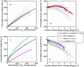
where1Tcou represents the change in global mean surface temperature simulated in the COU simulation. Figure 5b shows that the global oceanic carbon uptakes are negatively sensitive to changes in surface temperature, especially when the temperature change is greater than 2◦C. Compared to the ocean sensitivity, the terrestrial carbon storage exhibits higher sensitivity (i.e., approximately double) to temperature change (see Fig. 5d). Although there is no clear signal, the sensitivity of carbon storage to temperature changes is rela-tively comparable for models with similar carbon cycle com-ponents (i.e., HAMOCC, LPJ).
For the year 2099, the sensitivities of ocean and land car-bon storage to changes in atmospheric CO2 for the
BCM-C model is 1.0 Pg BCM-C ppm−1 and 1.5 Pg C ppm−1, respec-tively. The respective mean values for the other models are 1.1±0.25 (s.d.) and 1.4±0.58 (s.d.) for both the ocean and land sensitivities. The sensitivities of ocean and land car-bon uptake to changes in temperature are –19 Pg C K−1and – 118 Pg C K−1for the BCM-C model as compared to –30±15 (s.d.) and –79±43.7 (s.d.) for the mean from other models. 4.4 Regional terrestrial climate-carbon cycle feedbacks
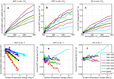
All previous coupled climate-carbon cycle models reported in the literature unanimously demonstrate a positive feed-back between terrestrial carbon cycle and climate change, mainly due to the consequences of kinetic sensitivity of pho-tosynthesis and respiration to temperature (Luo, 2007). Fi-gure 3c shows that the global terrestrial climate carbon cycle feedback simulated by our model is also positive, resulting in less uptake of approximately 323 Pg carbon when climate change is taken into account in the COU simulation. On the other hand, when climate change is excluded (i.e., in UNC simulation), the CO2fertilization effect dominates the
sim-ulated steady increase in the terrestrial carbon uptake. The feedback strength in the model is controlled primarily by the response of terrestrial photosynthesis and respiration to changes in different climate variables, such as temperature and atmospheric CO2concentration. Here, we will assess the
regional strength of the terrestrial climate carbon cycle feed-back by computing the sensitivity of regional carbon uptake, net primary production, and respiration dynamics to changes in atmospheric CO2concentration as well as surface
Cumulated ocean uptake [Pg C
]
Atmospheric CO
2 change [ppm]
a
0 200 400 600
0 200 400 600 800
Cumulated ocean uptake [Pg C
]
Surface temperature change [degree C]
b
0 1 2 3 4 5
−300 −200 −100 0 100
Cumulated land uptake [Pg C]
Atmospheric CO2 change [ppm]
c
0 200 400 600
0 250 500 750 1000
Cumulated land uptake [Pg C]
Surface temperature change [degree C]
d
0 1 2 3 4 5
−600 −400 −200 0
BCM−C (HAMOCC & LPJ)
MPI (HAMOCC)
BERN−CC (LPJ)
CLIMBER (LPJ)
Fig. 5. The sensitivity of the (a, b) oceanic carbon uptake to change in atmospheric CO2concentration and surface temperature and (c, d) terrestrial carbon uptake to change in atmospheric CO2and surface temperature. Also plotted here are similar sensitivities of the other Earth
system models (light-grey lines) and models with similar carbon cycle components: MPI (Max Planck Institute, red lines), BERN-CC (Bern Carbon-Cycle Climate model, green lines), and CLIMBER (CLIMBER2-LPJ, purple lines).
While an increase in atmospheric CO2 would generally
amplify terrestrial carbon uptake due to CO2 fertilization,
the associated climate change effect on regional terrestrial carbon cycle is less understood and predictable. The ge-ographical distribution of time-integrated terrestrial carbon uptake by year 2099 from the COU experiment is shown in Fig. 6a. By the end of the century, regions that remain prominent net carbon sinks are the equatorial regions, cen-tral and northern Asia, cencen-tral Europe, and northern Amer-ica. In the tropics, significant carbon uptake is mainly at-tributed to an increase in atmospheric CO2due to the
fertil-ization effect. At high latitudes, in addition to CO2
fertiliza-tion, an extended growing season also leads to an increase in NPP. However, in certain regions (i.e., northeastern Europe, northern and central America, and eastern Asia), where win-ter temperatures increase significantly by as much as 20◦C,
soil respiration overcomes the NPP increase, resulting in a reduced soil turnover time. In these regions, the model sim-ulates outgassing of carbon to the atmosphere by the end of the 21st century.
Figure 6b shows the difference in accumulated carbon up-take between the COU and UNC simulations. To first or-der, regions with negative values represent regions with pos-itive climate-carbon cycle feedback. Some regions, such as the equatorial Africa, Amazonia, and southeastern Australia,
take up carbon initially in the early simulation periods, but end up releasing more carbon by the end of the 21st century. The main reason for the outgassing of the tropical regions mentioned above is the reduction in NPP due to warming (see the regional sensitivity of NPP to temperature change in Fig. 7). This sensitivity is in line with study by Sitch et al. (2008). Figure 6b also shows that there are a few temperate terrestrial biosphere domains along the 30◦N and 20◦S that take up more carbon when climate change is included in the model simulations.
For the regional sensitivity of carbon uptake to atmo-spheric CO2, we applied a similar formulation as Eq. (1).
Here the sensitivity is computed for different latitudinal bands and weighted by the surface area. The latitudinal evo-lution ofβLis shown in Fig. 7a. It shows that the response
of carbon uptake due to increase in atmospheric CO2alone is
generally strongest in the equatorial regions and decreasing toward higher latitude regions. Since carbon uptake in our model is computed mainly as the difference between NPP and respiration, the sensitivities of these terms to CO2
con-centration are also computed. Generally, Fig. 7b also shows that NPP at low latitudes has the strongest CO2fertilization
Accumulated NEP COU (1850−2099)
−150 −100 −50 0 50 100 150 −60
−30 0 30 60 90
−10 −5 0 5 10
Difference [COU−UNC] (1850−2099)
−150 −100 −50 0 50 100 150 −60
−30 0 30 60 90
−10 −5 0 5 10
−6 −3 0 3 6−60 −30 0 30 60 90
[kg C/m2]
−6 −3 0 3 6−60 −30 0 30 60 90
[kg C/m2]
a
b
Fig. 6. Geographical distribution of accumulated carbon uptake by the land [Pg C] (top) simulated by the COU simulation and (bottom) the
difference between COU and UNC simulations. The right panel shows the latitudinal average of carbon uptake [kg C/m2].
assimilation rate of CO2 is more efficient in warmer
tem-peratures. Analogously, Hickler et al. (2008) show that the effect of CO2enhancement on regional plant photosynthesis
is strongest at higher temperature regions.
Interestingly, the latitudinal response of soil respiration to CO2 changes (i.e., Fig. 7c) is very similar to the response
of NPP where that higher ambient CO2concentrations lead
to higher soil respiration rates. The effect of CO2
fertiliza-tion on heterotrophic respirafertiliza-tion can be explained as follows. Higher atmospheric CO2levels reduce stomatal opening and,
hence, reduce evapotranspiration. This condition leads to the increase in water usage efficiency and increasing soil-water moisture. In addition, the increase in NPP also leads to an increase in litter input to the soil in some regions. Finally, these factors lead to an increase in soil respiration. In the low latitudes, the strong sensitivity simulated by the model is mainly due to the warm tropical temperatures and signif-icant increase in soil moisture. At high latitudes, despite an increase in litter carbon as well as soil moisture, the soil decomposition remains low in the high CO2 environment,
which may be due to the lower temperature.
In order to analyse the sensitivity of regional carbon up-take to changes in temperature alone, an additional experi-ment (UNCb) was performed by only running the LPJ model off-line. In this experiment, the LPJ is simulated for the same
period (1850–2099), forced by the climate variability from the COU simulation while maintaining constant, pre-industrial atmospheric CO2concentration. Here, the
sen-sitivity of land carbon uptake to changes in temperature can be computed as:
γL= 1CLuncb
1Tcou , (3)
where1CLuncb and1Tcou represent the change in land car-bon contents in the UNCb and change in surface tempera-ture in the COU simulations, respectively. All regions show uniform sensitivity signs, increase in carbon outgassing with higher atmospheric temperature. Figure 7d shows that tropi-cal regions have highest sensitivity towards changes in tem-perature, whereas the high latitude regions generally have lower sensitivity. In the northern hemisphere mid-latitude (30◦N–60◦N), our simulation also shows relatively large
climate-carbon cycle feedback, where future warming leads to a reduction in the annual NPP and an increase in het-erotrophic respiration. This result is in line with independent study of Cramer et al. (2001), which uses multiple dynami-cal vegetation models to assess the terrestrial climate-carbon cycle feedback.
2800 480 680 880 2
4 6 8
Atmospheric CO
2 concentration
Accumulated carbon uptake [kg C/m
2]
NEP vs atm. CO
2
a
280 480 680 880
0 0.1 0.2 0.3 0.4 0.5
Atmospheric CO
2 concentration
Annual NPP change [kg C/m
2 yr]
NPP vs atm. CO
2
b
280 480 680 880
0 0.1 0.2 0.3 0.4 0.5
Atmospheric CO
2 concentration
Annual RH change [kg C/m
2 yr]
RH vs atm. CO
2
c
0 2 4 6 8
−4 −3 −2 −1 0 1
Surface temperature change (deg C)
Accumulated carbon uptake [kg C/m
2]
NEP vs sfc. T
d
0 2 4 6
−0.08 −0.04 0 0.04 0.08
Surface temperature change (deg C)
Annual NPP change [kg C/m
2 yr]
NPP vs sfc. T
e
0 2 4 6
−0.08 −0.04 0 0.04 0.08
Surface temperature change (deg C)
Annual RH change [kg C/m
2 yr]
RH vs sfc. T
f
N90−N60
N60−N30
N30−N10
N10−S10
S10−S30
S30−S60
global
Fig. 7. Latitudinal sensitivities of (a) cumulated land carbon uptake to atmospheric CO2concentration, (b) sensitivity of annual terrestrial
NPP to changes in atmospheric CO2, and (c) sensitivity of heterotrophic respiration to changes in atmospheric CO2. Bottom figures (d, e,
and f) shows similar sensitivities to changes in surface temperature.
increase in soil respiration due to warming overtakes the in-crease in NPP due to the extended growing seasons. This mechanism would eventually lead to a significant reduction in the soil carbon turnover time by up to 25 years (not shown here) in these regions. Figure 7e and f also show that the regional sensitivity of net primary production and hetero-thropic respiration to changes in temperature is very nonlin-ear. We attribute this non-monotic sensitivity to variabili-ties of other physical forcings (i.e., precipitation) induced by changes in temperature. For example, Supplemental Fig. 5 shows that for some regions (e.g., N90-N60), the changes in temperature is relatively linear to change in precipitation. In other regions, there is no clear relationship between regional changes in temperature and precipitation.
4.5 Regional ocean climate-carbon cycle feedback
The regional oceanic carbon uptake is determined by the gra-dient between the partial pressure of CO2in the atmosphere
and surface ocean, where the latter term depends strongly on the physical state of the ocean, hence the climate variabil-ity. As a first step to analyse the regional climate-carbon cycle feedback in the ocean, we compute the carbon up-take changes with respect to the pre-industrial state, and
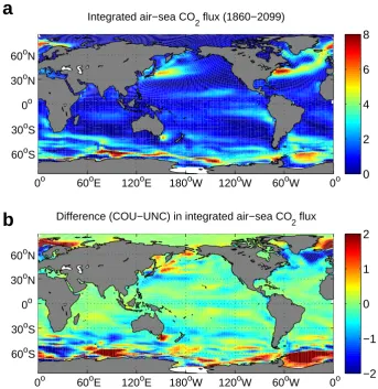
compute the difference between the COU and UNC simu-lations. Figure 8a shows a map of time-integrated changes (1860–2099) in oceanic carbon uptake relative to the ave-rage pre-industrial (i.e., 1850–1859) state. It gives estimates of regional accumulated anthropogenic carbon uptake for the experimental period. In both model runs, the model simu-lates a net anthropogenic carbon uptake in nearly all ocean regions as a result of enhanced atmospheric CO2
concen-tration. The oceanic carbon uptake through the end of the 21st century occurs mainly in the North Atlantic, northwest-ern Pacific and in the Southnorthwest-ern Ocean (South of 30◦S). In these regions, substantial carbon fluxes into the ocean cor-respond to regions with pronounced winter mixing, which is an important mechanism to transport surface DIC to a deeper ocean layer. Additionally, relative to the pre-industrial state, the COU simulation generates the largest changes in carbon fluxes in the Southern Ocean, where the anomaly of carbon uptake is as high as 10 kg C/m2over the entire model inte-gration period (see Fig. 8a).
Southern Ocean (between 30◦S and 50◦S), North Atlantic
and parts of northwestern Pacific regions. Positive values are most pronounced in the high-latitude Southern Ocean, the Arctic regions, southeast Australia and in the western bound-ary currents along the North Pacific.
4.5.1 Temporal climate change impact on regional air-sea CO2fluxes
Figure 8b also shows that the impact of climate change on regional CO2fluxes is spatially inhomogeneous. In order to
analyse the temporal impact of climate change on regional carbon uptake, we compute the difference (COU-UNC) in spatially-integrated annual carbon uptake (shown in Fig. 9).
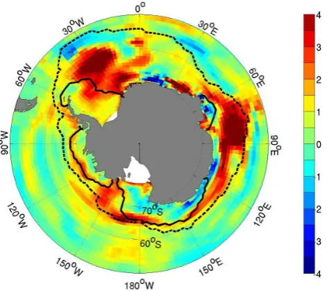
Except for the high latitude Southern Ocean, the effect of climate change in all other regions is generally not pro-nounced until the early 21st century. Less anthropogenic car-bon uptakes are simulated when climate change is included, predominantly in the Atlantic Ocean basin and in the Trop-ical and North Pacific Oceans. By 2099, in parts of the At-lantic Ocean, the model indicates a reduction of more than 0.2 Pg yr−1of anthropogenic carbon uptake, partly attributed to climate change. These negative changes (i.e., COU-UNC) in anthropogenic carbon uptake suggest positive climate-carbon cycle feedback mechanisms acting in most of the ocean regions. Nevertheless, Fig. 9 clearly indicates that the feedback strength could vary considerably from one region to another. In both polar regions (i.e., ARC and SOC), the COU simulates more carbon uptake than the UNC. This pattern im-plies that climate change increases the anthropogenic carbon uptake in these polar regions, particularly attributed to the sea ice retreat. By the end of the 21st century, the Southern Ocean would take up roughly∼0.15 Pg C yr−1 more when climate change is included in the model simulation. We note that the BCM-C model generates biases due to stronger mix-ing in this region, allowmix-ing the sea ice to almost disappear in the summer period. Figure 10 shows that most of the dif-ference between carbon uptake in the COU and UNC simu-lations occurs within or close to the areas where the sea ice has retreated. The retreat of sea ice due to melting allows an additional uptake of approximately 20 Pg carbon between years 2000 and 2099.
4.5.2 Climate impact on regional CO2flux determining
properties
In the next step, we analysed how regional climate change al-ters the oceanic carbon uptake mechanisms simulated in the BCM-C, particularly toward the end of the experimental peri-ods. In the model, the flux of carbon between the atmosphere and the ocean interface is defined as follows:
FCO2=α·K·1pCO2, (4)
whereαis the solubility of CO2gas in seawater computed as
a function of seawater temperature and salinity according to
Weiss (1974),Kis the gas transfer velocity, which depends on the surface wind speed and the Schmidt number according to Wanninkhof (1992) and1pCO2is the difference in partial
pressure of CO2between the atmosphere and the ocean. In
the model, solubility of gaseous CO2in seawater is
predom-inantly determined by SST and secondarily by surface salin-ity, where higher SST and higher salinity both lead to lower solubility. In contrast, lower SST and lower salinity lead to higher solubility. The CO2gas transfer velocity in the model
is mainly proportional to the fraction of sea-ice coverage and the square of surface wind speed, but it also depends on the SST. Thus, higher wind speeds and lower surface tempera-tures lead to a faster transfer rate of CO2gas into or out of
the ocean.
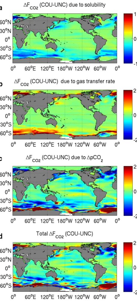
To first order, climate change (i.e., warming) affects the solubility and gas transfer rate. We computed the compara-tive change of these parameters (for the period 2080–2099) relative to the pre-industrial period (i.e., 1850–1869) for the COU simulations. Figure 11a shows that climate change re-duces the solubility in virtually all ocean regions. The largest reduction occurs within the high latitude oceans, where the solubility is reduced by approximately 20%, relative to the pre-industrial state. In parts of the North Atlantic sub-polar gyre, there is a slight increase in solubility due to the SST cooling in this region. Figure 11b shows that future climate change increases the gas transfer rate notably in the model, particularly in the polar regions. Here, the gas transfer rate increases by more than 100% due to the retreat in sea-ice. While solubility reduction leads to the decrease in carbon uptake, increase in gas transfer rate increases the carbon ex-change across the air-sea interface. For the UNC simulation, there is no significant change in the solubility and gas transfer rate. Both COU and UNC simulations generally yield simi-lar spatial change in1pCO2component of Eq. (4), as both
simulations apply the same atmospheric CO2concentration.
To quantitatively estimate how changes in each of the above parameters affect the regional carbon uptake, we ap-plied the similar method used by Crueger et al. (2008). Fol-lowing their study, differences in carbon uptake simulated by the COU and UNC can be approximately separated into differences due to solubility, gas transfer rate, and1pCO2
variation:
1FCO2(COU−UNC)≈1Fα+1FK+1F1pCO2, (5)
where1Fα, 1FK, and1F1pCO2 can be estimated as
fol-lows:
1Fα=1α·K·1pCO2, (6)
1FK=α·1K·1pCO2, (7)
1F1pCO2=α·K·1(1pCO2). (8)
0o 60oE 120oE 180oW 120oW 60oW 0o 60oS
30oS 0o 30oN 60oN
Integrated air−sea CO2 flux (1860−2099)
0 2 4 6 8
0o 60oE 120oE 180oW 120oW 60oW 0o 60oS
30oS 0o 30oN 60oN
a
b
Difference (COU−UNC) in integrated air−sea CO2 flux
−2 −1 0 1 2
Fig. 8. Map of (top) time-integrated (1860–2099) changes in carbon uptake relative to the pre-industrial period (1850–1859) from the COU
simulations and (bottom) the difference between the fully coupled and the uncoupled simulations (COU-UNC). Units are in [kg C/m2]
1850 1900 1950 2000 2050 2100 −0.2
−0.1 0 0.1 0.2
year
Annual carbon uptake difference [Pg C/yr]
SOC (>60S) NAT (20N−60N) TAT (20S−20N) SAT (20S−60S) NPA (20N−60N) TPA (20S−20N) SPA (20S−60S) TIN (20S−20N) SIN (20S−60S) ARC (>60N)
Fig. 9. Coupled minus uncoupled (COU-UNC) of spatially-integrated annual oceanic carbon uptake (10-year running mean). Regions
Fig. 10. Changes in atmospheric carbon uptake (similar to Fig. 8b)
for the Southern Ocean together with average winter (January 2070–2099) sea-ice extent for the (solid black line) COU and (dashed black line) UNC simulations. Unit of colour shades are in [kg C/m2]
0o 60oE 120oE 180oW 120oW 60oW 0o 60oS
30oS 0o 30oN 60oN
Relative change in solubility (2080−2099)−(1850−1869) [%]
−20 −10 0 10 20
0o 90oE 180oW 90oW 0o 0o 90oE 60oS
30oS 0o 30oN 60oN
a
b
Relative change in gas transfer rate (2080−2099)−(1850−1869) [%]−200 −100 0 100 200
Fig. 11. Change in CO2gas solubility and gas transfer rate for the
2080–2099 period relative to the pre-industrial period simulated in the COU. Units are in [%].
are performed for the difference and average for the period of 2080–2099, since the largest changes between the two simulations occur within this period (see also Fig. 9). Fi-gure 12 shows the map of changes of oceanic carbon uptake attributed to these different terms (based on Eqs. 6, 7, and
8) together with the actual difference of simulated carbon uptake between the two runs (i.e., left-hand side of Eq. 5). Positive values represent more carbon uptake when climate change is taken into consideration, whereas negative values represent less carbon uptake with climate change.
While the model simulates global warming of SST by approximately 2.5◦C, most of this warming occurs within high latitude regions (i.e., Southern Ocean, northwest Pa-cific, North Atlantic, and the Arctic), which leads to a reduc-tion of CO2solubility. In contrast, in the North Atlantic near
Greenland, there is a slight increase of solubility due to SST cooling. An earlier study, such as Mikolajewicz et al. (2007) also produced similar cooling in their future model simula-tion. We attribute this cooling of SST to the potential reduc-tion of lateral heat fluxes from the warm subtropical water in connection to the slowdown of AMOC strength. In the Southern Ocean, the reduction in the solubility pattern also reflects a pattern of SST increase caused by climate change. Maximum SST increases by as much as 5◦C are simulated along latitude 60◦S of the Indian and Atlantic Ocean sec-tions. Consequently, we see similar patterns in the reduction of carbon uptake due to lower solubility (see Fig. 12a). Con-sistent with the study by Crueger et al. (2008), our model produces smaller changes in surface solubility in the Equa-torial Pacific, despite a regional sea surface warming of up to 3◦C. To confirm this, we performed a simple back-of-the-envelope calculation of CO2gas solubility (Weiss, 1974) in
seawater using mean SST and SSS for the period 2080–2099 (29.4◦C, 34.5 psu) as compared to the pre-industrial period (26.8◦C, 34.6 psu). The calculation yielded a reduction of solubility from 0.0278 to 0.0262 moles L−1ppm−1. This rel-atively small change in solubility is due to the fact that the solubility changes are less significant in warmer than colder environments (Weiss, 1974).
An increase in carbon uptake due to increased gas trans-fer velocities predominantly occurs in the Southern Ocean along the 60◦S latitude band. Whilst there is an increase (i.e., by approximately 30%) in the zonal average near sur-face wind speed along 60◦S latitude, a significant increase in gas transfer velocity is mainly attributed to the retreat of the average sea ice from approximately 55◦S to>60◦S (see also Fig. 10). Also note that the HAMOCC5.1 model treats sea ice as an impermeable lid, thus, the fraction of sea ice in the model grid is a determining factor for air-sea gas exchange. Over the North Atlantic sub-polar gyre, there is a small re-duction in wind stress, which slightly reduces the carbon up-take in this region as shown in Fig. 12b.
Despite large spatial variabilities in the factors determin-ing regional carbon uptake mechanism, Fig. 12c and d show that differences in carbon uptake between the COU and UNC simulations mainly resemble the effect of changes in par-tial pressure CO2 difference between the atmosphere and
the ocean. Since the atmospheric CO2concentration in the
Fig. 12. Differences in oceanic carbon uptake between the COU
and UNC (2080–2099) due to the (a) solubility, (b) gas trans-fer velocity, (c) diftrans-ference in partial pressure of CO2effects, and
the (d) total simulated carbon uptake difference. Units are in [moles C m−2yr−1]. Positive values represent more carbon uptake when climate change is taken into consideration, whereas negative values represent the opposite.
spatial surface ocean pCO2 pattern. Surface pCO2 in the
model is controlled by surface DIC, alkalinity, salinity and temperature. The surface DIC concentration is, in turn,
60oE 120oE 180oW 120oW 60oW 60oE 120oE 60oS
30oS 0o 30oN 60oN
Changes in Revelle factor (2099−1850) COU
−0.4 −0.2 0 0.2 0.4
60oE 120oE 180oW 120oW 60oW 60oE 120oE 60oS
30oS 0o 30oN 60oN
Changes in Revelle factor (2099−1850) UNC
−0.4 −0.2 0 0.2 0.4
60oE 120oE 180oW 120oW 60oW 60oE 120oE 60oS
30oS 0o 30oN 60oN
a
b
c
Revelle factor change due to climate change (COU−UNC)−0.4 −0.2 0 0.2 0.4
Fig. 13. Difference in Revelle factors between year 2099 and 1850
simulated in the (a) COU and (b) UNC simulations, and (c) COU minus UNC for year 2099.
mined by regionally and temporally varying biophysical pro-cesses such as the ocean circulation, biological activity and convective mixing (Tjiputra and Winguth, 2008). In large portions of the low-latitude regions (30◦N–30◦S), there is little difference in the1pCO2between the COU and UNC
simulations. This suggests relatively small differences in the low-latitude ocean circulation and biological activity simu-lated in the COU and UNC. In the North Atlantic (between 30◦N–60◦N), the1pCO2simulated in the COU run is lower
than that of the UNC run. This difference is potentially due to weaker winter mixing processes (i.e., the average mixed-layer depth decreases by as much as 100 m in the simula-tion with climate change), which is the dominant mecha-nism for transporting CO2from the surface to the deep ocean
and maintaining lower surface DIC concentrations. In the North Pacific, noticeably lower carbon uptake due to lower
1pCO2 is simulated in COU. In contrast to the North
be the reason for lower1pCO2simulated in COU. Note that
warmer SSTs would yield higher partial pressures of CO2
despite similar surface DIC concentrations. Warming over the Southern Ocean between 30◦S and 60◦S lowers the ave-rage mixed-layer depth and increases the surfacepCO2 in
the COU. However, in regions where the warming causes the sea-ice cover to disappear (South of 60◦S), the model sim-ulates an increase of the average mixed layer depth, by as much as 100 m, as compared to the simulation without cli-mate change.
In terms of the global carbon budget, Fig. 12 also indicates that the consequences of climate change in the air-sea CO2
flux determining terms in the model are of the same order of magnitude. This suggests that the climate induced changes in CO2solubility, gas transfer rate, as well as1pCO2are of
equal importance in regulating the feedback mechanism. 4.5.3 Changes in regional Revelle factor
The above analysis shows that warming will reduce the solu-bility of CO2gas in seawater. However, we note that changes
in SST andpCO2will influence the Revelle factor. The
Rev-elle factor measures the changes of partial pressure of CO2
in seawater for a given change in DIC. Hence, for a given in-crease in atmospheric CO2concentration, ocean waters with
low values of the Revelle factor have higher oceanic equi-librium concentration of DIC than ocean waters with a high Revelle factor (Sabine et al., 2004). In this study, the simu-lated increase in water temperature will reduce the Revelle factor (i.e., increase the buffer capacity), through a better dissociation of CO2into bicarbonate and carbonate. On the
other hand, the Revelle factor increases with risingpCO2
(Zeebe and Wolf-Gladrow, 2001). In order to estimate the changes in Revelle factor due to climate change (i.e., increase in SST) as well as due to increase in surfacepCO2, we
com-pute the difference between the Revelle factor for year 2099 and year 1850 from the COU and UNC simulation, as shown in Fig. 13a and b. The Revelle factor is estimated using the formulation from Maier-Reimer and Hasselmann (1987). Generally, there is an agreement in increasing Revelle fac-tor in the future, hence, lower buffer capacity of seawater to take up CO2. For most regions, Fig. 13b resembles well the
spatial pattern of Fig. 13a (i.e., higher values in high latitude and relatively small changes in low latitude). The similar-ity between the Revelle factor changes simulated in the COU and UNC suggests that changes in surfacepCO2(instead of
climate change) may dominate the future Revelle factor vari-ation. In several high latitude regions, such as northwestern Pacific and the Southern Ocean (south of 60◦S), the simu-lated warming in SST of as much as 5◦C maintain the Rev-elle factor similar or lower than that of the pre-industrial pe-riod. In addition, we can estimate the future changes of the Revelle factor attributed to only climate change by comput-ing the difference in Revelle factor between the COU and UNC simulations for year 2099 (shown in Fig. 13c).
Fi-gure 13c demonstrates that warming in parts of the Southern Ocean and northwestern Pacific induces lower Revelle factor. On the other hand, cooling in the North Atlantic sub-polar gyre slightly increases the Revelle factor in that region.
5 Discussion and conclusions
In this study, we coupled terrestrial (LPJ) and oceanic (HAMOCC5) global carbon cycle modules into the Bergen Climate Model (BCM). Our results show that the BCM-C model is able to simulate relatively well the temporal and spatial variabilities of the observed present climate and car-bon cycle processes. The simulated future projection of at-mospheric CO2concentration as well as global oceanic and
terrestrial carbon uptake lies well within range of other Earth system models. Nevertheless, we note that the current model does not allow the terrestrial vegetation to feedback to the atmosphere by changing the surface albedo. The model also ignores the terrestrial nitrogen cycle and the spatial variabil-ity of atmospheric CO2concentrations.
The fully coupled climate-carbon cycle model (BCM-C) is integrated for the period 1850–2100 and forced by pre-scribed historical and IPCC SRES-A2 CO2 emission
sce-narios. In order to assess the mechanisms controlling the climate-carbon cycle feedback, two model simulations were generated, one where the climate change effect is included and one where it is suppressed. According to previous stud-ies using complex three-dimensional Earth system models (Cox et al., 2000; Friedlingstein et al., 2006; Mikolajewicz et al., 2007), it is well accepted that future climate change is likely to reduce carbon uptake, retaining a larger frac-tion of airborne CO2 in the atmosphere. Our model
simu-lations also show a decrease in the strength of carbon uptake, predominantly by the terrestrial reservoir, despite a continu-ous oceanic carbon uptake towards the end of the 21st cen-tury. Nevertheless, previous feedback evaluations are mostly based on global assessments of the ocean and terrestrial reservoirs’ ability in storing carbon in relation to changes in global atmospheric CO2concentration and climate.
There-fore, the regional effect of carbon cycling on climate vari-ability and their controlling mechanisms remain poorly un-derstood. In this study, we further analyzed the processes controlling the climate-carbon cycle feedbacks strength in different regions.
Over land, climate change mostly impacts the tropical and northern high latitude regions. While an increase in ambient CO2 concentrations stimulates net primary production and
increases carbon storage in plant tissues, the consequences of warming generally lead to an increase in terrestrial soil respiration, and thus, induce carbon outgassing. The tropical regions respond most strongly to changes in the atmospheric CO2 concentrations because plant assimilation of CO2 is
turnover time, predominantly at high latitudes where the change in surface temperatures is at a maximum.
In this study, the dynamical vegetation schemes improve the climate-carbon cycle feedback estimate since it allows the PFTs (i.e., Plant Functional Type) to respond to warmer climate. Nevertheless, a more realistic estimation of the ter-restrial biosphere feedback requires the inclusion of land-use changes, whose impact is expected to be in the same order of magnitude as that of the vegetation regime shifts.
Unlike the terrestrial carbon cycle, there is relatively less change in the simulated global carbon uptake by the ocean between the COU and UNC. Regional analysis indicates that different processes in different parts of the world ocean con-tribute to dampen the relatively small carbon uptake changes between the two simulations. In addition, the consequences of climate change on ocean carbon uptake are not clearly ap-parent until the second half of this century.
Our study shows that there are both direct and indirect ef-fects of climate change in altering oceanic carbon uptake. The direct effects include an increase in SST, which di-rectly decreases the CO2 gas solubility in seawater, most
pronounced in high-latitude regions. While increase in SST could also lead to a reduced Revelle factor (i.e., better CO2buffer capacity), our analysis shows that the simulated
changes in Revelle factor are mostly dominated by changes in surfacepCO2, rather than SST. Additionally, changes in
atmospheric circulation (i.e., surface wind stress) tend to en-hance the transfer rate of carbon across the air-sea interface, also most pronounced in high-latitude regions, especially in regions where the sea ice retreats. On average, changes in solubility and gas transfer rate of CO2 alone would tend to
decrease and increase carbon uptake by the ocean, respec-tively.
The indirect effects of climate change include, but are not limited to, changes in ocean circulation dynamics, mixed layer depth, sea-ice extent and fresh water fluxes. These in-direct climate change factors significantly affect the high lat-itude Southern Ocean region. The summer sea ice extent in Antarctica, as simulated by the model, reduces almost to zero due to warming. This retreat of sea ice induces stronger CO2
gas transfer and deeper mixed layers, which in turn increase the transfer of carbon from the atmosphere to the ocean as well as from the surface into larger depths. A similar re-sponse to indirect effects of climate change is also shown in the Arctic region, where the model simulates a reduction of
∼25% in sea ice extent. Over most of the North Atlantic regions, warming leads to shallowing of mixed layer depths and a slowdown of the overturning circulation, which favours the reduction of the vertical transport of surface DIC into deeper layers.
Acknowledgements. The authors would like to thank
Mar-tin Miles, Andy Ridgwell, and the anonymous referees for thoroughly reviewing the manuscript. We are also very grateful to Pierre Friedlingstein and the C4MIP group for the support
and access to the original C4MIP data (used in Figs. 3 and 5). This study at the University of Bergen and Bjerknes Centre for Climate Research is supported by the EU-FP6 integrated project CarboOcean (grant nr. 511176), the Research Council of Norway funded project NorClim and CarboSeason (grant nr. 185105/530). We acknowledge the Norwegian Metacenter for Computational Science and Storage Infrastructure (NOTUR and NorStore, “Biogeochemical Earth system modelling” project nn2980k and ns2980k) for providing the computing and storing resources essential for this study. This is publication no. A266 from the Bjerknes Centre for Climate Research.
Edited by: A. Ridgwell
References
Assmann, K. M., Bentsen, M., Segschneider, J., and Heinze, C.: An isopycnic ocean carbon cycle model, Geosci. Model Dev. Dis-cuss., 2, 1023–1079, 2009.
Aumont, O., Maier-Reimer, E., Blain, S., and Monfray, P.: An ecosystem model of the global ocean including Fe, Si, P colimitations, Global Biogeochem. Cy., 17, 1060, doi:10.1029/2001GB001745, 2003.
Bleck, R., Rooth, C., Hu, D., and Smith, L. T.: Salinity-driven ther-mocline transients in a wind- and thermohaline-forced Isopycnic Coordinate Model of the North Atlantic, J. Phys. Oceanogr., 22, 1486–1505, 1992.
Bossuet, C., D´equ´e, M., and Cariolle, D.: Impact of a simple pa-rameterization of convective gravity-wave drag in a stratosphere-troposphere general circulation model and its sensitivity to verti-cal resolution, Ann. Geophys., 16, 238–249, 1998,
http://www.ann-geophys.net/16/238/1998/.
Catry, B., Geleyn, J.-F., Bouyssel, F., Cedilnik, J., Brozkova, R., Derkova, M., and Mladek, R.: A new sub-grid scale lift for- mu-lation in a mountain drag parameterisation scheme, Meteorol. Z., 17, 193–208, 2008.
Cox, P. M., Betts, R. A., Jones, C. D., Spall, S. A., and Totterdell, I. J.: Acceleration of global warming due to carbon cycle feedback in a coupled climate model, Nature, 408, 184–188, 2000. Cramer, W., Bondeau, A., Woodward, F. I., Prentice, I. C., Betts,
R. A., Brovkin, V., Cox, P. M., Fisher, V., Foley, J. A., Friend, A. D., Kucharik, C., Lomas, M. R., Ramankutty, N., Sitch, S., Smith, B., White, A., and Young-Molling, C.: Global response of terrestrial ecosystem structure and function to CO2and
cli-mate change: results from six dynamic global vegetation models, Glob. Change Biol., 7, 357–373, 2001.
Crueger, T., Roeckner, E., Raddatz, T., Schnur, R., and Wet-zel, P.:Ocean dynamics determine the response of oceanic CO2 uptake to climate change, Clim. Dynam., 31, 151–168,
doi:10.1007/s00382-007-0342-x, 2008.
de Szoeke, R. A.: Equation of motion using thermodynamic coor-dinates, J. Phys. Oceanogr., 29, 2719–2729, 2000.
D´equ´e, M., Dreveton, C., Braun, A., and Cariolle, D.: The ARPEGE/IFS atmosphere model: A contribution to the French community climate modelling, Clim. Dynam., 12, 37–52, 1994. Douville, H., Royer, J. F., and Mahfouf, J. F.: A new snow
![Fig. 6. Geographical distribution of accumulated carbon uptake by the land [Pg C] (top) simulated by the COU simulation and (bottom) thedifference between COU and UNC simulations](https://thumb-us.123doks.com/thumbv2/123dok_us/9117546.1904601/10.595.131.466.63.345/geographical-distribution-accumulated-carbon-simulated-simulation-thedifference-simulations.webp)