Complementing thermosteric sea level rise estimates

(1)

www.geosci-model-dev.net/8/2723/2015/ doi:10.5194/gmd-8-2723-2015

Complementing thermosteric sea level rise estimates

K. Lorbacher1, A. Nauels1, and M. Meinshausen1,2

1_{Australian-German College of Climate & Energy Transitions, School of Earth Sciences, The University of Melbourne,} Parkville 3010, Victoria, Australia

2_{The Potsdam Institute for Climate Impact Research, Telegrafenberg A26, 14412 Potsdam, Germany}

Correspondence to: K. Lorbacher (katja.dommenget@unimelb.edu.au)

Received: 9 December 2014 – Published in Geosci. Model Dev. Discuss.: 10 February 2015 Revised: 1 June 2015 – Accepted: 11 August 2015 – Published: 2 September 2015

Abstract. Thermal expansion of seawater has been one of the most important contributors to global sea level rise (SLR) over the past 100 years. Yet, observational estimates of this volumetric response of the world’s oceans to temperature changes are sparse and mostly limited to the ocean’s up-per 700 m. Furthermore, only a part of the available climate model data is sufficiently diagnosed to complete our quan-titative understanding of thermosteric SLR (thSLR). Here, we extend the available set of thSLR diagnostics from the Coupled Model Intercomparison Project Phase 5 (CMIP5), analyze those model results in order to complement upper-ocean observations and enable the development of surro-gate techniques to project thSLR using vertical tempera-ture profile and ocean heat uptake time series. Specifically, based on CMIP5 temperature and salinity data, we provide a compilation of thermal expansion time series that com-prise 30 % more simulations than currently published within CMIP5. We find that 21st century thSLR estimates derived solely based on observational estimates from the upper 700 m (2000 m) would have to be multiplied by a factor of 1.39 (1.17) with 90 % uncertainty ranges of 1.24 to 1.58 (1.05 to 1.31) in order to account for thSLR contributions from deeper levels. Half (50 %) of the multi-model total expan-sion originates from depths below 490±90 m, with the range indicating scenario-to-scenario variations. To support the de-velopment of surrogate methods to project thermal expan-sion, we calibrate two simplified parameterizations against CMIP5 estimates of thSLR: one parameterization is suitable for scenarios where hemispheric ocean temperature profiles are available, the other, where only the total ocean heat up-take is known (goodness of fit:±5 and±9 %, respectively).

1 Introduction

(2)

Aside from thermal expansion, SLR is also induced by changes in ice-sheet as well as glacier mass and land wa-ter storage that combined amounts to 60 % of the observed global mean SLR over 1971–2010 (Church et al., 2013a). Over the last century, these mass changes in the ocean (termed “barystatic” sea level changes by Gregory et al., 2013a) together with ocean’s thermal expansion have been the main contributors to global mean SLR. Some other influ-ences, such as salinity variations associated with freshwater tendencies at the sea surface and redistributed in the ocean’s interior have a negligible effect on seawater density and thus sea level changes on the global scale (e.g., Lowe and Gre-gory, 2006); on regional to basin scales, however, the role of salinity should not be neglected in sea level studies (e.g., Durack et al., 2014a). In the long term, the mass contribu-tion might become substantially larger than thermal expan-sion contribution to SLR because of the larger efficiency of land-ice melting for a given amount of heat (Trenberth and Fasullo, 2010). However, the current climate models of the Coupled Model Intercomparison Project Phase 5 (CMIP5) do not include land ice-sheet discharge dynamics and their contributions to the global mean SLR budget (Church et al., 2013b). Furthermore, simulating land ice-sheet discharge dy-namics from the Antarctic ice sheets might translate into large uncertainties in climate models, since non-linear pro-cesses may be triggered that could alter the sea level rise contribution dramatically (e.g., Joughin et al., 2014; Rignot et al., 2014; Mengel and Levermann, 2014). Since the be-ginning of the satellite altimetry era in 1993, the contribu-tion of thermal expansion to global mean SLR is estimated to be 34 % (observations) and 47 % (simulations), respec-tively (see Table 13.1 in Church et al., 2013a). Down to the present day, the observed SLR contribution from thermal ex-pansion is limited in the space and time dimension: available observed long-term (decadal) time series of thermosteric sea level rise (thSLR) are mainly globally averaged values using different spatio-temporal interpolation/reconstruction meth-ods and cover the upper 2000 m at maximum (Domingues et al., 2008; Ishii and Kimoto, 2009; Levitus et al., 2012). Observed contributions to thSLR from depths below 2000 m are assumed to increase monotonically and linearly in time (Purkey and Johnson, 2010; Kouketsu et al., 2011). For de-tails on the spatial as well as temporal coverage and quality of oceanic temperature measurements that underlie thSLR estimates we refer to Abraham et al. (2013) and references therein.

The objective of the present study is both to complement observed and existing simulated thSLR estimates in a num-ber of ways and to enable the development of surrogate tech-niques for long-term thSLR projections. We begin by intro-ducing the observed and simulated data sets as well as the method to arrive at thSLR estimates. Subsequently, we cal-culate the simulated thermal expansion over the entire ocean grid for a number of CMIP5 models that have not published those time series yet. Sections 3 and 4 present both the

ex-tended CMIP5 thSLR (zostoga) data set and depth-dependent results that can complement upper ocean layer observations. Sections 5 and 6 investigate hemispheric and global averages of calibrated thSLR mimicking CMIP5 estimates. In Sect. 7 we discuss and summarize our results focussing on the extent to which the observations might underestimate the contribu-tion to thSLR from depths below the main thermocline.

2 Methods and models

The volumetric response to changes in the ocean’s heat bud-get, the thermosteric sea level, η2, at any horizontal grid point and any arbitrary time step is defined by the verti-cally integrated product of the thermal expansion coefficient, α, and the potential temperature deviation from a reference state,2exp−2ref,

η2(x, y, t )= 0 Z

−H

α(2exp−2ref)dz, (1)

where the spatial 3-D thermal expansion coefficient,αis de-fined by

α= −1

ρ(Sref, 2ref, p)

ρ(Sref, 2exp, p)−ρ(Sref, 2ref, p)

(2exp−2ref)

. (2) CMIP5 publishes time series of global mean (0-D)η2, called zostoga and represents the integral value of ocean’s thermal

expansion,α(2exp−2ref), at each grid point, over the entire

ocean volume. For the majority of the fully coupled climate models, sea level changes due to net gain of heat need to be diagnosed offline as a result of using the Boussinesq approx-imation, conserving ocean’s volume and not mass (Great-batch, 1994). Here, we derive global mean yearly depth pro-files of thermal expansion by using independent2 and S prognostics of CMIP5 model simulations in Eq. (2).

In order to derive thermal expansion estimates, and

zos-toga, from hemispherically or globally averaged vertical

tem-perature profiles, rather than from sparsely observed and computationally expensive spatial 3-D fields of temperature, salinity and pressure, we use a simplified parameterization of a thermal expansion coefficient,α1.5, as a polynomial of2 andp:

α1.5=(c0+c120(12.9635−1.0833p) −c221(0.1713−0.019263p)

(3)

1996; Wigley et al., 2009; Meinshausen et al., 2011). The depth profile, z, is expressed by the pressure profile p= 0.0098(0.1005z+10.5exp((−1.0)z/3500)−1.0), assuming a mean ocean depth of 3500 m and a mean maximum ocean depth of 6000 m in Eq. (3). As a first step, we use time-dependent vertical global and hemispheric profiles of2from the CMIP5 models to test the reliability of thermal expansion estimates based on this simplified approach (Eq. 3). With these time series of vertical temperature profiles we calibrate α1.5in Eq. (3) with calibration parameterscnagainst globally and hemispherically averaged vertical profiles ofαin Eq. (2) (using squared differences as goodness-of-fit statistic).

We name this parameterization the 1.5-D simplification, as it uses two hemispherically averaged depth profiles. In addi-tion, we use the CMIP5 data to estimate the zero-dimensional (0-D) thermal expansion coefficientα0. Divided by ocean’s specific heat capacity, reference density and area, it gives the “expansion efficiency of heat” (in m YJ−1_{, 1 YJ}_≡₁₀24_J) and allows the comparison of thermal expansion from mod-els with different spatial dimensions (Russell et al., 2000). This constant quantifies the proportionality between global mean thSLR and ocean heat uptake (OHU) (cf. Kuhlbrodt and Gregory, 2012).

We examine a broad range of CMIP5 scenarios, namely the historical (post-1850) climate simulations, the idealized 1 % CO2 per year increase (1pctCO2) and the response to abrupt 4× pre-industrial CO2 increase (abrupt4xCO2). But as we aim to complement observed and existing sim-ulated thSLR estimates and to design surrogate techniques to project long-term thSLR, we focus on the four sce-narios defining future change in radiative forcing, namely

rcp2.6, rcp4.5, rcp6.0 and rcp8.5. These scenarios specify

four greenhouse gas concentration trajectories and their Rep-resentative Concentration Pathways (RCP). They are named after the amount of radiative forcing (in W m−2) realized in the year 2100 relative to values of the pre-industrial (pre-1850) control scenario (piControl) (for details see Taylor et al., 2012; Moss et al., 2010, and Table S1 in the Sup-plement). However, recent literature suggests that the rapid adjustment primarily due to clouds generates forcing varia-tions that cause differences in the projected surface warming among the CMIP5 models even if radiative forcing is equally prescribed for each individual CMIP5 model (Forster et al., 2013).

Independent of the model and estimation method, a “full linear drift” is removed from all simulated thermosteric sea level time series, zostoga and temperature time series by sub-tracting a linear trend based on the entire corresponding

(pi-Control) scenario in order to allow for comparison with

ob-servational time series. For our globally and hemispherically averaged thSLR time series the sensitivity to the method of drift correction is less than 1% due to small low-frequency (inter-annual to inter-decadal) variability present in the evo-lution of this integral oceanic property. This contrasts the large low-frequency variability, e.g. in the sea surface

tem-perature evolution (Palmer et al., 2009). For details about methods of climate drift correction in CMIP5 models see Taylor et al. (2012), Sen Gupta et al. (2013) and the sup-plementary by Church et al. (2013a). Additionally, we cor-rect the historical time series by adding the suggested thSLR trend of 0.1±0.05 mm yr−1by Church et al. (2013b) to take into account that the CMIP5 piControl scenario might be conducted without volcanic forcing and thus underestimate the oceanic thermal expansion in the historical scenario (Gre-gory et al., 2013b). The adjustment of global mean SLR to changes in ocean mass is fast and linear (Lorbacher et al., 2012); thus in the longer term, impacts of changing ocean mass on SLR may well become the primary contribution to the trend in SLR. For projected time series beyond the his-torical simulations, we use the rcp4.5 simulations consistent with Church et al. (2013a).

3 Extended CMIP5zostogadata set

For CMIP5 models that report zostoga, we calculate the RMSE between published zostoga values and our recalcu-lated values based on the provided 2 and initial S depth profiles. Averaged over all CMIP5 models and scenarios and normalized by the mean zostoga value, the RMS-error amounts to±1 %, providing confidence that our 3-D equa-tion of state implementaequa-tion is consistent with those of CMIP5 modelling groups. As not all CMIP5 models that provide 2 and S also provide zostoga, our recalculated data set comprises 30 % more modelled zostoga time se-ries than currently published within CMIP5 (compare Ta-ble S1 and Fig. 1a, e.g., to Fig. 13.8 in Church et al., 2013a). These complementing zostoga time series contribute 50 % more CMIP5 models to multi-model ensemble thSLR estimates than previously used by Church et al. (2013a); they are available at http://climate-energy-college.net/ complementing-thermosteric-sea-level-rise-estimates and as Supplement. Time series of zostoga published by the individ-ual model groups are available, e.g., here http://pcmdi9.llnl. gov/esgf-web-fe.

(4)

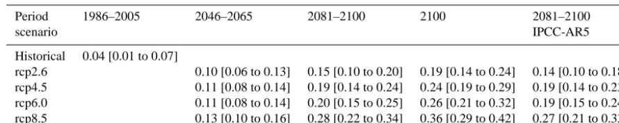
Table 1. Median and its 90 % confidence interval for projections of global mean thSLR (in m) in 2046–2065 and 2081–2100 relative to

1986–2005 as well as in year 2100 relative to year 1900 for the four RCP scenarios.

Period 1986–2005 2046–2065 2081–2100 2100 2081–2100

scenario IPCC-AR5

Historical 0.04 [0.01 to 0.07]

rcp2.6 0.10 [0.06 to 0.13] 0.15 [0.10 to 0.20] 0.19 [0.14 to 0.24] 0.14 [0.10 to 0.18]

rcp4.5 0.11 [0.08 to 0.14] 0.19 [0.14 to 0.24] 0.24 [0.19 to 0.29] 0.19 [0.14 to 0.23]

rcp6.0 0.11 [0.08 to 0.14] 0.20 [0.15 to 0.25] 0.26 [0.21 to 0.32] 0.19 [0.15 to 0.24]

rcp8.5 0.13 [0.10 to 0.16] 0.28 [0.22 to 0.34] 0.36 [0.29 to 0.42] 0.27 [0.21 to 0.33]

4 Complementing observations

For the upper 700 m, our extended CMIP5 multi-model median rate of thSLR and its standard deviation globally amounts to 0.57±0.03 mm yr−1_{from 1971 onward to 2010} (Figs. 1b and S3b in the Supplement) and is similar to the observed arithmetic mean 0.53±0.02 mm yr−1 of the three individual trends 0.63±0.02 mm yr−1 (Domingues et al., 2008), 0.45±0.02 mm yr−1 (Ishii and Kimoto, 2009) and 0.50±0.03 mm yr−1 (Levitus et al., 2012) (cf. Fig. 13.4 in Church et al., 2013a). For the same period, around half of the models underestimate the ocean’s thermal expansion in sim-ulations, even after the correction for missing volcanic forc-ing in the piControl scenario (Gregory et al., 2013b). Never-theless, the majority of the historical scenarios capture the main volcanic eruptions in the years 1963 (Agung), 1982 (El Chichón) and 1991 (Pinatubo) with a sea level drop 1– 2 years later. Generally, differences in the observed and in-terannual variability suggest that the underlying spatial pat-terns of interannual thermosteric sea level variability are dif-ferent (Fyfe et al., 2010). For the altimetry period (1993– 2010), our multi-model median is 1.45 mm yr−1, with 1.02 to 1.97 mm yr−1as 90 % uncertainty, taking into account the contribution of thermal expansion to the global mean SLR from the entire ocean depth. This rate of thSLR equals the corresponding rate of 1.49 mm yr−1and its uncertainty range of 0.97 to 2.02 mm yr−1 listed in Table 13.1 by Church et al. (2013a) and confirms again the robustness of simulated thSLR estimated presented by Church et al. (2013a) with 30 % less models for a multi-model estimate than used here. The model median contribution to thSLR from the layer between 700 and 2000 m suggests a slight underestimation of the observational data for the period 2005–2013 (Figs. 1c and S3c). For ocean depths below 2000 m, the model median trend for the years 1990–2000 of 0.11 mm yr−1_{in the} histor-ical scenario seems to reliably represent the thSLR contribu-tion which Purkey and Johnson (2010) estimated (Figs. 1d and S3d). For an ocean warming occurring at a depth below 3000 m Kouketsu et al. (2011) estimate a similar thSLR over a 40-year period; based on observed and assimilated data it amounts to 0.10 and 0.13 mm yr−1, respectively. For the upper 2000 m, the depth profiles of thermodynamic proper-ties across CMIP5 models are largely aligned with

observa-tional depths profiles for2andSof the modern day (2005– 2013) ocean provided by the Argo program (Roemmich and Gilson, 2009); the same is true for the derived thermal ex-pansion coefficient (see Fig. 2 and depth profiles of poten-tial temperatures in the piControl scenario by Kuhlbrodt and Gregory, 2012). The simulated salinity profile shows the ob-served maximum at around 200 m that reflects evaporation zones and a minimum at around 500 m that reflects mode water regions. For depths below 500 m, the model spread of 2 andS amounts to 2◦C and 0.4 PSS-78, with only a few model outliers. Independent of the model and scenario, the thermal expansion coefficient α at the sea surface de-creases from 4×10−4◦C−1in tropical to near zero in polar regions and, globally averaged, shows the familiar concave vertical profile (e.g., Griffies et al., 2014) with a minimum around 1500 m (Fig. 2). The minimum global mean clima-tological value ofαamounts to 1.3×10−4◦C−1for the his-torical scenario and agrees well with the observed one. Av-eraged over the entire water column,α(1.56×10−4◦C−1) compares well with the corresponding value from ocean-only simulations (1.54×10−4◦_C−1_{, Griffies et al., 2014). In the} Northern Hemisphere,αis 1 % higher than in the Southern Hemisphere because average temperatures tend to be higher above 2000 m in the Northern Hemisphere (not shown). For details on the horizontal and vertical behaviour ofαsee, e.g., Griffies et al. (2014) and Palter et al. (2014).

(5)

1850 1900 1950 2000 2050 2100 time (in years)

0.0 0.2 0.4 0.6 0.8

thermosteric sea level rise (in m)

(a/) total historical 1pctCO2 abrupt4xCO2 rcp2.6 rcp4.5 rcp6.0 rcp8.5

1950 1960 1970 1980 1990 2000 2010 2020

time (in years)

1.5 1.0 0.5 0.0 0.5 1.0 1.5 2.0 2.5

thermosteric sea level rise (in cm)

Pinatubo

Agung El Chichon (b/) upper 700 m

Domingues et al. (2008) Ishii and Kimoto (2009) Levitus et al. (2012) historical+rcp4.5

1990 1995 2000 2005 2010 2015 2020

time (in years)

0.5 0.0 0.5 1.0 1.5

(c/) 700-2000 m

Roemmich and Gilson (2009) Levitus et al. (2012) historical+rcp4.5

1990 1995 2000 2005 2010 2015 2020

time (in years)

0.5 0.0 0.5 1.0 1.5

(d/) below 2000 m Purkey and Johnson (2010) historical+rcp4.5

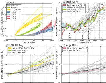
Figure 1. Time series of observed and simulated global mean yearly thSLR (in cm). (a) Simulated thSLR (zostoga) relative to year 1900 for

seven CMIP5 scenarios: historical (31/47), 1pctCO2 (19/32), abrupt4xCO2 (17/30), rcp2.6 (18/26), rcp4.5 (27/40), rcp6.0 (13/20), rcp8.5 (27/40); the ratio in brackets indicates the number of models of published (solid lines) zostoga and recalculated (dashed lines) zostoga in this study based on simulated temperature and salinity fields. Bars indicate the thSLR of the four RCP scenarios in year 2100 (see also Table 1). (b) Observed contribution to yearly thermosteric sea level of the upper 700 m by Domingues et al. (2008), Ishii and Kimoto (2009) and Levitus et al. (2012) relative to year 1961 and corresponding simulated time series of the historical and rcp4.5 scenarios, whereby the solid light (dark) grey lines represent the model mean (median). Observed contribution to yearly thermosteric sea level (in cm) from layers

(c) between 700 and 2000 m by Levitus et al. (2012) and Roemmich and Gilson (2009) and (d) below 2000 m by Purkey and Johnson (2010)

relative to year 1993 (indicating the start of the satellite sea level altimetry period). Corresponding simulated time series are shown as in (b).

2000 m (as share of total thSLR) shows an opposing trend compared to the 21st century evolution of the multi-gas sce-narios. Firstly, the idealized experiments are started from pre-industrial control equilibrium conditions and hence miss the initial stratification and upper layer expansion between

his-torical’s start year (usually 1850) and the start year of our

analysis (1900 for the historical and 2006 for the RCP sce-narios) (cf. Russell et al., 2000). Secondly, the initial warm-ing pulse in abrupt4xCO2 is extreme: already within the first year of the model scenario, thermal expansion in the up-per 300 m shows a clear increase in the global mean, for all CMIP5 models, and amounts to a magnitude of thermal ex-pansion corresponding to the last 20 years (1986–2005) of the historical scenario (Figs. 2d, h and S3a). After 20 years, the thermal expansion for the abrupt4xCO2 scenario in this upper layer equals almost the thermal expansion of the rcp2.6 scenario at the end of the 21st century (not shown). Both characteristics of abrupt4xCO2 define a large vertical tem-perature gradient between surface and deeper water almost

(6)

0 5 10 15 20 potential temperature (in degC) 0

1000

2000

3000

4000

5000

6000

7000

depth (in m)

(a/)

Roemmich and Gilson (2009) FGOALS-g2 GISS-E2-H GISS-E2-R GISS-E2-R-CC

32.0 32.5 33.0 33.5 34.0 34.5 35.0 35.5 36.0 salinity (in psu) (b/)

1.0 1.2 1.4 1.6 1.8 2.0 2.2 2.4 2.6 2.8 thermal expansion coefficient (in 1.e-4/degC)

(c/)

0.10 0.05 0.00 0.05 0.10 0.15 0.20 thermal expansion (in mm/m) (d/)

1 0 1 2 3 4 5

potential temperature deviation (in degC) 0

1000

2000

3000

4000

5000

6000

7000

depth (in m)

(e/)

0.2 0.0 0.2 0.4 0.6 0.8 1.0 1.2 thermal expansion (in mm/m) (f/)

1.0 1.2 1.4 1.6 1.8 2.0 2.2 2.4 2.6 2.8 thermal expansion coefficient (in 1.e-4/degC)

(g/)

0.10 0.05 0.00 0.05 0.10 0.15 0.20 thermal expansion (in mm/m) (h/)

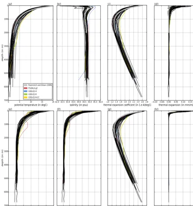
Figure 2. Global mean vertical profiles for all models of historical in year 1900 (upper panels, a–c), historical in year 2005 relative to year

1986 (d), rcp8.5 in year 2100 relative to the historical mean over 1986 to 2005 (lower panels, e–g) and abrupt4xCO2 within the first year (h):

(a) potential temperature (in◦C, 0 to 20), (b) salinity (in PSS-78, 32 to 36) and (c) thermal expansion coefficientα(in 10−4◦C−1, 1.2 to 2.8); (d) thermal expansion per layer (in mm m−1,−0.1 to 0.2), (e) temperature deviation (in◦C,−1 to 5), (f) thermal expansion per layer (in mm m−1,−0.2 to 1.2) and (g) thermal expansion coefficientα(in 10−4◦C−1, 1.0 to 2.8), (h) thermal expansion per layer (in mm m−1,

−0.2 to 1.2). Observed profiles (grey lines) are based on the Argo data as an average over the period 2005 to 2013, except for the thermal expansion in (d). Model outliers are indicated in (a).

i.e., the start of the RCP scenarios, the volcanic forcing in historical might suppress the thermal expansion of middle layers (700–2000 m) and might therefore lead to a certain rebound effect of the middle layer thSLR contributions in the mid-21st century (cf. Fig. S3). However, for the multi-gas scenarios, the overall 21st century multi-model median thSLR contribution of the deep ocean is 39% from depth be-low 700 m with 24 to 58 % as 90 % uncertainty and 17 % from depths below 2000 m with 5 to 31 % as 90 % uncer-tainty (see Fig. 3a–d). The contributions for the RCP

refer-ence period (1986–2005, Church et al., 2013a) taken from the historical simulations are 46 % [21 to 73 %] (and 21 % [4 to 44 %]) (Fig. 3e).

5 The 1.5-D parameterization

(7)

2020 2040 2060 2080 2100

time (in years)

0 10 20 30 40 50 60 70 80

contribution to total thermosteric sea level (in %)

22 64 33 49 40 4 40 12 23 19 22 45 30 41 36 5 27 9 18 14 22 57 28 40 33 2 22 7 15 10 (a/) rcp8.5

below 700 m below 2000 m

2020 2040 2060 2080 2100

time (in years)

0 10 20 30 40 50 60 70 80 22 60 37 47 41 5 38 12 28 20 25 59 32 47 39 5 31 11 22 18 27 59 32 45 38 4 28 9 20 13 (b/) rcp6.0

2020 2040 2060 2080 2100

time (in years)

0 10 20 30 40 50 60 70 80 23 64 34 48 41 5 37 13 24 20 26 62 33 45 39 5 33 11 22 15 27 65 34 47 41 3 29 9 20 13 (c/) rcp4.5

2020 2040 2060 2080 2100

time (in years)

0 10 20 30 40 50 60 70 80 20 60 32 44 39 5 35 13 25 21 24 64 34 48 40 5 33 13 23 19 30 69 36 53 45 5 36 12 24 15 (d/) rcp2.6

1900 1920 1940 1960 1980 2000

time (in years)

0 20 40 60 80 100

contribution to total thermosteric sea level (in %)

18

83

35

57

47

6

60

15

35

24

28

79

40

56

48

10

49

19

31

23 ₂₁

73

37

56

46

4

44

15

30

21 median

mean

75%

25%

95%

5%

(e/) historical

1900 1920 1940 1960 1980 2000

time (in years)

0 10 20 30 40 50 60 70 80 10 42 15 28 24 5 24 7 17 11 14 39 21 29 26 3 18 8 13 11 19 45 25 35 29 2 19 7 13 9 (f/) 1pctCO2

1900 1920 1940 1960 1980 2000

time (in years)

0 10 20 30 40 50 60 70 80 4 12 6 10 8 1 6 243 12 29 18 26 22 1 13 4 8 5 19 54 27 38 33 2 16 6 10 7 (g/) abrupt4xCO2

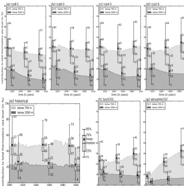
Figure 3. Model median percentage contribution to global mean thSLR for the entire water column from depths below 700 m (light grey) and

below 2000 m (dark grey) for the historical scenario, for projections for the four RCP scenarios and the two idealized CO₂scenarios derived from Eq. (2). Whisker plots quantify the temporal average distribution of the contribution to thSLR of the first 20 years, the entire time series and the last 20 years, respectively: 2006–2025/2006–2100/2081–2100 for RCPs (a–d); 1901–1920/1900–2005/1981–2005 for the historical scenario (e); and 1–20/1–100/81–100 for the 1pctCO2 and abrupt4xCO scenarios (f, g). Bars and whiskers represent the 25–75 and 5–95 % uncertainties of the median, respectively; the central mark of the bar indicates the model median, the asterisk the model mean.

the thSLR time series obtained by using potential temper-atures and standard pressure profiles with Eq. (3), we then obtain an average error of ±5 %, ranging between 1 and 17 % across the CMIP5 model suite (see Table S2). The hemispherically averaged percentage contributions to thSLR based on the 1.5-D simplified thermal expansion coefficient (Eq. 3) for all seven scenarios compare well with our ex-tended CMIP5 data set (Fig. 4). The thSLR contribution from depths below 2000 m is larger in the Southern Hemi-sphere than in the Northern HemiHemi-sphere. This might be due to model-dependent mixing rates forming Antarctic bottom water, that Wang et al. (2014) assigned to CMIP5 model bi-ases in the Southern Ocean’s sea surface temperature. Strong outliers (values far outside the whiskers and the 90 % confi-dence interval) are found in the depth range below the main

thermocline between 700 and 2000 m independent of the sce-nario and spatial averaging.

6 The 0-D parameterization

Our findings complement Kuhlbrodt and Gregory (2012) who analyzed the “expansion efficiency of heat” as con-stant of proportionality between thSLR and OHU for the

1pctCO2 scenarios and concluded that model differences in

(8)

in-0 20 40 60

(a/) global

upper 700-2000 m

0 20 40 60 80

thermal expansion (in percentage)

below 700 m

rcp8.5 rcp6.0 rcp4.5 rcp2.6 historical1pctCO2

_abrupt4xCO2

0

20 40

60

below 2000 m

0 20 40 60

(b/) northern hemisphere

upper 700-2000 m

0 20 40 60 80

below 700 m

rcp8.5 rcp6.0 rcp4.5 rcp2.6 historical1pctCO2

_abrupt4xCO2

0

20 40

60

below 2000 m

0 20 40 60

(c/) southern hemisphere

upper 700-2000 m

0 20 40 60 80

below 700 m

rcp8.5 rcp6.0 rcp4.5 rcp2.6 historical1pctCO2

_abrupt4xCO2

0

20 40

60

below 2000 m

Figure 4. Whisker plots of percentage thermal expansion from the layers between 700 and 2000 m, below 700 m and below 2000 m,

re-spectively, relative to the total thermal expansion integrated over the entire water column, for seven scenarios. Thermal expansion estimates are derived from Eq. (2) (left bar) and Eq. (3) (right bar) used in simpler climate models (here with the optimized calibration parameters in Table S2) and are based on (a) globally, (b) northern and (c) southern hemispherically averaged vertical potential temperature profiles, followed by a temporal averaging over the entire time series (see Fig. 3). Bars and whiskers represent the 25–75 and 5–95 % uncertainties of the median, respectively; the central mark of the bar indicates the model median, the asterisk the model mean. The number of models available for these statistical estimates are crosses on the left of the box, at which crosses above and below the whiskers indicate model outliers.

terval amounts to 0.12 m YJ−1[0.10 to 0.14] as integral over the entire water depths, 0.14 m YJ−1 [0.12 to 0.15] for the upper 700 m and 0.10 m YJ−1 [0.08 to 0.11] below 700 m (Table S4.1). The constant depends on the 3-D pattern of heat redistribution with the main contribution arising from the upper 700 m. This pattern depends in equal measure on the individual model and on the scenario for a given model (see Table S4.1 and S4.2). Our 0-D approach results in a nor-malized difference between thSLR estimates based on a 3-D (in Eq. 2) and spatially constant (0-D) thermal expansion co-efficients of 9 %.

7 Discussion and summary

The present study aims to complement our quantitative un-derstanding of thSLR using CMIP5 results. Firstly, based on CMIP5 temperature and salinity data for a range of scenar-ios, we calculate a compilation of thermal expansion time se-ries that comprise 30 % more simulations than currently pub-lished within CMIP5. This accounts for 50 % more models in the multi-model ensemble estimates than used by Church et al. (2013a). However, our results confirm the robustness of these previous CMIP5 multi-model thSLR estimates.

(9)

rcp8.5 rcp6.0 rcp4.5 rcp2.6 historical1pctCO2_abrupt4xC02 0

200 400 600 800 1000 1200 1400

center (in m)

(a/) global

200 400 600 800 1000 1200 1400

center (in m)

(b/) northern hemisphere

200 400 600 800 1000 1200 1400

center (in m)

(c/) southern hemisphere

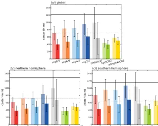
Figure 5. CMIP5 multi-model mean depth and standard deviation (in m) where the individual model mean (left bar) and median (right bar)

depth of thSLR originates for the four RCP scenarios, as well as the historical scenario and the two idealized CO2-forcing scenarios. Thermal

expansion estimates are derived from Eq. (2) based on (a) globally, (b) northern and (c) southern hemispherically averaged vertical potential temperature profiles, followed by a temporal averaging over the last 20 years (see Figs. 3 and 4). Table S5 summarizes the estimates. The horizontal solid (dashed) line indicates the mean (median) depth of thSLR based on climatological temperature and salinity profiles (Boyer et al., 2013).

down to 700 m (cf. Domingues et al., 2008). Sparse obser-vational evidence points to non-significant contributions to global mean thSLR from depths below 2000 m during 2005 to 2013 (Llovel et al., 2014). Our results suggest that 21st century thSLR estimates derived solely based on observa-tional estimates from the upper 700 m would have to be mul-tiplied by a factor of 1.39 (with a 90 % uncertainty range of 1.24 to 1.58) in order to be used as approximation for to-tal thSLR originating from the entire water column. Corre-spondingly, our CMIP5 model analysis suggests that partial thSLR contribution based on hydrographic measurements from the upper 2000 m can be expected to account already for around 85 % of the total thSLR and consequently have to be multiplied only by 1.17 (with a 90 % uncertainty range of 1.05 to 1.31). In fact, our results indicate that half (50 %) of the thSLR contributions can come from depths below 570 m in the historical simulations and from slightly shallower lev-els (490±90 m) in the future RCP scenarios, when averaged across the last 20 years of the scenario period (Fig. 5 and Table S5). Here, we define “half-depth” as the median of the depths distribution of OHU and thSLR contributions. We find that those “half-depths” are located within the thermocline. The OHU half-depth is around 100 m deeper than the thSLR half-depth due to nonlinearities in the seawater equation of state (not shown). Furthermore, those half-depths seem to be

(10)

find-ings highlight the importance of the thSLR contribution from deeper ocean layers (e.g., Palmer et al., 2011). Present and projected thSLR is not predominantly (>50 %) attributable to the layers above the depth of 700 m, the depth most ob-servational based estimated are still limited to (Domingues et al., 2008; Ishii and Kimoto, 2009; Levitus et al., 2012).

Lastly, in order to support the development of surrogate methods to project thermal expansion, we calibrate two sim-plified parameterizations against CMIP5 estimates of thSLR: one parameterization is suitable for scenarios where hemi-spheric ocean temperature profiles are available (1.5-D ap-proach), the other, where only the total OHU (0-D approach) is known. Generally, expanding a mass of warm, salty sub-tropical water is more efficient for a given temperature in-crease than a mass of cold, fresh subpolar water for the same temperature increase. In upper tropical waters a warming sig-nal persists longer than in upper high-latitude waters due to the weaker, temperature-dominated stratification in higher latitudes, except in the Southern Ocean around Antarctica where salinity changes play a fundamental role in determin-ing the strength of stratification (Bindoff and Hobbs, 2013; Rye et al., 2014). Our diagnosis of CMIP5 profiles confirms the large variations inα, the 3-D thermal expansion coeffi-cient, due to strong meridional (not shown) and vertical den-sity gradients originating from strong temperature gradients (see Eq. 2 and Fig 2). These strong vertical as well as merid-ional gradients in the thermal expansion efficiency raise the question whether simplified approaches that collapse either the meridional component (our 1.5-D simplification) or both dimensions (the 0-D approach) are sufficiently reliable. The introduced errors of±5 % (1.5-D) and±9 % (0-D) compared to the CMIP5 data based on the entire ocean grid, suggest that the simplifications are sufficiently accurate for long-term SLR projections, when other uncertainties (land ice-sheet re-sponse, climate sensitivity or radiative forcing (e.g., Hallberg et al., 2013) dominate the final result.

The Supplement related to this article is available online at doi:10.5194/gmd-8-2723-2015-supplement.

Author contributions. All authors contributed to designing and writing the text. K. Lorbacher conducted the analysis and drafted the manuscript.

Acknowledgements. We thank Dimitri Lafleur for his valuable and helpful comments on the manuscript. We acknowledge the World Climate Research Programme’s Working Group on Coupled Mod-elling, which is responsible for CMIP, and we thank the climate modelling groups (listed in Table S1 of this paper and based on http: //cmip-pcmdi.llnl.gov/cmip5/docs/CMIP5_modeling_groups.pdf) for producing and making available their model output. For CMIP

the US Department of Energy’s Program for Climate Model Diagnosis and Intercomparison provides coordinating support and led development of software infrastructure in partnership with the Global Organization for Earth System Science Portals. Observational data by Domingues et al. (2008), Ishii and Kimoto (2009), Levitus et al. (2012) and Roemmich and Gilson (2009) are provided at http://www.cmar.csiro.au/sealevel/sl_data_cmar.html, https://atm-phys.nies.go.jp/~ism/pub/ProjD, http://www.nodc. noaa.gov/OC5/3M_HEAT_CONTENT/basin_tsl_data.html and http://sio-argo.ucsd.edu/RG_Climatology.html, respectively.

Edited by: R. Marsh

References

Abraham, J. P., Baringer, M., Bindoff, N. L., Boyer, T., Cheng, L. J., Church, J. A., Conroy, J. L., Domingues, C. M., Fasullo, J. T., Gilson, J., Goni, G., Good, S. A., Gorman, J. M., Gouret-ski, V., Ishii, M., Johnson, G. C., Kizu, S., Lyman, J. M., Mac-donald, A. M., Minkowycz, W. J., Moffitt, S. E., Palmer, M. D., Piloa, A. R., Reseghetti, F., Schuckmann, K., Trenberth, K. E., Velicogna, I., and Willis, J. K.: A Review of Global Ocean Temperature Observations: Implications for Ocean Heat Con-tent Estimates and Climate Change, Rev. Geophys., 51, 450–483, doi:10.1002/rog.20022, 2013.

Bindoff, N. L. and Hobbs, W. R.: Oceanography: Deep ocean freshening, Nature Climate Change, 3, 864-865, doi:10.1038/nclimate2014, 2013.

Boyer, T. P., Antonov, J. I., Baranova, O. K., Coleman, C., Gar-cia, H. E., Grodsky, A., Johnson, D. R., Locarnini, R. A., Mis-honov, A. V., O’Brien, T. D., Paver, C. R., Reagan, J. R., Seidov, D., Smolyar, I. V., and Zweng, M. M.: World Ocean Database 2013, NOAA Atlas NESDIS 72, edited by: Levitus, S., Technical Editor: Mishonov, A., Silver Spring, MD, 209 pp., doi:10.7289/V5NZ85MT, 2013.

Church, J. A., Clark, P. U., Cazenave, A., Gregory, J. M., Jevrejeva, S., Levermann, A., Merrifield, M. A., Milne, G. A., Nerem, R. S., Nunn, P. D., Payne, A. J., Pfeffer, W. T., Stammer, D., and Un-nikrishnan, A. S.: Sea Level Change, in: Climate Change 2013: The Physical Science Basis. Contribution of Working Group I to the Fifth Assessment Report of the Intergovernmental Panel on Climate Change, edited by: Stocker, T. F., Qin, D., Plattner, G.-K., Tignor, M., Allen, S. G.-K., Boschung, J., Nauels, A., Xia, Y., Bex, V., and Midgley, P. M., Cambridge University Press, Cam-bridge, United Kingdom and New York, NY, USA, 1137–1216, 2013a.

Church, J. A., Monselesan, D., Gregory, J. M., and Marzeion, B.: Evaluating the ability of process based models to project sea-level change, Environ. Res. Lett., 8, 014051, doi:10.1088/1748-9326/8/1/014051, 2013b.

Domingues, C. M., Church, J. A., White, N. J., Gleckler, P. J., Wi-jffels, S. E., Barker, P. M., and Dunn, J. R.: Improved estimates of upper-ocean warming and multi-decadal sea level rise, Nature, 453, 1090–1093, doi:10.1038/nature07080, 2008.

(11)

Durack, P. J., Gleckler, P. J., Landerer, F. W., and Taylor, K. E.: Quantifying underestimates of long-term upper-ocean warming, Nature Climate Change, 4, 999–1005, doi:10.1038/nclimate2389, 2014b.

Forster, P. M., Andrews, T., Good, P., Gregory, J. M., Jackson, L. S., and Zelinka, M.: Evaluating adjusted forcing and model spread for historical and future scenarios in the CMIP5 gener-ation of climate models, J. Geophys. Res.-Atmos., 118, 1139– 1150, doi:10.1002/jgrd.50174, 2013.

Fyfe, J. C., Gillett, N. P., and Thompson, D. W. J.: Compar-ing variability and trends in observed and modelled global-mean surface temperature, Geophys. Res. Lett., 37, L16802, doi:10.1029/2010GL044255, 2010.

Gill, A. E.: Atmosphere-Ocean Dynamics, Acadamic Press, San Diego, California, USA, 662 pp., 1982.

Greatbatch, R. J.: A note on the representation of steric sea level in models that conserve volume rather than mass, J. Geophys. Res., 99, 12767–12771, 1994.

Gregory, J. M., White, N. J., Church, J. A., Bierkens, M. F. P., Box, J. E., van den Broeke, M. R., Cogley, J. G., Fettweis, X., Hanna, E., Huybrechts, P., Konikow, L. F., Leclercq, P. W., Marzeion, B., Oerlemans, J., Tamisiea, M. E., Wada, Y., Wake, L. M., and van de Wal, R. S. W.: Twentieth-century global-mean sea level rise: is the whole greater than the sum of the parts?, J. Climate, 26, 4476–4499, doi:10.1175/JCLI-D-12-00319.1, 2013a.

Gregory, J. M., Bi, D., Collier, M. A., Dix, M. R., Hirst, A. C., Hu, A., Huber, M., Knutti, R., Marsland, S. J., Meinshausen, M., Rashid, H. A., Rotstayn, L. D., Schurer, A., and Church, J. A.: Climate models without volcanic preindustrial volcanic forcing underestimate historical ocean thermal expansion, Geophys. Res. Lett., 40, 1600–1604, doi:10.1002/grl.50339, 2013b.

Griffies, S. M., Yin, J., Durack, P. J., Goddard, P., Bates, S. C., Behrens, E., Bentsen, M., Bi, D., Biastoch, A., Böning, C. W., Bozec, A., Chassignet, E., Danabasoglu, G., Danilov, S., Domingues, C., Drange, H., Farneti, R., Fernandez, E., Greatbatch, R. J., Holland, D. M., Ilicak, M., Large, W., Lor-bacher, K., Lu, J., Marsland, S. J., Mishra, A., Nurser, A. J. G., Salas y Miélia, D., Palter, J. B., Samuels, B. L., Schröter, J., Schwarzkopf, F. U., Sidorenko, D., Treguier, A.-M., Tseng, Y., Tsujino, H., Uotila, P., Valcke, S., Voldoire, A., Wang, Q., Winton, M., and Zhang, X.: An assessment of global and regional sea level for years 1993–2007 in a suite of in-terannual CORE-II simulations, Ocean Modell., 78, 35–89, doi:10.1016/j.ocemod.2014.03.004, 2014.

Hallberg, R., Adcroft, A., Dunne, J. P., Krasting, J. P., and Stouffer, R. J.: Sensitivity of Twenty-First-Century Global-Mean Steric Sea Level Rise to Ocean Model Formulation, J. Climate, 26, 2947–2956, doi:10.1175/JCLI-D-12-00506.1, 2013.

Ishii, M. and Kimoto, M.: Reevaluation of Historical Ocean Heat Content Variations With An XBT depth bias Correction, J. Oceanogr., 65, 287299, doi:10.1007/s10872-009-0027-7, 2009. Jackett, D. R., McDougall, T. J., Feistel, R., Wright, D. G.,

and Griffies, S. M.: Algorithms for density, potential tem-perature, conservative temtem-perature, and the freezing tempera-ture of seawater, J. Atmos. Ocean. Technol., 23, 1709–1728, doi:10.1175/JTECH1946.1, 2006.

Joughin, I., Smith, B. E., and Medley, B.: Marine Ice Sheet Col-lapse Potentially Under Way from the Thwaites Glacier Basin, Science, 344, 735–738, doi:10.1126/science.1249055, 2014.

Kouketsu, S., Doi, T., Kawano, T., Masuda, S., Sugiura, N., Sasaki, Y., Toyoda, T., Igarashi, H., Kawai, Y., Katsumata, K., Uchida, H., Fukasawa, M., and Awaji, T.: Deep ocean heat content changes estimated from observations and reanalysis product and their influence on sea level change, J. Geophys. Res., 116, C03012, dio:10.1029/2010JC006464, 2011.

Kuhlbrodt, T. and Gregory, J. M.: Ocean heat uptake and its conse-quences for the magnitude of sea level rise and climate change, Geophys. Res. Lett., 39, L18608, doi:10.1029/2012GL052952, 2012.

Levitus, S., Antonov, J. I., Boyer, T. P., Baranova, O. K., Garcia, H. E., Locarnini, R. A., Mishonov, A. V., Reagan, J. R., Seidov, D., Yarosh, E. S., and Zweng, M. M.: World ocean heat content and thermosteric sea level change (0–2000 m), 1955–2010, Geophys. Res. Lett., 39, L10603, doi:10.1029/2012GL051106, 2012. Llovel, W., Willis, J. K., Landerer, F W., and Fukumori, I.:

Deep-ocean contribution to sea level and energy budget not detectable over the pa st decade, Nature Climate Change, 4, 1031–1035, doi:10.1038/nclimate2387, 2014.

Lorbacher, K., Marsland, S. J., Church, J. A., Griffies, S. M., and Stammer, D.: Rapid barotropic sea level rise from ice sheet melt-ing, J. Geophys. Res., 117, C06003, doi:10.1029/2011JC007733, 2012.

Lowe, J. A. and Gregory, J. M.: Understanding projections of sea level rise in a Hadley Centre coupled climate model, J. Geophys. Res., 111, C11014, doi:10.1029/2005JC003421, 2006.

Meinshausen, M., Raper, S. C. B., and Wigley, T. M. L.: Emulat-ing coupled atmosphere-ocean and carbon cycle models with a simpler model, MAGICC6 – Part 1: Model description and cal-ibration, Atmos. Chem. Phys., 11, 1417–1456, doi:10.5194/acp-11-1417-2011, 2011.

Mengel, M. and Levermann, A.: Ice plug prevents irreversible dis-charge from East Antarctica, Nature Climate Change, 4, 451– 455, doi:10.1038/nclimate2226, 2014.

Moss, R. H., Edmonds, J. A., Hibbard, K. A., Manning, M. R., Rose, S. K., van Vuuren, D. P., Carter, T. R., Emori, S., Kainuma, M., Kram, T., Meehl, G. A., Mitchell, J. F., Nakicenovic, N., Ri-ahi, K., Smith, S. J., Stouffer, R. J., Thomson, A. W., Weyant, J. P., and Wilbanks, T. J.: The next generation of scenarios for climate change research and assessment, Nature, 463, 747–756, doi:10.1038/nature08823, 2010.

Palmer, M. D., Good, S. A., Haines, K., Rayner, N. A., and Stott, P. A.: A new perspective on warming of the global oceans, Geo-phys. Res. Lett., 36, L20709, doi:10.1029/2009GL039491, 2009. Palmer, M. D., McNeall, D. J., and Dunstone, N. J.: Impor-tance of the deep ocean for estimating decadal changes in Earth’s radiation balance, Geophys. Res. Lett., 38, L13707, doi:10.1029/2011GL047835, 2011.

Palter, J. B., Griffies, S. M., Samuels, B. L., Galbraith, E. D., Gnanadesikan, A., and Klocker, A.: The Deep Ocean Bouyancy Budget and Its Temporal Variability, J. Climate, 27, 551–573, doi:10.1175/JCLI-D-13-00016.1, 2014.

Piecuch, C. G. and Ponte, R. M.: Mechanisms of Global-Mean Steric Sea Level Change, J. Climate, 27, 824–834, doi:10.1175/JCLI-D-13-00373.1, 2014.

(12)

Raper, S. C. B., Wigley, T. M. L., and Warrick, R. A.: Global Sea-level Rise: Past and Future, in: Sea-Level Rise and Coastal Sub-sidence: Causes, Consequences and Strategies, edited by: Milli-man, J. and Haq, B., Kluwer, Dordrecht, the Netherlands, 11–45, 1996.

Rhein, M., Rintoul, S. R., Aoki, S., Campos, E., Chambers, D., Feely, R. A., Gulev, S., Johnson, G. C., Josey, S. A., Kostianoy, A., Mauritzen, C., Roemmich, D., Talley, L. D., and Wang, F.: Observations: Ocean, in: Climate Change 2013: The Physical Science Basis. Contribution of Working Group I to the Fifth Assessment Report of the Intergovernmental Panel on Climate Change, edited by: Stocker, T. F., Qin, D., Plattner, G.-K., Tig-nor, M., Allen, S. K., Boschung, J., Nauels, A., Xia, Y., Bex, V., and Midgley, P. M., Cambridge University Press, Cambridge, United Kingdom and New York, NY, USA, 2013.

Rignot, E., Mouginot, J., Morligem, M., Serossi, H., and Scheuchl, B.: Widespread, rapid grounding line retreat of Pine Is-land, Thwaites, Smith and Kohler glaciers, West Antarctica from 1992 to 2011, Geophys. Res. Lett., 41, 3502–3509, doi:10.1002/2014GL060140, 2014.

Roemmich, D. and Gilson, J.: The 2004–2008 mean and annual cycle of temperature, salinity, and steric height in the global ocean from the Argo Program, Prog. Oceanogr., 82, 81–100, doi:10.1029/2011GL047992, 2009.

Rose, B. E. J., Armour, K. C., Battisti, D. S., Feldl, N., and Knoll, D. D. B.: The dependence of transient climate sensitivity and radia-tive feedbacks on the spatial pattern of ocean heat uptake, Geo-phys. Res. Lett., 41, 1071–1078, doi:10.1002/2013GL058955, 2014.

Russell, G. L., Gornitz, V., and Miller, J. R.: Regional sea level changes projected byb the NASA/GISS Atmosphere Ocean Model, Clim. Dynam., 16, 789–797, 2000.

Rye, C. D., Naveira Garabato, A. C., Holland, P. R., Mered-ith, M. P., Nurser, A. J., Hughes, C. W., Coward, A. C., and Webb, D.: Rapid sea-level rise along the Antarctic margins in re-sponse to increased glacial discharge, Nat. Geosci., 7, 732–735, doi:10.1038/ngeo2230, 2014.

Sen Gupta, A., Jourdain, N. C., Brown, J. N., and Monselesan, D.: Climate Drift in the CMIP5 Models, J. Climate, 26, 8597–8615, doi:10.1175/JCLI-D-12-00521.s1, 2013.

Taylor, K. E., Stouffer, R. J., and Meehl, G. A.: An Overview of CMIP5 and the scenario design, B. Am. Meteorol. Soc., 93, 485– 498, doi:10.1175/BAMS-D-11-00094.1, 2012.

Trenberth, K. E. and Fasullo, J. T.: Tracking Earth’s Energy, Sci-ence, 238, 316–317, doi:10.1126/science.1187272, 2010. Wang, C., Zhang, L., Lee, S.-K., Wu, L., and Mechoso, C. R.: A

global perspective on CMIP5 climate model biases, Nature Cli-mate Change, 4, 201–205, doi:10.1038/ncliCli-mate2118, 2014. Wigley, T. M. L., Clarke, L. E., Edmonds, J. A., Jacoby, H. D.,

Palt-sev, S., Pitcher, H., Reilly, J. M., Richels, R., Sarofim, M. C., and Smith, S. J.: Uncertainties in climate stabilization, Climatic Change, 97, 85–121, doi:10.1007/s10584-009-9585-3, 2009. Yin, J.: Century to multi-century sea level rise projections