Multilayered Structures under large Bending: Finite Solution and Bifurcation Analysis

University of Trento

Sara Roccabianca

MULTILAYERED STRUCTURES UNDER

LARGE BENDING: FINITE SOLUTION AND

BIFURCATION ANALYSIS

Engineering of Civil and Mechanical Structural Systems, Cycle XXIII

Ph.D. program Head: Davide Bigoni

Final Examination: 25/03/2011

Board of Examiners

Prof. Roberto Oboe (Universit`a degli Studi di Padova) Prof. Robert McMeeking (University of California) Prof. Ettore Pennestri (Universit`a degli Studi di Roma)

Abstract

Contents

1 Introduction 7

2 Notation and governing equations 15

3 Finite bending of a layered block 19

3.1 Kinematics . . . 19

3.2 Stress . . . 23

3.3 Examples of multilayered plates under finite bending . . . 25

4 In-plane incremental bifurcations 29 4.1 General formulation . . . 29

4.2 Bifurcation of a bilayer . . . 34

5 Numerical procedures 47 5.1 The determinantal method . . . 47

5.2 The compound matrix method for a bilayer . . . 50

6 Experiments on rubber blocks 57 7 Out-of-plane incremental bifurcations 67 7.1 General formulation . . . 67

7.2 Examples . . . 74

7.2.1 The homogeneous block . . . 74

8 Conclusions 83

A Matrices of numerical methods 85

1

Introduction

Figure 1.1: Left: a stiff (30 mm thick, neoprene) layer bonded by two com-pliant (100 mm thick foam) layers in a rigid wall and confined compression ap-paratus (note that a separation between sample and wall has occurred on the right upper edge of the sample). Centre: creases occurring at the compressive side of a rubber strip, coated at the tensile side with a 0.4 mm thick polyester transparent film, subject to flexure. Right: bifurcation of a two-layer rubber block under finite bending evidencing long-wavelength bifurcation modes (the stiff layer, made up of natural rubber, is at the compressive side of a neoprene block).

tension or compression, Refs. [30,35,57].

In this thesis we have generalized the solution for plane strain bending of an elastic block given by Rivlin, Ref. [42], and the subsequent analyses of incremental bifurcations, Refs. [1, 2, 12, 13,17, 22, 52], determinating the stress/strain fields during finite bending for elastic multilayers and related bifurcation analysis.

Finite bending of plates is a phenomenon common in nature and in engineered processes. Leaves are often subject to large bending for var-ious reasons: the pinguicola leptoceras, curls its leaf to trap insects, the

geranium–pratensis’ pod suffers a strong bending when seeds are dispersed,

andgramineae leaves deform into a tube to resist dehydratation. Moreover,

tissue-engineered blood vessels, in which the internal fibroblast sheets arewrapped

around a tubular support, Ref. [31]. In microelectronic devices, we may mention that flexible solar cells (made up of layers, one of which contain-ing three-dimensional nanopillar-array photovoltaics) have a 4 mm thickness and are subject to bending up to a curvature radius of 3 cm, Ref. [23].

Althoughplates suffering finite bending are often made up of layers1, the theory of finite elastic bending has been previously developed only under the assumption of homogeneity, Ref. [27, 34, 42, 55]. Moreover, while certain elastic multilayers can be bent until the tubular shape is reached without any appearance of inhomogeneities, crazes develop for other systems (Fig. 1.1, in the centre, and also Fig. 6.5), severely decreasing the elastic deformational capability.

Since these crazes can be interpreted as bifurcation modes localized near the surface, the bifurcation analysis becomes an important tool for design purposes. However, theoretical, Ref. [12,13,17,22,28,52], and experimen-tal, Ref. [26], approaches to bifurcation of plates subject to finite bending have only been considered until now under the assumption of material ho-mogeneity. Therefore, the aims of the present thesis are:

(i.) to provide an analytical solution to finite bending of an elastic multi-layered thick plate deformed under the plane strain constraint; (ii.) to analyse and solve the problem of two-dimensional bifurcations

pos-sibly occurring during bending;

(iii.) to validate our theoretical approach with experiments.

Analyzing the incremental problem we found that for several geometries and stiffness contrasts the first (‘critical’) bifurcation load corresponds to a long-wavelength mode, which results to be very close to the bifurcation

1_{Leaves, arteries, and the flexible solar cells, Ref. [23], are complex structures}

load associated with the surface instability limit of vanishing wavelength2, a feature also common to the behaviour of a homogeneous elastic block subject to finite bending. This feature explains the experimental observation (on uniform blocks, Ref. [25,26]) that short-wavelength modes become visible, instead of the long-wavelength modes that are predicted to occur before. Therefore, the question was left open whether or not wavelength modes longer than the short-wavelength modes available at surface instability and visible in the experiments can be experimentally displayed with a layered system in which an appropriate selection is made of stiffness and thickness contrast between layers. We provide a positive answer to this problem in this thesis, so that our calculations, based now on the compound matrix method, Ref. [4, 36–38], allow us to conclude that there are situations in which the long-wavelength modes are well-separated from the surface instability, so that systems exhibiting bifurcation modes of long wavelength can be designed. These systems have been realized by us and qualitatively tested, showing that the theory predictions are generally followed, Fig. 1.1

on the right.

The solution for finite bending of an elastic multilayer discloses the com-plex stress distributions that can be generated inside such structures as a result of large strains. For instance, more than one neutral axis may be present3 _{(Fig. 3.3) and weakly stressed layers may ‘bond’ a highly stressed}

one (Fig. 3.4). The determination of these stress states is of great impor-tance in the design of multilayered structures, but then the question arises

2 _{Surface instability occurs in a uniformly strained half space as a bifurcated mode}

of arbitrary wavelength, corresponding to a Rayleigh wave of vanishing speed. In the limit of vanishing wavelength, surface instability can be viewed as a bifurcation mode ‘adaptable’ to every boundary and state of stress of a strained body, so that it becomes a local instability mode (also called ‘failure of complementing condition’, Ref. [5]).

3 _{In our examples we have found situations with two (Fig. 3.2) and three (Fig. 3.3)}

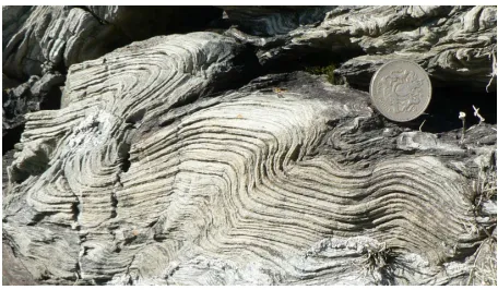
Figure 1.2: Bifurcation in compression of a finely layered metamorphic rock has induced severe folding, an example of a ‘accomodation structure’ (Treard-dur Bay, Holyhead, N. Wales, UK; the coin in the photos is a Pound).

if such configurations can be achieved without encountering a previous bi-furcation. In fact, one conclusion of the bifurcation analysis is that there is a strong difference between bifurcation loads and geometries when homo-geneous structures are compared with the corresponding layered structures. For instance, a stiff and thin coating reinforcing an elastic layer strongly decreases the bifurcation bending angle of the uncoated structure, a find-ing fully consistent with the solutions obtained employfind-ing a surface coatfind-ing model by Dryburgh and Ogden and Gei and Ogden, Ref. [22, 24]. In a bilayer, two neutral axes typically occur when a stiff layer is placed at the compressive side of the system, a case in which the differential equations be-come ‘numerically stiff’, so that we have employed an ‘ad hoc version’ of the compound matrix method, which is shown to allow systematic investigation of the situations in which more than one neutral axis occurs. In these cases we find a sort of ‘inversion’ of the sequence of bifurcation modes with the aspect ratio of the system, so that high-wavenumber modes are relevant for lower slender ratios than small-wavenumber modes.

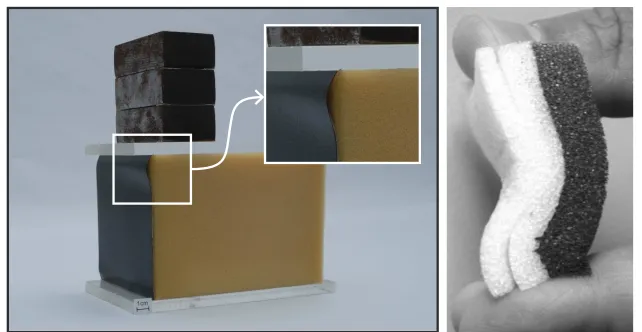
Figure 1.3: Bifurcation in compression with detachment of layers: a stiff (1 mm thick) plastic coating is detached from a foam substrate to which it was initially glued (left), three layers of foam fold with detachment, clearly visible near the edges of the sample (right).

bending have been investigated only by Gent and Cho, Ref. [26], although the experimental setting is not particularly complex. To extend their analy-ses to the case of layered plates, we have designed a simple device to impose a bending angle to elastic strips on which bifurcations in the form of crazes can be detected by direct visual inspection.

The bifurcation loads and modes are strongly sensible to the bonding conditions between the layers, which may be perfect (as in the case of the rock shown in Fig. 1.2), but often they are may involve the possibility of slip and detachments, the so-called ‘delaminations’ (as in the cases shown in Figs. 1.3).

displace-ments, that are unrestricted. For simplicity, the materials forming the mul-tilayer are assumed hyperelastic and incompressible, according to the gen-eral framework laid by Biot, Ref. [11], in which Mooney-Rivlin and Ogden materials, Ref. [39], as well as the J2–deformation theory of plasticity, are

2

Notation and governing

equations

The notation employed throughout the present thesis and the main equa-tions governing equilibrium in finite and incremental elasticity are now briefly recalled. Let x0 denote the position of a material point in some stress-free reference configuration B0 of an elastic body. A deformation ξ

is applied, mapping points of B0 to those of the current configuration B

indicated by x = ξ(x0). We identify its deformation gradient by F, i.e., F = Gradξ, and we define the right, C, and the left, B, Cauchy-Green tensors as C =FTF and B =F FT.

For isotropic incompressible elasticity the constitutive equations can be written as a relationship between the Cauchy stress T and B as

T =−πI+α1B+α−1B−1, detB = 1, (2.1)

where π is an arbitrary Lagrangian multiplier representing a hydrostatic pressure andα1, α−1 are coefficients which may depend on the deformation.

(i = 1,2,3). In the case of an incompressible material these relationships take the form (indexinot summed)

Ti =−π+λi

∂W(λ1, λ2, λ3)

∂λi

, λ1λ2λ3 = 1, (2.2)

Eqs. (2.1) and (2.2) are linked through the following equations (Ref. [7]) α1=

1 λ2

1−λ22

(T1−T3)λ21

λ2 1−λ23

−(T2−T3)λ

2 2

λ2 2−λ23

,

α−1=

1 λ2

1−λ22

T1−T3

λ2 1−λ23

−T2−T3 λ2

2−λ23

,

(2.3)

that allow to express coefficients α1, α−1 in terms of the strain energy of

the body.

In the absence of body forces, equilibrium is expressed in terms of the first Piola-Kirchhoff stress tensor S =JT F−T as DivS =0, where Div is the divergence operator defined inB0.

Loss of uniqueness of the plane-strain incremental boundary-value prob-lem is investigated, so that incremental displacements are given by

u(x) = ˙ξ(x0), (2.4) where, henceforth, a superposed dot is used to denote a first-order increment. The incremental counterpart of equilibrium is expressed bydivΣ=0, where

divis the divergence in the current configuration. The updated incremental first Piola-Kirchhoff stress is given by

Σ= ˙S FT, S˙ = ˙T F−T −T LTF−T. (2.5) The linearized constitutive equation is

Σ=C_{L−πI˙ , (2.6)}

whereL = gradu and C _{is the fourth-order tensor of instantaneous elastic}

trL= 0. Since Σ= ˙T −T LT, the balance of rotational momentum yields Σ12−Σ21=T2L12−T1L21, and a comparison with eq. (2.6) shows that (no

sum on indices i andj)

Cijji+Ti =Cjiji (i6=j). (2.7) For a hyperelastic material, the components ofC_{can be defined in terms of}

the strain-energy function W.

For the plane strain problem addressed here the fourth-order tensor C

can be written in terms of 2 incremental moduli µ and µ∗_{, their explicit} form will be given

µ= λ 2

λ4+ 1 λ4₋₁

dWˆ dλ

!

, µ∗= λ 4

dWˆ dλ +λ

d2Wˆ dλ2

!

, (2.8)

where ˆW =W(λ,1/λ,1), due to incompressibility. In the following, exam-ples are given for a neo-Hookean material, which is the initially isotropic elastic solid with strain energy given by

W = µ0 2 λ

2

1+λ22−2

, (2.9)

whereλ1and λ2 are the principal in-plane stretches. Due to

incompressibil-ity λ=λ1 and λ2= 1/λ, so that

T1 =µ0(λ2−λ−2), and µ=µ∗=

µ0

2 (λ

2_+λ−2_{), (2.10)}

where the former is the uniaxial tension law (along axisx2). Notice that the

ratio between T1 and µis

T1

µ =

2(λ2−λ−2₎

λ2_+λ−2 , (2.11)

In the case of an out-of-plane analysis the fourth-order tensor C _is

de-pendent on six moduliµi and µ∗i (i= 1,2,3) (no sum on index), see Refs. [11,39], which for a hyperelastic material can be written as

2µ∗_i =λi ∂W ∂λi

+λ2_i∂

2_W

∂λ2

i

−X l6=i

λiλl ∂2W ∂λi∂λl

+λjλk ∂2W ∂λj∂λk

(j6=k6=i),

2µi = (Tj−Tk)

λ2_j+λ2_k

λ2_j−λ2_k (j6=k6=i).

(2.12) In the ensuing analysis of multilayers two types of interface conditions will be employed: perfect bonding, where both incremental tractions and displacements are continuous and imperfect interface (compliant interface), where the incremental shear stress is linearly dependent on the jump of incremental transverse displacement.

In the former case, where the layers are perfectly bonded, the imposed interfacial conditions are:

• continuity of tractions across the interface

Σ+n =Σ−n; (2.13)

• continuity of incremental displacements

u+=u−. (2.14)

In the latter case, we employ a particular case of the compliant interface model of Suo et al. and Bigoni et al. (Ref. [51] and [9]) for which, in addition to eqn. (2.13), the radial incremental displacement ur is continuous across the interface while a compliant law relating the incremental shear stress to the transverse displacement jump is imposed, namely

Σ(_θrs)

r=r(es)

=S_θu(s+1)+

θ −u

(s)−

θ

. (2.15)

3

Finite pure bending of an

elastic layered block

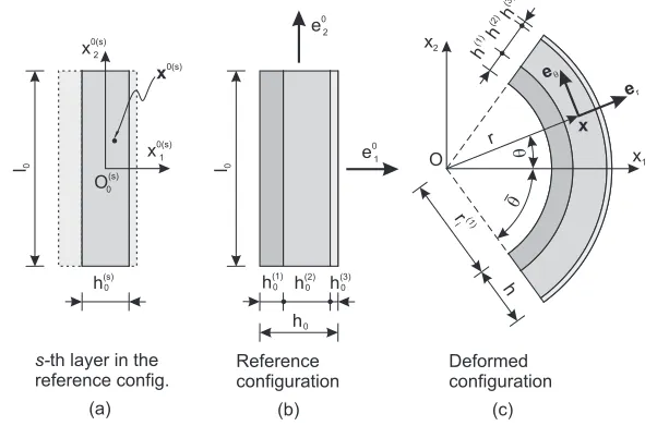
The solution for pure bending of an elastic layered thick plate made up ofN layers follows from ‘assembling’ solutions relative to the bending of all layers taken separately, a solution first given by Rivlin (Ref. [42]). Therefore, we begin recalling this solution with reference now to a generic layer. To this purpose, we consider plane-strain flexure of an incompressible rectangular elastic layered plate, of initial dimensions l0×h0 (see Fig. 3.1b).

3.1

Kinematics

In the reference stress-free configuration, a Cartesian coordinate system O₀(s)x0(₁s)x₂0(s)x0(₃s) is introduced for each layer denoted by index s, centered at its centroid (see Fig. 3.1a). Denoting by e0_i (i = 1,2,3) the common cartesian basis, the position of the generic point x0(s) is given by

x0(s)=x0(₁s)e0₁+x₂0(s)e0₂+x0(₃s)e0₃, (3.1) with

h (1) h(3) 0 l0 q q er r eq x1 e0 1

x2 h

(2) h (3) r i (1) h e0 2 h(2) 0 h(1) 0 h0 Reference configuration Deformed configuration x x0(s) 1 x0(s) 2 x0(s) O(s) 0 (b) (c) (a) s-th layer in the reference config.

h(s) 0

O

l0

Figure 3.1: Sketch of a generic layered thick plate subject to finite bending.

The deformed configuration is a portion of a cylindrical tube of semi-angle ¯θ. It is useful to introduce here a cylindrical coordinate system O(s)_r(s)_θ(s)_z(s)_{, with basis e}

r, eθ and ez, where points of the s−th layer are transformed to points identified by

r(s)∈[r(_is), r(_is)+h(s)], θ(s)∈[−θ,¯ +¯θ], z(s)∈(−∞,+∞). The deformation is prescribed in a way that a plane at constant x0(₁s) transforms to a circular arc at constantr(s)_{, while a plane at constant x}0(s)

2

transforms to a plane at constantθ(s). The out-of-plane deformation is null, so thatx0(₃s)=z(s). The incompressibility constraint (conservation of areas) imposes that

r_i(s)= l0h

(s) 0

2¯θh(s) −

h(s)

2 , (3.3)

whereh(s) _{is the current thickness of the circular sector, to be determined.}

The deformation, in this condition, is described by functions

3.1 Kinematics

so that the deformation gradient takes the form F(s)= dr

(s)

dx0(₁s)er⊗e

0 1+r(s)

dθ(s)

dx0(₂s)eθ⊗e

0

2+ez⊗e03. (3.5)

The right and left Cauchy-Green tensors are

C(s)= dr

(s)

dx0(₁s)

!2

e0₁⊗e0₁+ r(s) dθ

(s)

dx0(₂s)

!2

e0₂⊗e0₂+e0₃⊗e0₃,

B(s)= dr

(s)

dx0(₁s)

!2

er⊗er+ r(s) dθ(s)

dx0(₂ s)

!2

eθ⊗eθ+ez⊗ez,

(3.6)

so that we identify the principal stretches to be λ(_rs)= dr

(s)

dx0(₁ s), λ

(s)

θ =r( s) dθ(s)

dx0(₂s), and λ

(s)

z = 1. (3.7) Imposition of the incompressibility constraint reduces the deformation to the simple form

r(s)=

r

2 α(s)x

0(s)

1 +β(s), θ(s) =α(s)x

0(s)

2 , (3.8)

so that, using eqn. (3.4), the principal stretches can be evaluated as λ(_rs)= 1

α(s)_r(s), λ (s)

θ =α(

s)_r(s)_{, and λ}(s)

z = 1, (3.9) where α(s) _{and β}(s) _{are constants which are fixed by boundary conditions.}

For the s–th layer of a multilaminated, these are

• at x0(₂s) = ±l0/2, θ(s) = ±θ¯, from eqn. (3.8)2, θ(s) = ±α(s)l0/2,

yielding

α(s)= 2¯θ l0

; (3.10)

note that α(s) is independent of the index s;

• at x0(₁ s) = −h(₀s)/2, r(s) = r(_is), from eqns. (3.3) and (3.8)1, ri(s) = r(s)_(−h(s)

0 /2), yielding

β(s)=r_i(s)2 +l0h

(s) 0

Since theN layers are assumed to be perfectly bonded to each other and thes–th layer has current thicknessh(s)_{, we have}

r_i(s)=r(_is−1)+h(s−1) (s= 2, . . . , N), (3.12)

withr(1)_i given byr_i(1)=l0h0(1)/(2¯θh(1))−h(1)/2, see eqn. (3.3). A repeated

use of eqns. (3.3) and (3.12) provides all thicknesses h(s) _{(s = 2, ..., N)}

expressed in terms of the thickness of the first layerh(1)_{, which remains the}

sole kinematical unknown of the problem, determined from the solution of the boundary-value problem described in Section3.2.

Since eqn. (3.12) is imposed at each of the N −1 interfaces between layers, all radial coordinates r(s) share the same origin O of a new cylin-drical coordinate system Orθz, common to all deformed layers (Fig. 3.1c); therefore, index s on the local current coordinates will be omitted in the following so that the deformed configuration will be described in terms of the global systemOrθz.

As a conclusion, the kinematics provides all the stretches in the multi-layered which can be represented as

λr = l0

2¯θr, λθ = 2¯θr

l0

, and λz = 1, (3.13)

and the current thickness of the s–th layer, h(s)_{, as a function of h}(s−1)_,

namely

h(s)=−l0h

(s−1) 0

2¯θh(s−1)−

h(s−1) 2 +

v u u t l0h

(s−1) 0

2¯θh(s−1) +

h(s−1)

2

!2

−l0h

(s) 0

¯

3.2 Stress

3.2

Stress

We are now in a position to determine the stress state within the multilayer. In particular, the Cauchy stress tensor in generic layer scan be written as

T(s)=T_r(s)er⊗er+T( s)

θ eθ⊗eθ+Tz(s)ez⊗ez, (3.15) where, from the constitutive equations (2.2),

T_r(s)=−π(s)+λr ∂W(s)

∂λr

, T_θ(s)=−π(s)+λθ ∂W(s)

∂λθ

, (3.16)

T_z(s)=−π(s)+ ∂W

(s)

∂λz

λz=1

.

Since stretches depend only onr, the chain rule of differentiation d·

dr = ∂· ∂λr

dλr dr +

∂· ∂λθ

dλθ

dr , (3.17)

together with eqns. (3.16) and the derivatives of stretches with respect tor calculated from eqn. (3.9), can be used in the equilibrium equations

∂Tr(s) ∂r +

Tr(s)−T_θ(s) r = 0,

∂T_θ(s)

∂θ = 0, (3.18) to obtain the identities

dW(s)

dr =−

Tr(s)−T_θ(s)

r =

dTr(s)

dr . (3.19)

Therefore, identifyingλθ withλ, we arrive at the expression

Tr(s)(r) = ˆW(s)(λ(r)) +γ(s), (3.20) where

ˆ

W(s)(λ(r)) =W(s)(1/λ(r), λ(r),1), (3.21) and γ(s) _{is an unknown integration constant. From eqn. (3.18)}

1 we finally

obtain

T_θ(s)(r) = 2¯θ l0

where the prime denotes, now, differentiation with respect toλ

Constants γ(s) _{(s = 1, . . . , N) and thickness h}(1) _{can be calculated by}

imposing: (i.) continuity of tractions at interfaces between layers (N −1 equations) and (ii.) traction boundary conditions at the external boundaries of the multilayer (2 equations). ConsideringN layers, the traction continuity at the interfaces write as

Tr(s−1)(r

(s−1)

i +h(s−1)) =Tr(s)(r

(s)

i ) (s= 2, . . . , N), (3.23) while null loading at the external surfaces of the multilayer yields

T_r(1)(r_i(1)) = 0, T_r(N)(r(_iN)+h(N)) = 0. (3.24)

Therefore,γ(N) can be calculated from eqn. (3.24)2

γ(N) =−Wˆ(N)λ(r_i(N)+h(N)), (3.25)

while employing eqn. (3.23), we obtain the recursive formulae

γ(s−1)= ˆW(s)λ(r(_is))−Wˆ(s−1)λ(r_i(s))+γ(s) (s= 2, . . . , N). (3.26)

Considering now eqn. (3.24)1 and evaluating γ(1) from eqn. (3.26)

writ-ten fors= 2, we obtain an implicit expression to be solved forh(1) ˆ

W(2)λ(r_i(2))−Wˆ(1)λ(r_i(2))+ ˆW(1)λ(r_i(1))+γ(2) = 0, (3.27)

where h(2) _{and γ}(2) _{are functions of h}(1)_{, through eqns. (3.14) and (3.26),}

respectively.

3.3 Examples of multilayered plates under finite bending

3.3

Examples of multilayered plates under finite

bending

The solution obtained in the previous section is interesting in itself and can be easily used for design purposes, since it allows determination of the complex stress and strain fields within a thick, multilayered plate, when subject to finite bending. To highlight the usefulness of the solution, we present a few results for finite bending of an elastic thick plate, coated with a thin and stiff layer, and of a three- and five- layer structures, assuming a neo-Hookean behaviour for both materials.

Deformed geometries for the coated layer (withl0/h0= 2,h(0lay)/h (coat)

0 =

10 andµ(coat)/µ(lay) = 20) are shown in Fig. 3.2, together with graphs of the dimensionless Cauchy principal stresses Tr(r)/µ(lay) _{and T}

θ(r)/µ(lay). The deformed configurations plotted in the upper part of Fig. 3.2correspond to critical configurations at bifurcation (see Section 4.2), while those reported in the lower part lie beyond the critical bifurcation threshold, so that they are reported only with the purpose to show the evolution of the solution of finite bending at very large angles. Note that the transverse stress is always compressive, while the distribution of Tθ(r) strongly depends on the stiffness of the layer under consideration and gives a null resultant, so that it is equivalent to the bending moment loading the plate. For all cases, the neutral axis (the line corresponding to vanishing circumferential stress) is drawn, showing the effect of the coating on the global stress state. Note that in the lower figure on the left, two neutral axes are visible. This is an important feature, which is also investigated in Fig. 3.3, referred to a three-layer plate. In this structure, where the initial aspect ratio is 1, the shear stiffness contrast is 20 and ratio between layer thicknesses is 5, three

neutral axes become visible starting from a bending semi-angle of 56◦, so

1

T /rm (lay)

T /qm

(lay)

T /qm

(lay)

T /qm

(lay)

T /qm

(lay)

T /rm (lay)

T /rm (lay)

T /rm (lay)

l /h =2 h /h =10

/ =20

0 0

0 0

(lay) (coat)

(coat) (lay)

m m q=1.13 rad

q=2.44 rad

q=0.65 rad

q=2.44 rad +

-- +

-5

+

+

-neutral axes

T /qm ,T /m

(lay) (lay)

r T /qm , T /m

(lay) (lay)

r

Figure 3.2: Undeformed (center) and deformed (upper and lower parts) shapes and internal stress states for finite bending of neo-Hookean coated plates with l0/h0 = 2, h(lay)0 /h

(coat)

0 = 10 and µ(coat)/µ(lay) = 20. Dashed

3.3 Examples of multilayered plates under finite bending

material (a) material (b) material (c)

T /q m , T /m

(b) (b)

r 1

l /h =1

/ =20

0 0

m m(a) (b)

h /h =5 h /h =5

/ =20

0 0

0 0

(b) (a)

(c) (b)

(b) (c)

m m

neutral axes

T /qm

(b)

T /rm (b)

+

-Figure 3.3: Finite bending of a neo-Hookean three-layer plate showing three neutral axes.

T /qm

(b)

T /rm (b) T /q m , T /m

(b) (b) r

material (a) material (b) T /qm

(b)

T /qm

(b)

T /rm (b)

T /rm (b)

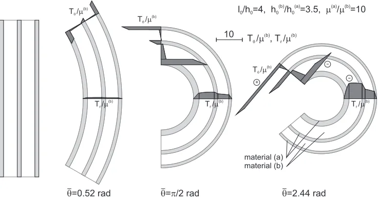
l /h =4, h /h =3.5,0 0 0 0 / =10

(b) (a) (a) (b)

m m

+

-q=0.52 rad q= /2 radp q=2.44 rad 10

Figure 3.4: From left to right: undeformed and progressively more deformed shapes and internal stress states for finite bending of a neo-Hookean five-layer plate with l0/h0 = 4, h(b)0 /h

(a)

0 = 3.5, µ(a)/µ(b) = 10. Note the scales of

l0/h0 = 4 is reported in Fig. 3.4, where three configurations are shown at

different bending angles ¯θ. The layers are made up of two materials, (a) and (b), such that h(₀b)/h(₀a) = 3.5 and µ(a)_/µ(b) _{= 10. As in Fig. 3.2, the two}

4

In-plane incremental

bifurcations superimposed on

finite bending of an elastic

layered block

The goal of this section is to address the plane-strain bifurcation problem of the multilayered thick plate subject to finite bending, considered in Chapter

3.

4.1

General formulation

We begin by analyzing the incremental field equations for an isolated layer and we continue formulating the multilayered problem by adding the relevant interfacial and external boundary conditions. We refer to Chapter2 for the notation.

The gradient of incremental displacement u(x) is

L=ur,rer⊗er+

ur,θ−uθ

r er⊗eθ+uθ,reθ⊗er+

ur+uθ,θ

and the incompressibility condition (trL= 0) can be written in polar coor-dinates as

rur,r+ur+uθ,θ= 0. (4.2) For an incompressible isotropic elastic material, the components of the constitutive fourth-order tensorC_{[see eqn. (2.6)] can be written as function}

of two incremental moduli, denotedµand µ∗, that depend on the deforma-tion. The non-vanishing components ofC_{may be expressed as}

Crrrr=Cθθθθ = 2µ∗+p, Cθrθr =µ−Γ,

Crθrθ =µ+ Γ, Crθθr =Cθrrθ =µ+p,

(4.3)

where

Γ = Tθ−Tr

2 , p=−

Tθ+Tr

2 (4.4)

describe the state of prestress. For hyperelastic materials, µand µ∗ can be given in terms of the strain-energy function ˆW(λ) as

µ= λ 2

λ4+ 1 λ4₋₁

dWˆ dλ

!

, µ∗ = λ 4

dWˆ dλ +λ

d2Wˆ dλ2

!

. (4.5)

The incremental constitutive equations in terms of the incremental first Piola-Kirchhoff stress tensor can be written as

Σrr=−π˙+ (2µ∗+p)ur,r, Σθθ =−π˙+ (2µ∗+p)

ur+uθ,θ

r ,

Σrθ= (µ+ Γ)

ur,θ−uθ

r + (µ+p)uθ,r, Σθr= (µ+p)

ur,θ−uθ

r + (µ−Γ)uθ,r. (4.6) A substitution of eqns. (4.6) and the use of eqn. (3.18)1 in the

incre-mental equations of equilibrium written in polar coordinates Σrr,r+1

rΣrθ,θ+

Σrr−Σθθ r = 0, Σθr,r+1

rΣθθ,θ+

Σθr+ Σrθ r = 0,

4.1 General formulation

yields the incremental equilibrium equations written in terms of incremental displacements and in-plane mean stress

˙ π,r =

(p+ 2µ∗),r+

2(p+ 2µ∗) r

ur,r+ (p+ 2µ∗)ur,rr +(µ+ Γ)ur,θθ−uθ,θ

r2 + (p+µ)

uθ,rθ r ,

˙

π,θ= [r(µ−Γ),r+µ−Γ]

uθ,r+

ur,θ−uθ r

+r(µ−Γ)uθ,rr+ (µ−2µ∗)ur,θr. (4.8) We seek bifurcations in the following separable-variables form

        

ur(r, θ) =f(r) cosnθ, uθ(r, θ) =g(r) sinnθ,

˙

π(r, θ) =k(r) cosnθ,

(4.9)

where f(r), g(r) and k(r) are real functions and n is a real number to be determined by imposing boundary conditions.

Consideration of the incompressibility constraint g=−(f +rf

0₎

n , (4.10)

and substitution of representations (4.9) into eqns. (4.8) yields k0=Df00+

C,r+D,r+

C+ 2D r

f0+E(1−n

2₎

r2 f,

k= r

2_C

n2 f

000₊ F+ 3C n2 rf

00₊

F n2 −D

f0− 1−n

2

n2

F rf,

(4.11)

where a prime denotes differentiation with respect to r and in terms of in-cremental moduliµandµ∗and strain-energy function ˆW(λ), the coefficients C,D,E and F can be expressed as

C =µ−Γ = λ λ4₋₁

dWˆ

dλ , D= 2µ∗−µ= λ 2 λ

d2_Wˆ dλ2 −

2 λ4₋₁

dWˆ dλ

!

,

E =µ+ Γ = λ

5

λ4₋₁

dWˆ

dλ , F =rC,r+C.

By differentiating eqn. (4.11)2 with respect to r and substituting it into

eqn. (4.11)1, a single differential equation in terms of f(r) is obtained

Cr4f0000+ 2(F + 2C)r3f000+ [(rF),r+ 4F−2n2D]r2f00

+[(rF −2rn2D),r−2F]rf0+ (1−n2)(F −rF,r−n2E)f = 0.

(4.13)

Eqn. (4.13) defines the function f(r) within a generic layer. Once f(r) is known, the other functions, g(r) and k(r), can be calculated by employing eqns. (4.10) and (4.11)2, respectively. The set of all functions f(s)(r) (s=

1, ..., N) can be obtained imposing the continuity conditions at the interfaces and the boundary conditions at the external surfaces.

In the case of perfect bonding the continuity of incremental tractions and displacements at interfaces is imposed, which correspond to

u(rs)

r=r(es)

= u(rs+1)

r=r_i(s+1), u

(s)

θ

r=r(es)

= u(_θs+1)

r=r(_is+1), Σ(rrs)

r=re(s)

= Σ(rrs+1)

r=r_i(s+1), Σ

(s)

θr

r=r(es)

= Σ(_θrs+1)

r=r_i(s+1),

(4.14)

wherere(s)=r_i(s)+h(s) or, in terms of functions defined in eqn. (4.9), f(s)

_r

=re(s)

= f(s+1) _r

=r_i(s+1), g

(s) _r

=r(es)

= g(s+1) _r

=r(_is+1), {(p+ 2µ∗)f0_−k}(s)

r=r(es)

= {(p+ 2µ∗)f0_−k}(s+1)

r=r(_is+1),

Cg0−1

r(nf+g)(p+µ)

(s)

r=r(es)

=

Cg0− 1

r(nf+g)(p+µ)

(s+1)

r=r_i(s+1) .

(4.15) The case of imperfect interface is ensured employing the following bound-ary conditions:

• continuity of incremental tractions at interfaces: Σ(rrs)

r=r(es)

= Σ(rrs+1)

r=r(_is+1), Σ

(s)

θr

r=r(es)

= Σ(_θrs+1)

4.1 General formulation

• continuity of the radial component of the incremental displacement at interfaces;

u(rs)

r=r(es)

= u(rs+1)

r=r(_is+1), (4.17) • imperfect ‘shear-type’ interface, see eqn. (2.15),

Σ(_θrs) _r

=r(es)

=S_θu(s+1)+

θ −u

(s)−

θ

, (4.18)

where S_{θ is a shear stiffness, so that perfect bonding is recovered in}

the limit S_{θ −→ ∞;}

For dead-load tractions on the external surfaces, the boundary conditions at r =r_i(1) and r=re(N) are

Σ(1)rr,(N)

_r

=r(1)_i ,r(eN)

= 0, Σ(1)_θr,(N) _r

=r(1)_i ,r(eN)

= 0, _(4.19)

or, equivalently,

{(p+ 2µ∗)f0_−k}(1),(N)

r=r(1)_i ,re(N) = 0,

Cg0−1

r(nf +g)(p+µ)

(1),(N)

r=r(1)_i ,re(N)

= 0.

(4.20)

On the boundariesθ=±θ¯we require that shear stresses and incremental normal displacements vanish, namely

Σ(_rθs) _θ

=±θ¯= 0, u

(s)

θ

_θ

=±θ¯= 0, (4.21) a condition which is achieved if sinnθ¯= 0 [see eqn. (4.9)] or, equivalently, using eqn. (3.10), if

n= 2mπ αl0

(m∈N_{). (4.22)}

Eqn. (5.14) provides the critical angle for bifurcation, ¯θcr, for a multi-layered elastic plate subject to bending in terms of initial aspect ratios and stiffness contrast between layers. Once this angle is known, eqn. (3.13)2

yields the critical stretch λcr = 2¯θcrr(1)_i /l0.

4.2

Bifurcation of a bilayer

Although our analysis covers the case of aN-layer system, we will limit ex-amples to the simple geometry of a two-layered system, also experimentally investigated, where one of the layers is taken thin and rigid with respect to the other, so that it acts as a sort of stiff coating. Both layers are made up of neo-Hookean material (for which the response always remains elliptic).

The critical angle ¯θcr and the critical stretch λcr (at the compressive side of the specimen) at bifurcation are reported in Figs. 4.1 and 4.2 as functions of the aspect ratio l0/h0 (unloaded height of the specimen is l0

and global thickness is h0, see Fig. 3.1), for the thickness and stiffness

ratiosh(₀lay)/h₀(coat) = 10 andµ(coat)_/µ(lay) _{= 20, respectively. In the figures,}

bifurcation curves are reported for different values of the integer parameter m which, through eqn. (4.22), defines the circumferential wavenumber n. Obviously, for a given value ofl0/h0 the bifurcation threshold is set by the

value ofm providing the minimum (or maximum) value of the critical angle (or stretch). The difference between Fig. 4.1and Fig. 4.2is that the coating layer is at the tensile side of the specimen in the former case, while it is at the compressive side in the latter. In the same figures, also the threshold is reported for surface instability of the ‘soft’ layer material (λsurf ≈0.545,

Ref. [11]). It can be deduced from the figures that a diffuse mode setting the bifurcation threshold always exists before surface instability, for each aspect ratio l0/h01. It is important to observe that the occurrence of the

1 _{For a single elastic block, Triantafyllidis, Ref. [52], claims that surface instability}

4.2 Bifurcation of a bilayer

0 1 2 3 4 5 6 7 8 9 10

0 0.5 1 1.5 2 2.5 3 3.5

0 1 2 3 4 5 6 7 8 9 10

0.54 0.545 0.55 0.555 0.56 0.565 0.57

qcr

m=1 2

3 4

5 6

7 8

9 10

m=1 2 3 4 5 6 7 8 9 10

l /h0 0

l /h0 0

lcr

annular configuration

surface instability surface

instab ility

q

h0 / =10 (lay)

h0

coated layer:

m(coat)m(lay) / =20

(coat)

Figure 4.1: Critical angle ¯θcrand critical stretchλcr(evaluated at the internal

boundary, r=r(1)i ) versus aspect ratio l0/h0 of a neo-Hookean coated bilayer

subject to bending with h(lay)0 /h

(coat)

0 = 10 and µ(coat)/µ(lay) = 20. The

coating is located at the tensile side. In both plots, a small circle denotes a

transition between two different integer values ofm(the parameter which sets

the circumferential wavenumber). The small ‘square’ on the bifurcation curve

0 1 2 3 4 5 6 0.5

0.55 0.6 0.65 0.7 0.75 0.8 0.85 0.9

surface instability

l /h0 0

m=1 2 3 4 5

lcr

0 1 2 3 4 5 6

0 1 2 3 4 5 6 7 8

l /h0 0

annular configuration

m=1

2

3

4

5 surface

instab ility

qcr

h0 / =10 (lay) (coat)

h0

coated layer:

q

m(coat)m(lay) / =20

Figure 4.2: Critical angle ¯θcr and critical stretch λcr (evaluated at the

in-ternal boundary, r=r(1)i ) versus aspect ratio l0/h0 of a neo-Hookean coated

bilayer subject to bending with h(lay)₀ /h(coat)₀ = 10 and µ(coat)_/µ(lay) _{= 20.}

The coating is located at the compressed side. In both plots, a small circle

denotes a transition between two integer values ofm(the parameter which sets

the circumferential wavenumber). The small ‘square’ on the bifurcation curve

4.2 Bifurcation of a bilayer

m(coat)/m(lay)=20

coated layer:

h0 / =20

(lay) (coat)

h0

h₀(lay)/_h(coat)=10

0

0 2 4 6 8 10

annular configuration

0 0.5 1 1.5 2 2.5 3 3.5

1 3 5 7 9

uncoated layer

m=9 m=10

m=10

8

q

9

7

6

5

3

2

4

1 qcr

l /h0 0

Figure 4.3: Comparison between the critical angle ¯θcr at bifurcation versus

aspect ratiol0/h0of two neo-Hookean coated bilayers subject to bending with

coating at the tensile side withµ(coat)_/µ(lay)_{= 20 andh}(lay)

0 /h

(coat)

0 = 10 and

20, respectively. In every curve, a small symbol denotes a transition between

two different integer values ofm(the parameter which sets the circumferential

wavenumber). Bifurcation angles for a single, uncoated layer are also reported.

critical diffuse mode is very close to the surface instability when the coating is located at the tensile side of the specimen (Fig. 4.1), while the two thresholds become well separated in the other case, namely, when the coating is located at the compressive side (Fig. 4.2). This is because, in the latter, bifurcation takes place with a buckling-like mode in the coating, then occurring at a low axial stretch in the stiff layer. We can also observe from Fig. 4.1 (Fig.

4.2) that forl0/h0>10 (forl0/h0 >6) the coated structures can be bent to

the annular configuration without ‘encountering’ any instability.

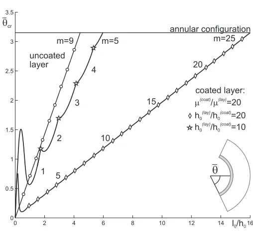
0 2 4 6 8 10 12 14 16 0

0.5 1 1.5 2 2.5 3 3.5

annular configuration

m(coat)/m(lay)=20 coated layer: uncoated

layer

m=5

4

3

2

1

m=25 m=9

5

20

15

10

l /h0 0

qcr

q

h0 / =20 (lay) (coat)

h0

h0 / =10 (lay) (coat)

h0

Figure 4.4: Comparison between the critical angle ¯θcr at bifurcation versus

aspect ratiol0/h0of two neo-Hookean coated bilayers subject to bending with

coating at the compressed side withµ(coat)_/µ(lay)_{= 20 andh}(lay)

0 /h

(coat)

0 = 10

and 20, respectively. In every curve, a small symbol denotes a transition

be-tween two different integer values of m(the parameter which sets the

circum-ferential wavenumber). Bifurcation angles for a single, uncoated layer are also reported.

Some typical finite configurations and stress distributions at bifurcation corresponding tol0/h0= 2 in Figs. 4.1and 4.2 (indicated by small ‘square

symbols’ on the bifurcation curve) are sketched in Fig. 3.2for both positions of the stiff layer.

The critical angle at bifurcation is reported in Figs. 4.3 and 4.4 as a function of the aspect ratio l0/h0 for two values of coating thickness,

h(₀lay)/h(₀coat) ={10, 20}when the coating layer is on the tensile and on the compressive side, respectively. In the same figures the case of the uncoated layer is also reported for comparison. Note that results reported in Fig. 4.3

4.2 Bifurcation of a bilayer

position, though the stiffness ratio between coating and layer is different and equal to 20 in the former case and 500 in the latter. It is evident from the figures that the bifurcation solution for a single layer is approximated by a straight line, so that we can write down the approximated solution

¯

θcr = 0.712l0/h0, (4.23)

which has passed unnoticed until the present work.

We may also notice that a linear relation between ¯θcr and l0/h0 is also

evident in the cases of Figs. 6.1, 4.1, and 4.3, while such a linear relation holds only at high values ofl0/h0in the cases of Figs. 4.2and4.4. Moreover,

the inclination of such lines depends on the elastic and thickness contrasts between layers, so that a simple formula like eqn. (4.23) is hard to be obtained.

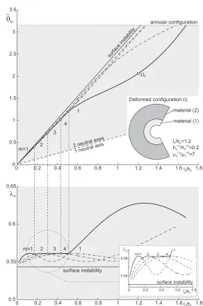
Results for bifurcation of bent configurations for bilayers are presented in Figs. 4.5 and 4.6, in terms of critical semi-angle ¯θcr (upper part) and critical stretch at the compressed side of the specimen [λcr(ri(1)), lower part] as a function of the ‘global’ aspect ratio (the initial length divided by the initial total thickness). The ratios between the thicknesses and the shear coefficientsµ0 of the layers are (1 mm)/(5 mm) and (7 N/mm2)/(1 N/mm2)

for Fig. 4.1, respectively, and (3 mm)/(40 mm) and (2.687 N/mm2)/(0.095 N/mm2) for Fig. 4.2. The various curves reported in Figs. 4.5 and 4.6

represent solutions corresponding to different bifurcation modes, singled out by the circumferential wavenumber m. The mode visible in an experiment is that corresponding to the lower value of the critical semi-angle, ¯θcr, or to the higher value of critical stretch at the compressed side, λcr. Note that the gray zone represents the range of aspect ratios and bending semi-angle for which two neutral axes occur.

analyzed, including Figs. 4.5and4.6, we have found that the gray zone in the ¯

θcr–l0/h0 graphs is bounded by a straight line, becoming a horizontal line in

theλcr–l0/h0 representation. The special feature emerging from Fig. 4.5is

that the modem=1 of bifurcation becomes the critical mode for sufficiently high slenderness, so that here long-wavelength bifurcations (corresponding to small m) become well-separated from surface modes (corresponding to highm) and thus fully visible. This feature is also present in Fig. 4.6, which has been produced with values of parameters corresponding to commercially available rubbers (and tested by me, see Chapter6). In this way it has been possible to produce the two samples shown in Figs. 6.6and6.8, differing only in the aspect ratio (taken equal to 2 for the sample shown in Fig. 6.6 and 1.5 for that shown in Fig. 6.8) and evidencing long-wavelength bifurcation modes.

We provide a justification of the finding that, when two neutral axes occur in a bilayer, the stretch (at the compressed side) is independent of the global aspect ratio l0/h0, so that the gray zone (corresponding to the

presence of two neutral axes) is bounded by a horizontal (inclined) line in theλcr–l0/h0 (in the ¯θcr–l0/h0) representation, Figs. 4.5 and 4.6.

The explanation of this effect is based on two observations. (i.) During progressive bending of a bilayer with the stiff layer under compression, one neutral axis is present from the beginning of the bending within the soft layer, while the second neutral axis always nucleates at the interface between the two layers (and then moves in the stiff layer). (ii.) When the second neutral axis nucleates, the radial Cauchy stressTr at the interface between layers takes a value independent of the initial aspect ratio l0/h0. We can

therefore operate on a single layer by imposing, in addition to the usual bending, a pressurePext _{at one of its external sides (of initial length l}

0) to

4.2 Bifurcation of a bilayer

0.2 0.4 0.6 0.8 1 1.2 1.4 1.6 1.8

0 0.5 0.55 0.6 0.65 0.5 1 1.5 2 2.5 3 3.5 0 0

0.2 0.4 0.6 0.8 1 1.2 1.4 1.6 1.8

0 0.2 0.4 0.6 0.8

0.55 0.56

m=1 2 3

1 4

surface instability

lcr

l /h0 0

m=1 2

4 1

m=1 2 3

3 4 1 surfa ce inst abili ty qcr lcr annular configuration

l /h0 0

l /h0 0

surface instability 2 neutral axes 1 neutral axis W1

Deformed configurationW1

material (1) material (2)

l /h =1.2 h /h =0.2

/ =7 0 0 0 0 0 0 (1) (2) (1) (2) m m

Figure 4.5: Critical angle ¯θcrand critical stretchλcr(evaluated at the internal

boundary, r = ri(1)) versus aspect ratio l0/h0 for a Mooney-Rivlin bilayer

coated with a stiff layer and subject to bending with h(1)0 /h

(2)

0 =(1 mm)/(5

mm) and µ(1)₀ /µ(2)₀ =(7 N/mm2_{)/(1 N/mm}2_{). The stiff layer is located at}

the side in compression. In both plots, a small circle denotes a transition

between two integer values ofm(the parameter which sets the circumferential

wavenumber). In the lower plot, the insert contains a magnification of the

0 1 2 3 4 5 6 7 8 9 0.5 0.55 0.6 0.65 0.7 0.75 0.8 0.85 0.9 0.95

0 1 2 3 4 5 6 7 8 9

0 0.5 1 1.5 2 2.5 3 3.5

0 0.05 0.1 0.15 0.2 0.25 0.54 0.545 0.55 0.555 0.56 0.565 0.57 surface instability

m=1 2 3 4 5

1

lcr

l /h0 0

m=1 2 3 4 5 6 7 8 9

m=1 2 3 4 5 6 7 8 9

l /h0 0

l /h0 0

qcr

lcr

annular configuration

surface instability 1 neutral axis

2 neutral axes 1n eu tral axis 2n eu tral axe s su rface in stab ility

W2 _{Deformed configurationW} 2

material (1) material (2)

l /h =5 h /h =0.075

/ =28.28 0 0 0 0 0 0 (1) (2) (1) (2) m m

Figure 4.6: Critical angle ¯θcrand critical stretchλcr(evaluated at the internal

boundary, r = ri(1)) versus aspect ratio l0/h0 for a Mooney-Rivlin bilayer

coated with a stiff layer and subject to bending with h(1)0 /h

(2)

0 =(3 mm)/(40

mm) andµ(1)0 /µ

(2)

0 =(2.687 N/mm2)/(0.095 N/mm2). The stiff layer is located

at the side in compression. In both plots, a small circle denotes a transition

between two integer values ofm(the parameter which sets the circumferential

wavenumber). In the lower plot, the insert contains a magnification of the

region where bifurcations occur at low l /h . Two neutral axes occur in the

4.2 Bifurcation of a bilayer

To operate in dimensionless form, we introduce, from eqns. (3.9) and (3.13), the kinematic unknowns

¯ α= 2¯θ

a, r¯= r h0

, ¯h= h h0

, (4.24)

where a= l0/h0 is the aspect ratio of the undeformed configuration. The

internal and external non-dimensional radii, from eqn. (3.3), are

¯ ri=

a 2¯θ¯h −

¯ h

2, r¯e = ¯ri+ ¯h. (4.25) As we want to write the bending problem in terms of the variableλi =λ(¯ri), we calculate ¯θas a function of a, ¯h and λi, so that eqn. (3.13)2 gives

¯ θ= a_¯

h

1 ¯ h −λi

, (4.26)

and the condition λe=λ(¯re) becomes λe=

2 ¯

h −λi. (4.27)

The boundary conditions for the layer under consideration are now Tr(¯ri) = 0, Tr(¯re) =Pext, (4.28) where

Tr= µ0

2

λ2+ 1 λ2

+γ,

can be written from eqn. (3.16)1. Eqn. (4.28)2 provides the coefficient γ in

the form

γ =Pext−µ0 2

λ2e+ 1 λ2

e

, (4.29)

while, on the other hand, eqn. (4.28)1 is equivalent to

λ2_i + 1 λ2

i + 2P

ext µ0 − " 2 ¯ h −λi

2

+

2 ¯ h−λi

−2#

0 1 2 3 4 5 6 0

0.5 1 1.5 2 2.5 3 3.5

qcr

annular configuration

l /h0 0

S h /q 0m0

10 1

q

5

Srq=S (u -u )q q q

+

-0 1 2 3 4 5 0

0.5 1 1.5 2 2.5 3

qcr _{annular configuration}

l /h0 0

S h / =1q 0m0 m=1

2 3

4 1

Figure 4.7: Critical angle ¯θcr at bifurcation versus the ‘global’ aspect ratio

l0/h0of two Mooney-Rivlin identical layers jointed through a ‘shear type’

im-perfect interface. The dimensionless stiffness S_{θh0/µ0 takes the values 1, 5,}

and 10. The insert specifies the different values of m (the parameter which

sets the circumferential wavenumber) at bifurcation for S_{θh0/µ0= 1.}

from which it is clear that the unknown ¯his independent of a(but remains dependent onλi,µ0, andPext). Therefore, since a neutral axis corresponds

to

Tθ(¯re) = 0, (4.31) eqns. (3.16)2, (4.29), and (4.27) show that the neutral axis condition is

independent ofa, so that the solution in terms ofλibecomes only a function of µ0 and Pext. The effects of an imperfect interface on bifurcations of a

4.2 Bifurcation of a bilayer

0 1 2 3 4 5 6

0.5 1 1.5 2 2.5 3 3.5

0 1 2 3 4 5 6

0 0.5 1 1.5 2 2.5 3 3.5

annular configuration m=1

annular configuration m=2

S h /q 0m0

S h /q 0m0

l /h0 0 l /h0 0

q q

q

Srq=S (u -u )q q q

+

-q

Srq=S (u -u )q q q

+ -0.1

1 10 50

100 100 50 10 1 0.1

Figure 4.8: Bifurcation angles ¯θ at fixed circumferential number m versus

the ‘global’ aspect ratio l0/h0 for two Mooney-Rivlin identical layers jointed

through a ‘shear type’ imperfect interface as in Fig. 4.7. Left: m=1; right:

m=2. A small number near a curve denotes the value of the dimensionless

stiffness S_θh0/µ0.

and 4.8 pertains to a uniform elastic block divided into two parts through an imperfect interface of dimensionless stiffness S_{θh0/µ0. Note that the}

interface is placed along the initial neutral axis. Results presented in Fig.

4.7 are in terms of the critical bending angle for bifurcation ¯θcr, versus the initial ‘global’ aspect ratio l0/h0, while similar results are reported in Fig.

4.8, but for a fixed circumferential wave number m. Therefore, ¯θ reported in Fig. 4.8 is not ‘critical’, in the sense that it is the bifurcation angle at fixed m, while ¯θcr is the smaller ¯θfor everym.

The results in Figs. 4.7 and 4.8 strongly depend on the dimension-less parameterS_{θh0/µ0representing the interfacial stiffness, which yields an}

5

Numerical procedures to

determine the critical angle

¯

θ

cr

at bifurcation.

5.1

The determinantal method

The bifurcation condition can be numerically determined by introducing, for each layer, the vector

z(r) = [f(r) f0(r) f00(r) f000(r)]T, (5.1) so that the differential eqns. (4.13) can be rewritten as

z0 =N z, (5.2)

where the matrix N takes the form

N =



     

0 1 0 0

0 0 1 0

0 0 0 1

−N41 −N42 −N43 −N44



     

Adopting the notation X(es) =X(s)(r(es)) and X(_is)=X(s)(r_i(s)) for vec-tors or matrices referred to a generic layers, and using eqns. (4.11)–(4.10), the continuity of incremental tractions and displacements at an interface between layers, eqns. (4.15), can be represented in matrix form as

h

Q(es) −Q(_is+1)

i 



z(es) z(_is+1)



=0, (5.4)

where

Q(r) =



     

F(n2_{−1) r[F−n}2_(2D+C−T

r)] r2(F + 3C) r3C (n2_−1)(C−T

r) r(C+Tr) r2C 0

1 0 0 0

1 r 0 0



     

,

(5.5) while boundary conditions (4.20) can conveniently be rewritten as

P_i(1) z(1)_i =0, P_e(N) z(_eN)=0, (5.6) where

P(r) =





F(n2−1) r[F−n2(2D+C)] r2(F + 3C) r3C

n2−1 r r2 0



. (5.7)

We are now in a position to set the numerical solution procedure. Since in our examples we have always addressed systems with few layers, we use the simple following numerical procedure.

1) Employing a numerical integration based on an explicit Runge-Kutta (4,5)-formula, we solve, for each layer (index s has been dropped for simplicity), four initial-value problems. These are based on system (5.2), with the following four initial conditions:

5.1 The determinantal method

z_(3)i = [0 0 1 0]T, z_(4)i = [0 0 0 1]T. In this way, we find four integrals,

z_(m)(r) (m= 1, . . . ,4), (5.8) for each layer.

2) The general solution for each layer can be constructed by linear com-bination of the four functions (5.8), so that we obtain

z(r) =C1z(1)(r) +C2z(2)(r) +C3z(3)(r) +C4z(4)(r), (5.9)

where the unknown constants Ci (i = 1, . . . ,4) set the amplitude of the bifurcation mode. These can be collected for each layer in a vector c= [C1 C2 C3 C4]T.

3) Boundary and interfacial conditions for the multilayer can be recast in matrix form as

               ˆ

P(1)_i : 0

ˆ

Q(1)_e −Qˆ(2)_i : ˆ Q(1)_e :

.. .. .. .. ..

: Qˆ(_eN−1) −Qˆ(_iN)

0 : Pˆ(_eN)

                             c(1) c(2) .. ..

c(N−1)

c(N)

             

=0, (5.10)

or equivalently as

¯

Wˆc=0, (5.11)

where

ˆ P(_i,es) =



 

P₁(_js)z₍₁₎(s)_j P₁(s_j)z(₍₂₎s)_j P₁(_js)z₍₃₎(s)_j P₁(_js)z₍₄₎(s)_j

P₂(_js)z₍₁₎(s)_j P₂(s_j)z(₍₂₎s)_j P₂(_js)z₍₃₎(s)_j P₂(_js)z₍₄₎(s)_j



 

r=ri,re

and

ˆ Q(_i,es)=



          

Q(₁s_j)z(₍₁₎s)_j Q(₁s_j)z₍₂₎(s)_j Q(₁s_j)z₍₃₎(s)_j Q(₁s_j)z₍₄₎(s)_j

Q(₂s_j)z(₍₁₎s)_j Q(₂s_j)z₍₂₎(s)_j Q(₂s_j)z₍₃₎(s)_j Q(₂s_j)z₍₄₎(s)_j

Q(₃s_j)z(₍₁₎s)_j Q(₃s_j)z₍₂₎(s)_j Q(₃s_j)z₍₃₎(s)_j Q(₃s_j)z₍₄₎(s)_j

Q(₄s_j)z(₍₁₎s)_j Q(₄s_j)z₍₂₎(s)_j Q(₄s_j)z₍₃₎(s)_j Q(₄s_j)z₍₄₎(s)_j



          

r=ri,re

, (5.13)

so that bifurcation corresponds to the condition that system (5.10) admits a non-trivial solution, namely,

det ¯W = 0, (5.14)

which provides the critical semi-angle ¯θcr.

5.2

The compound matrix method for a bilayer

The compound matrix method was initially proposed by Backus and Gilbert, Ref.[4], and applied to problems of fluid mechanics, Refs.[3,36–38,56], and solid mechanics, Refs. [32, 33]. Haughton and Orr, Ref. [29], used the method in incremental elasticity, while Refs. [18,19,22,28] employed it to investigate instabilities of a homogeneous block subjected to finite flexure. Our aim is to show the application to elastic multilayers subject to finite bending in the simple case of a bilayer.

The differential equation (4.13) can be re-written as a linear system of first-order ODEs, that in the case of two elastic layers can be cast in the following standard form

y0 =Ay,

z0=B z, (5.15)

where vectorsy and z are defined as

y(r) = [f(1)(r) f(1)0(r) f(1)00(r) f(1)000(r)]T,

5.2 The compound matrix method for a bilayer

and matrices Aand B, which depend on the radial coordinate r, as

A(r) =

      

0 1 0 0

0 0 1 0

0 0 0 1

A41 A42 A43 A44

      

, B(r) =

      

0 1 0 0

0 0 1 0

0 0 0 1

B41 B42 B43 B44

       . (5.17) The components ofA andB, as well as those of other matrices and vectors introduced in this Chapter are listed in Appendix A.

The boundary conditions at the two external surfaces of the layer, eqns. (4.20), are equivalent to

C y(ri) =0, D z(re) =0, (5.18) where ri =ri(1),re=ri(2)+h(2) and matrices C and D are

C =





C11 C12 C13 C14

C21 C22 C23 0



, D =





D11 D12 D13 D14

D21 D22 D23 0



.

(5.19) Continuity conditions between the two layers, eqns. (4.15), can be written as

Gy(rm) +H z(rm) =0, (5.20) where rm=ri(1)+h(1) and matrices G and H are defined as

G=       

G11 G12 G13 G14

G21 G22 G23 0

G31 0 0 0

G41 G42 0 0

      

, H =

      

H11 H12 H13 H14

H21 H22 H23 0

H31 0 0 0

H41 H42 0 0

interface conditions (5.21)] into two matrices sharing the following common structure        ∗I

1 ∗II1

∗I

2 ∗II2

∗I

3 ∗II3

∗I

4 ∗II4

       , (5.22)

(where the symbol ‘∗’ stands for either y or z) and defining the so-called ‘compound matrices’. Moreover, we introduce the vectors φy_i (i = 1, ...,6) and φz_i (i = 1, ...,6) collecting the components of the minors of matrices (5.22) as

φ∗

1 =∗I1∗II2 − ∗I2∗II1 , φ∗4=∗I2∗II3 − ∗I3∗II2 ,

φ∗

2 =∗I1∗II3 − ∗I3∗II1 , φ∗5=∗I2∗II4 − ∗I4∗II2 ,

φ∗

3 =∗I1∗II4 − ∗I4∗II1 , φ∗6=∗I3∗II4 − ∗I4∗II3 .

(5.23)

With the definitions (5.22) and (5.23), the differential problem (5.15) can be shown (Ref. [36]) to be equivalent to the new problem

(φy)0=MAφy, (φz)0=MBφz, (5.24)

where, introducing the symbol ‘’, equal to A (to B) for φy (for φz), we define

M=

           

0 1 0 0 0 0

0 0 1 1 0 0

42 43 44 0 1 0

0 1 0 0 1 0

−41 0 0 43 44 1

0 −41 0 −42 0 44

            . (5.25)

The system of differential eqns. (5.24) has to be solved using a Runge-Kutta (4,5) numerical method (we have used MatlabR _{ver. 7.9) to determine}

5.2 The compound matrix method for a bilayer

The solution of the bifurcation problem can be written as a linear com-bination of the solutions yI,yII,zI, and zII,

y =ξ1yI +ξ2yII,

z =ξ3zI +ξ4zII,

(5.26)

where the arbitrary coefficients ξi (i = 1, ...,4), which set the amplitude of the bifurcation mode, remain undefined in a linearized analysis. The conditions at the internal interface (5.20) can be recast as

Wξ=0, with ξ = [ξ1 ξ2 ξ3 ξ4]T, (5.27)

where W =          GyI 1 GyII 1

H zI

1

H zII

1 GyI 2 GyII 2

H zI

2

H zII

2 GyI 3 GyII 3

H zI

3

H zII

3 GyI 4 GyII 4

H zI

4

H zII

4          , (5.28)

so that the bifurcation condition, depending on the bending semiangle ¯θ, the undeformed aspect ratios l0/h0 and h(1)0 /h

(2)

0 , and the stiffness ratio

µ(1)₀ /µ(2)₀ , becomes

det(W) = 0. (5.29)

Condition (5.29) can be rewritten as the sum of 2×2-determinants as

1 X i=0 (−1)i   

W1+i,1 W1+i,2

W41 W42

W2−i,3 W2−i,4

W33 W34

−

W2+i,1 W2+i,2

W11 W12

W3−i,3 W3−i,4

W43 W44

−

W2+2i,1 W2+2i,2

W31 W32

W4−2i,3 W4−2i,4

W13 W14

  

= 0.

0.2 0.22 0.24 0.26 0.28 -8 -6 -4 -2 0 2 4

x 1044

q Det( ) M compound matrix method determinantal method

Figure 5.1: The compound matrix method (dashed line) against the

de-terminantal method (solid line): det(M) is evaluated at different angles ¯θ,

for l0/h0 =0.1, h(1)0 /h (2)

0 =(1 mm)/(5 mm) and µ

(1)

0 /µ

(2)

0 =(7 N/mm2)/(1

N/mm2). Bifurcation corresponds to the vanishing of det(M); note the

‘spu-rious’ oscillations of the latter method.

The determinants can be expressed in terms of the wctors φy and φz as

Wk1 Wk2

Wl1 Wl2

= (Gk1Gl2−Gk2Gl1)φy1+ (Gk1Gl3−Gk3Gl1)φy2

+(Gk1Gl4−Gk4Gl1)φy3+ (Gk2Gl3−Gk3Gl2)φy4

+(Gk2Gl4−Gk4Gl2)φy5+ (Gk3gl4−Gk4Gl3)φy6,

(5.31) and

Wk3 Wk4

Wl3 Wl4

= (Hk1Hl2−Hk2Hl1)φz1+ (Hk1Hl3−Hk3Hl1)φz2

+(Hk1Hl4−Hk4Hl1)φz3+ (Hk2Hl3−Hk3Hl2)φz4

+(Hk2Hl4−Hk4Hl2)φz5+ (Hk3Hl4−Hk4Hl3)φz6,

(5.32) in which indiceskandltake the values corresponding to the representation (5.30). Once the undeformed aspect ratiosl0/h0 andh(1)0 /h

(2)

0 and the

5.2 The compound matrix method for a bilayer

representation (5.30), becomes a function of the bending semiangle ¯θ only, to be solved numerically (we have used the function ‘fzero’ of MatlabR _ver.

7.9). An example of the advantage related to the use of the compound ma-trix method over the ‘usual’ determinantal method is reported in Fig. 5.1, where det(W) is plotted as a function of ¯θ for a ‘stiff’ case, in which the superiority of the former approach is evident (note the ‘spurious’ oscillations of the determinantal method). In this particular case, the 2-norm condition number of the matrixW is equal to 9.37×1027_{, a value confirming that the}

6

Experiments on coated and

uncoated rubber blocks

under bending

To substantiate the theoretical results on bifurcation of layered structures subject to finite bending, Roccabianca et al. (Refs. [43] and [44]) have de-signed and performed experiments, in the way initiated by Gent and Cho (Refs. [26] and [25]). In particular, we have imposed a finite bending to uncoated and coated elastic strips (made of natural rubber), employing the device shown in Fig. 6.2, in which a rubber strip is glued to two metal-lic platelets along the longer sides (using Loctitec_{) and these platelets are}

forced to impose a bending to the strip, using a simple screw-loading de-vice. Two different coatings have been tested, both realized using 0.2 mm thick polyester transparent films (commercial copier films), glued singular or double (using Loctitec_{) to the rubber strip. During finite bending, the}

appearance of crazes has been detected by direct visual inspection.

m(coat)m(lay) / =500

0 2 4 6 8 10 12 14 16 18

0 0.5 1 1.5 2 2.5 3 3.5

qcr annular configuration

l /h0 0 uncoated

layer

experiment:

experiment: uncoated

h(lay)/h(coat)=20

0 0

experiment: h(lay)/h(coat)=10

0 0

W1 W2

W3

W5

coated layer:

h(lay)/h(coat)=20

0 0

h(lay)/h(coat)=10

0 0

W1 W2 W4 W5

m=12 m=11

m=9

8

7

5

4

3

2

1

W3 W4

Figure 6.1: Experimental results versus theoretical predictions for the

bifur-cation opening semi-angle ¯θcr of uncoated and coated rubber strips subject to

finite bending, versus the aspect ratiol0/h0 of the undeformed configuration.

The shear moduli ratioµ(coat)_/µ(lay)_{of the coated layers has been taken equal}

to 500, while two thickness ratios h(lay)₀ /h(coat)₀ equal to 20 and 10 have been

considered. The critical theoretical configurations (forh(lay)0 /h

(coat)

0 = 20)

cor-responding to bifurcation points Ωi(i= 1, . . . ,4) are sketched in the right part

rubber block

scale for bending angle measure screw loading device

Figure 6.2: Device used to impose finite bending (of a semi-angle ¯θ equal to

25◦ _{on the left and to 45}◦ _{on the right, with reference to Fig. 3.1) to coated}

and uncoated rubber strips (an uncoated 10 mm ×100 mm ×4 mm rubber

strip is subject to bending in the photo).

0 10 20 30 40 50 60

1 1,05 1,1 1,15

0 5 10 15 20

1 2 3 4 5

70

T

ruestress[kN/mm

]

2

T

ruestress[kN/mm

]

2

stretch range of interest

neo-Hookean interpolation range of interest

neo-Hookean interpolation

stretch

where the true stress is plotted versus the stretch. It may be interesting to note that, while the response of the rubber is typical of these materials, the stress/stretch curve of the polyester film is highly nonlinear, exhibit-ing a peak and a softenexhibit-ing regime. In the plots, the interpolation with the neo-Hookean material selected for the calculations is also included (giving µ(lay) ' 1 kN/mm2 and µ(coat) ' 500 kN/mm2). This interpolation curve may seem poor at a first glance, but we should point out that all the bi-furcations found in the experiments have occurred with maximum stretches ranging between 1.52 and 1.9 (1.38 and 1.64 for samples with thick coating) in the rubber and between 1.02 and 1.04 (1.01 and 1.02 for samples with thick coating) in the polyester. For this reason, the selected neo-Hookean interpolation is much more accurate than it may appear and is taken valid either in tension or in compression. The prog