R E V I E W
Open Access
DYAMOND: the DYnamics of the
Atmospheric general circulation Modeled On
Non-hydrostatic Domains
Bjorn Stevens
1*, Masaki Satoh
2, Ludovic Auger
3, Joachim Biercamp
4, Christopher S. Bretherton
5,
Xi Chen
6, Peter Düben
7, Falko Judt
8, Marat Khairoutdinov
9, Daniel Klocke
10, Chihiro Kodama
11,
Luis Kornblueh
1, Shian-Jiann Lin
6, Philipp Neumann
4, William M. Putman
12, Niklas Röber
4,
Ryosuke Shibuya
11, Benoit Vanniere
13, Pier Luigi Vidale
13, Nils Wedi
7and Linjiong Zhou
6Abstract
A review of the experimental protocol and motivation for DYAMOND, the first intercomparison project of global storm-resolving models, is presented. Nine models submitted simulation output for a 40-day (1 August–10
September 2016) intercomparison period. Eight of these employed a tiling of the sphere that was uniformly less than 5 km. By resolving the transient dynamics of convective storms in the tropics, global storm-resolving models remove the need to parameterize tropical deep convection, providing a fundamentally more sound representation of the climate system and a more natural link to commensurately high-resolution data from satellite-borne sensors. The models and some basic characteristics of their output are described in more detail, as is the availability and planned use of this output for future scientific study. Tropically and zonally averaged energy budgets, precipitable water distributions, and precipitation from the model ensemble are evaluated, as is their representation of tropical cyclones and the predictability of column water vapor, the latter being important for tropical weather.
Keywords: Climate modeling, Model intercomparison project, Tropical convection, Convective parameterization
Introduction
About 20 years ago, Taroh Matsuno proposed to develop a global non-hydrostatic model as a demonstrator project for the Earth Simulator, a Japanese supercomputer that was being developed to be the most powerful of the world at that time (Matsuno2016). His idea was to pro-vide a tropical analogue to the mid-latitude numerical experiments of Phillips (1956) and Smagorinsky (1963)— one that could resolve the transient dynamics of tropi-cal deep convection, and its various forms of organiza-tion. Doing so required a global grid, and a formulation of the governing equations, that would permit motions on scales of 5 km. Such approaches, long common place on smaller domains1, became conceivable globally
*Correspondence:[email protected]
1Max Planck Institute for Meteorology, Bundesstraße 53, 20146, Hamburg,
Germany
Full list of author information is available at the end of the article
1By the early 2000s, approaches pioneered by Cotton and Tripoli (1978) and
Klemp and Wilhelmson (1978) had become operational (Saito et al.2007).
with the ambitious development of the Earth Simulator (Satoh et al.2005). These efforts bore fruit, in the form of new numerical methods (Tomita et al. 2001; Tomita and Satoh 2004) and the first ever aqua-planet simula-tions using a global non-hydrostatic model called NICAM (Tomita et al.2005; Satoh et al.2008; Satoh et al.2014). NICAM, which has since been applied to more realistic planetary configurations and a great variety of questions (see reviews by Satoh et al. 2017, 2018, 2019), demon-strated the ability of a model to use unfiltered equations of atmospheric motion, on a global domain, to represent convective storms in the tropics as a component of the general circulation.
In the years since the introduction of NICAM, a small number of groups initiated similar efforts to use the continuing growth in computational capacity (e.g., Putman and Suarez (2011)) to enable the simulation of the atmospheric general circulation on non-hydrostatic domains (Satoh et al.2019). These groups, coming from
different modeling traditions—weather prediction, data assimilation, mesoscale meteorology, and climate sci-ence, shared a common purpose. By explicitly simulating how small and intermediate scales of motions couple to large-scale circulation systems, they sought to circumvent considerable, and seemingly intractable, problems arising from parameterizations—particularly of deep convection (Randall et al. 2003; Stevens and Bony 2013). Mod-els with this capacity—which we call global storm-resolving models (or GSRMs)—are providing the foun-dation for a new generation of weather and climate models. Their use will shine welcome new light on long-standing questions, such as how tropical rainbands, or other patterns of weather, change with warming (Bony et al.2015; Marotzke et al.2017).
An important next step in the application of such mod-els is to begin identifying which aspects of the simu-lated climate system are independent of the details of the GSRM implementation. Separating robust (implementa-tion independent) from non-robust features is most easily done through a controlled program of model intercom-parison. Such an intercomparison helps shape expecta-tions and guide future developments in at least three ways: (i) by identifying and helping resolve what should be trivial problems, such as apparent implementation bugs; (ii) by focusing efforts on non-trivial problems, for instance the representation of turbulent mixing and cloud microphysical processes, or managing and effi-ciently analyzing output; and (iii) by involving a larger community in the excitement of exploring the behav-iors of a new class of models. Toward these ends, we have initiated the first intercomparison of GSRMs, through a project we call DYAMOND—the DYnamics of the Atmospheric general circulation On Non-hydrostatic Domains2.
The aim of this paper is to describe DYAMOND and present first results. The selection of what to present was guided by a desire to illustrate promising directions of analysis that have emerged from initial explorations of the output, and to make a first identification of issues for the further development of this simulation capability. To accomplish our aim the remainder of this paper is orga-nized as follows: The DYAMOND experimental protocol is presented in the “Experimental protocol” section. In the “Models” section, we present the nine models which contributed simulation output to DYAMOND, including some characteristics of their computational performance and a brief description of the output they provide. In the “Simulations” section some characteristics of the simula-tions are presented by way of overview, complemented by snapshots to help motivate subsequent work by a broader
2https://www.esiwace.eu/services/dyamond
community. We conclude with a summary and our ideas regarding future steps.
Experimental protocol
The DYAMOND protocol specified a simulation of 40 days and 40 nights, beginning at 0Z, 1 August 2016, using global models with a grid spacing of 5 km or less. The global (9 km) meteorological analysis taken from the European Centre for Medium Range Weather Fore-casts (ECMWF) was used to initialize the atmospheric state. ECMWF operational daily sea-surface tempera-tures and sea-ice concentrations were also used as initial and boundary data. These input fields are archived and made available as part of the DYAMOND dataset. Mod-els were left free to formulate their own initialization of the land surface and adopted a variety of strategies for this purpose. ICON, for instance, took soil mois-ture from ECMWF and converted to a soil moismois-ture index (SMI) which was then vertically interpolated to the ICON soil level SMI and soil temperature which it then converted back to soil moisture using ICON’s soil char-acteristics. MPAS used the NOAH-MP land model and initialized it with ERA5 surface data from 1 August 2018, and other models, such as the UKMO, used soil mois-ture taken from previous, lower-resolution runs. Perhaps because the resolution of the analyses used for initial-ization was relatively fine, no groups reported special problems with the initialization, even if spurious gravity waves are expected to arise from topographic and other mismatches.
The initialization date (1 August 2016) was motivated by the possibility of linking to previous large-domain storm-resolving model simulations performed in support of field work over the Northern Atlantic (Klocke et al.
2017; Stevens et al.2019). The coincidence of this period with the boreal monsoon, the active part of northern hemispheric tropical cyclone season, and the good satel-lite coverage were further motivations. Simulating 40 days and 40 nights had a symbolic motivation, as in some ancient cultures it denotes an eternity, and a practical motivation, as it allowed for a comparison of 30 days (1 month) after a 10-day spin-up. Through this, it was hoped to crudely separate questions of predictability from questions of climatology.
Models
Structure and configuration
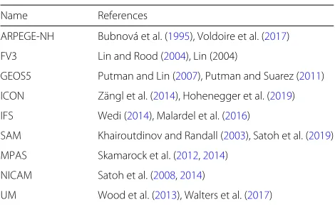
Most of the DYAMOND models (Table1) solve the fully compressible Navier-Stokes equations, with their repre-sentation of molecular diffusion modified to account for unresolved turbulent motions and for an atmosphere with a condensible (water) component. Exceptions are the Sys-tem for Atmospheric Modeling (SAM) which uses the anelastic form of the non-hydrostatic equations and the Integrated Forecast System (IFS) which uses the (hydro-static) primitive equations and is thus the only hydrostatic model. More generally, the numerical methods used by the different models to solve their governing equations depend on their choice of grid and a number of other factors, and thus vary considerably. These differences contribute to the richness of the simulation dataset as a basis for assessing the importance of model formula-tion choices. Table1provides technical references for the participating models.
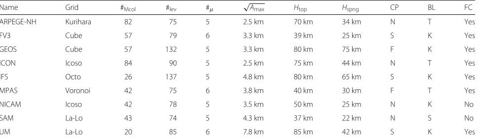
The configuration of the numerical grid over which each model solves its governing equations, and some param-eters indicative of how these equations are structured, is given in Table2. A diversity of grids—many of which are
Table 1DYAMOND models
Name References
ARPEGE-NH Bubnová et al. (1995), Voldoire et al. (2017)
FV3 Lin and Rood (2004), Lin (2004)
GEOS5 Putman and Lin (2007), Putman and Suarez (2011)
ICON Zängl et al. (2014), Hohenegger et al. (2019)
IFS Wedi (2014), Malardel et al. (2016)
SAM Khairoutdinov and Randall (2003), Satoh et al. (2019)
MPAS Skamarock et al. (2012,2014)
NICAM Satoh et al. (2008,2014)
UM Wood et al. (2013), Walters et al. (2017)
Short names for models submitting output to DYAMOND and references to recent scientific documentation for each model
reviewed by Williamson (2007)—are employed across the DYAMOND models. FV3 and GEOS5 share a dynamical core based on a cubed sphere, NICAM and ICON use an icosahedral grid as a starting point for their discretization, and MPAS employs spherical centroidal Voronoi tessella-tion. The IFS operates with a cubic octahedral (Gaussian) reduced grid with T2559 truncation in spectral space, and the ARPEGE-NH uses an alternative Gaussian reduced grid with the truncation T8000 in spectral space. The UM and SAM use latitude-longitude grids, which introduce more severe numerical challenges as they are refined. For SAM, as it was implemented for DYAMOND, a columnar (wall) boundary pierces the sphere and bounds the flow to lie equatorward of 89◦latitude. For the UM, no special accommodation for the pole was introduced except to use a somewhat coarser tiling of the sphere (see Table2) as compared to the other models.
The DYAMOND models differ more substantially in their choice of vertical coordinates, thermodynamic vari-ables, and how parameterizations are used to represent processes that would otherwise be inadequately repre-sented. Table 2 also gives a flavor of these differences; more detailed descriptions are provided in each model’s technical documentation (Table1). Notably models dif-fered in how they treated convective parameterization, especially shallow convection, perhaps reflecting a lack of consensus as to how much of the convection would be explicitly resolved at the target grid spacing.
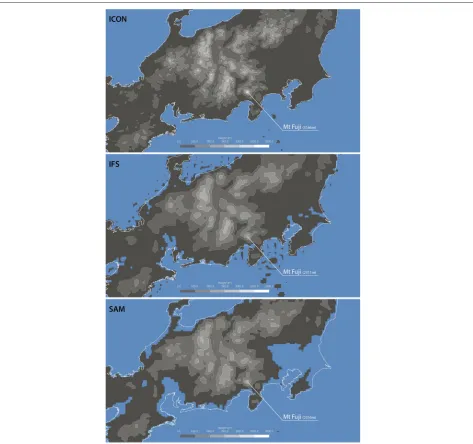
The choice of vertical coordinate influences the stabil-ity of the model in regions of steep topography and the representation of the topography itself. Figure1visualizes a subset of the DYAMOND models in the vicinity of Mt. Fuji to illustrate these differences. It emphasizes that the number of levels is not the only consideration when eval-uating the vertical resolution among the different models. Differences in the surface orography manifest themselves not only in the height and steepness of mountains, but also on the shape of the coastline, and the extent to which some features (small islands) are even represented.
The vertical span of the model grids and the number of levels over which they are discretized also vary (Table2), and most models employ some form of damping as their upper boundary is approached. For example, in the case of ICON, this damping is applied to the levels between 44 km and the model top, which is at 75 km.
Output
Table 2Configuration of the DYAMOND models
Name Grid #Mcol #lev #μ √Amax Htop Hspng CP BL FC
ARPEGE-NH Kurihara 82 75 5 2.5 km 70 km 34 km N T Yes
FV3 Cube 57 79 6 3.3 km 39 km 25 km S K Yes
GEOS Cube 57 132 5 3.3 km 80 km 75 km F K Yes
ICON Icoso 84 90 5 2.5 km 75 km 44 km N T Yes
IFS Octo 26 137 5 4.8 km 80 km 65 km S K Yes
MPAS Voronoi 42 75 6 3.8 km 40 km 30 km F T Yes
NICAM Icoso 42 78 5 3.5 km 50 km 25 km N K No
SAM La-Lo 43 74 5 4.3 km 37 km 22 km N S No
UM La-Lo 20 85 6 7.8 km 85 km 42 km S K Yes
Tabulated are the number of columns (#Mcol, in millions), the vertical levels (#lev, not counting soil levels), the microphysical variables (#μ), the linear dimension of the area, theAof the largest tile (√Amax), the vertical span of the column (Htop), and the height (Hspng) where the sponge layer begins. The last three columns denote
parameterization assumptions. For cumulus parameterization (denoted CP), the letters “N,” “S,” and “F” denote none, shallow, or full parameterization, whereby for the latter, some assumptions are usually included in an attempt to account for the scale of motions being parameterized. For the boundary layer parameterization (denoted BL), the letters “T,” “K,” and “S” denote either a TKE-like model (including an additional prognostic equation), a diagnostic eddy diffusivity, or a Smagorinsky-like three-dimensional closure as is common for large-eddy simulation. Finally, some indication is given as to whether fractional cloudiness (denoted FC) is parameterized
nearly a terabyte of information (664 GBytes, double pre-cision) per sample. Hourly output for 40 days inflates this by a factor of a thousand. The practice of provid-ing derived variables, e.g., measurprovid-ing energy and mat-ter fluxes, inflates this by another factor of 3. Hence, approaching the output naively would imply data vol-umes of about 2 PBytes for each model. This contex-tualizes one motivation for DYAMOND, which was to develop strategies for dealing effectively with the large amount of information inherent in GSRMs. For this rea-son, groups were encouraged to approach the problem as they saw fit, with the idea that the sharing of approaches would help guide the development and uptake of best practices.
All groups used a hierarchical approach, with more fre-quent output of 2D variables and less frefre-quent output of 3D fields. Most groups limited 3D output to a fairly small elaboration of their state vector at 3 h intervals. Some two-dimensional output was written to disk by most models every 15 min, every 30 min for SAM, and every 60 min for the IFS. To avoid unnecessary repetition in output, many models, usually those with a less regular grid structure (i.e., ICON, FV3, and MPAS), provided grid information in a stand-alone file which must be specified when read-ing the data. NICAM and GEOS fall into this category, but only distributed output after it had been remapped to a regular grid. All groups provided output in some flavor of GRIB or NetCDF, and many groups employed some form of compression before writing output to disk. Compres-sion saves space, but slows access to the data, which must be decompressed before use. This issue was especially evi-dent when accessing ICON output, which was written using the GRIB2 standard and a second level of compres-sion. This approach reduced the output file volumes by
a factor of 5, but because the second-level decompres-sion did not multi-thread well, access to the output was considerably slower. This experience has since motivated task-parallel optimization developments to improve the decompression step, but is a reminder that compressed formats involve trade-offs.
The simulations provide a lot of samples of mesoscale convective systems, whose statistical characteristics can be analyzed. To aid exploration of the output, a stan-dardized set of (two-dimensional) information (Table 3) was post-processed for each model. The processing con-sisted of interpolating the variables to a common 0.1◦ grid (using a conservative remapping via the remap func-tion of CDO version 1.9.5) and saving, for each time level of each model’s output, the data as a netCDF (ver-sion 4) file. The remapped output of model variables was averaged over the full 40-day period, as well as over the last 30, 20, and 10 days, leading to 4 time-averaged output files on the same 0.1◦ grid for each model. To ensure consistency between the remapped and source output, and because the number of participating mod-els is small, the data provided on the 0.1◦ grid retain the same variable name, and units, as the original model output.
The sheer size of the output fields also poses quite a challenge for their visualization. Even in the cases where we might be able to visualize model output using rel-atively conventional approaches, to interactively explore and visually analyze the full 3D data set over time, would require parallel visualization techniques. For yet larger simulations, in situ visualization techniques and/or an online compression and a level-of-detail (LoD) rendering approach (Jubair et al.2016; Bethel et al.2012; Clyne et al.
Fig. 1Orographic boundary conditions around the region of Mt. Fuji (3776 m). Plotted is the height of the surface, relative to mean sea level, taken from ICON, IFS, and SAM to illustrate different representations of topography. Note that the land-sea mask does not correspond to the height of the 0 m contour, so even if regions may formally be just above, respectively below, sea level, this does not preclude them from being treated as sea, respectively land
The German Climate Computing Center (DKRZ) agreed to host the output and serve as an analysis hub for the community, something made possible through close interaction with a European Commission funded Centre of Excellence in Simulation of Weather and Climate in Europe—the ESiWACE project.
An accidental ensemble
There is a temptation to question what can be learned about the climate system from a single 40-day snapshot.
Experience suggests a great deal. For instance, Rodwell and Palmer (2007) showed how initial tendency errors— identified in a data-assimilation procedure—are informa-tive of model biases. Simpler approaches, using hindcasts, have shown to be similarly indicative of climatological biases (Williamson2005; Williams et al.2013).
Table 3Homogenized output variables
Quantity
Precipitation (rate) at the surface
Column integrated total water
Column integrated liquid water
Column integrated solid water (ice)
Net terrestrial radiation (at TOA and surface)
Net TOA solar radiation (at TOA and surface)
Pressure (interpolated to sea level)
Zonal wind speed (at 10 m)
Meridional wind speed (at 10 m)
Temperature (at 2 m)
Each model’s variables were remapped to a regular 2D LaLo grid, and these were in turn time-averaged for four different periods. The remapping was done to ensure that, at a minimum, the following information was available for each model
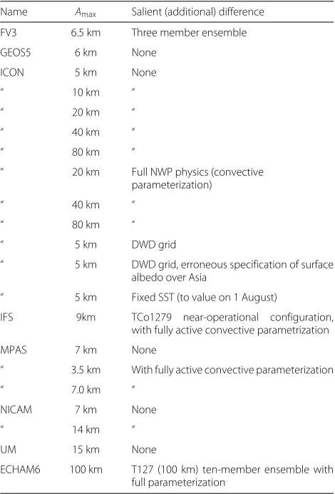
of additional simulations. These include simulations per-formed with the identical model but at progressively lower resolution, simulations with different parameter settings, and simulations with what was later deemed to be unde-sirable treatments of boundary or initial data. Table 4
describes the additional DYAMOND simulations that have been archived and made available as part of this ensemble. So for instance based on this table, simply by comparing an ICON simulation run at 5 km with a sim-ulation run in the base configuration and comparing it to another model run at its base configuration, one can begin to assess to what extent differences between the models are likely to be systematic.
Computational performance
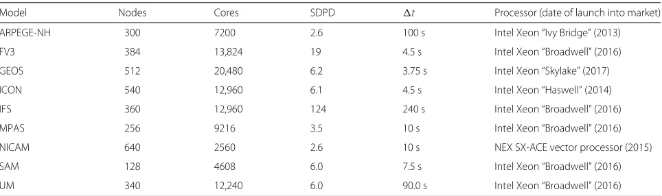
To aid efforts to assess (and eventually enhance) the com-putational efficiency of GSRMs, groups were asked to specify some computational details of their calculations. These are provided in Table 5. The information in the table is difficult to interpret without expertise in the dif-ferent computational architectures on which the models were run. It is also colored by the different levels of effort groups have put into optimizing the porting of their model to their particular computing environment. The struc-ture of the model itself also influences the interpretation of these numbers; for instance, most models use differ-ent time-integration schemes, or differdiffer-ent timesteps, for marching different processes forward in time. Because it usually sets the pace, the shortest timestep (usu-ally used to represent sound waves) is also listed in Table5.
Notwithstanding these caveats, some general conclu-sions can be drawn. One is that the throughput of the DYAMOND models on a O(3 km) mesh was about 6 SDPD (simulated days per day) on a modest frac-tion of the host-machine nodes (ICON was run on one
Table 4Accidental ensemble
Name Amax Salient (additional) difference
FV3 6.5 km Three member ensemble
GEOS5 6 km None
ICON 5 km None
“ 10 km “
“ 20 km “
“ 40 km “
“ 80 km “
“ 20 km Full NWP physics (convective
parameterization)
“ 40 km “
“ 80 km “
“ 5 km DWD grid
“ 5 km DWD grid, erroneous specification of surface albedo over Asia
“ 5 km Fixed SST (to value on 1 August)
IFS 9km TCo1279 near-operational configuration,
with fully active convective parametrization
MPAS 7 km None
“ 3.5 km With fully active convective parameterization
“ 7.0 km “
NICAM 7 km None
“ 14 km “
UM 15 km None
ECHAM6 100 km T127 (100 km) ten-member ensemble with full parameterization
Salient information about additional simulations performed by various groups and made available as part of the DYAMOND archive
sixth of the DKRZ machine Mistral). IFS, representing a large class of existing global numerical weather predic-tion models (Mengaldo et al.2018), operates at a higher SDPD, in part due to the numerical scheme allowing the stable use of larger timesteps and the use of single pre-cision. Similar time-stepping procedures were used by the UM and ARPEGE-NH, but did not permit as large a timestep as was possible for the hydrostatic imple-mentation of the IFS. With increasing vertical accelera-tions, some of the numerical simplifications that enable a large throughput for models like the IFS come into ques-tion. Results made available by DYAMOND will foster research on the numerical and algorithmic trade-offs on scales where non-hydrostatic accelerations may become important.
Table 5Computational aspects
Model Nodes Cores SDPD t Processor (date of launch into market)
ARPEGE-NH 300 7200 2.6 100 s Intel Xeon “Ivy Bridge” (2013)
FV3 384 13,824 19 4.5 s Intel Xeon “Broadwell” (2016)
GEOS 512 20,480 6.2 3.75 s Intel Xeon “Skylake” (2017)
ICON 540 12,960 6.1 4.5 s Intel Xeon “Haswell” (2014)
IFS 360 12,960 124 240 s Intel Xeon “Broadwell” (2016)
MPAS 256 9216 3.5 10 s Intel Xeon “Broadwell” (2016)
NICAM 640 2560 2.6 10 s NEX SX-ACE vector processor (2015)
SAM 128 4608 6.0 7.5 s Intel Xeon “Broadwell” (2016)
UM 340 12,240 6.0 90.0 s Intel Xeon “Broadwell” (2016)
To give a rough idea of the performance of the different models, their throughput is given and contextualized by some basic information about architectures on which they were run. Columns indicate the number of nodes, the total number of cores on which the simulations were run, the simulated days per day, the shortest (usually acoustic) timestep (t), and the type of processor
element at the given limited core counts; most mod-els typically have a column-to-processing-element ratio of about 104. From this, we conclude that even without confronting disruptive changes that stand in the way of achieving yet greater gains, a factor of 10 to 15 in compu-tational throughput in a 5-year period will be achievable. Such an increase would enable global simulations on a 3-km grid with throughput of about 100 SDPD and hence allow these approaches to be applied to a broader class of climate change questions. It also makes global LES, with simulations of a few days on a 300-m grid, conceiv-able. The latter could be used to target some of the— not inconsiderable—simulation uncertainties that remain in GSRMs, since fully resolving shallow cloud systems, whose vertical (and hence horizontal) scale may be only a few kilometers, requires substantially smaller grid distances.
Simulations “Palmer-Turing” test
In an essay on modeling the climate system, Palmer (2016) introduced the notion of using Alan Turing’s test as a mea-sure of climate model fidelity. Turing’s original idea was to use the extent to which a passive observer could dis-tinguish a conversation between a human and a computer from a conversation between two humans as a measure of artificial intelligence. Palmer’s variant of Turing’s test is presented in Fig.2, which compares a snapshot of the Earth from a geostationary satellite, with a visualization of its condensate burdens using output from the nine DYA-MOND models. A second simulation by the IFS, at its operational resolution, is also included as a further refer-ence. The visualizations are created using the condensate output of the models and rendered through the 3D visu-alization software ParaView in a way to visually mimic the true color output of the Himawari 8 reference data. The Rayleigh scattering of the atmosphere was thereby
imitated by the rendering process. White color is used for both cloud water and cloud ice, along with a zero to one clamped weighted logarithmic opacity table that is adjusted to the data ranges of each model and by visual comparison to the Himawari 8 reference data. On a super-ficial level, the fact that the image of Himawari 8 (Bessho et al.2016) is not distinguishable from the model output suggests that the simulations pass, at least in a weak form, the “Palmer-Turing” test.
Himawari 8 was chosen as the basis for comparison because it was the most advanced geostationary satellite in orbit in 2016. The images are constructed from the out-put at 0400 UTC on 4 August 2016, which corresponds to 10:37:12 local time at 140.7 ° E where Himawari 8 is located and the images are centered. At this time, the models still are on trajectories that are well con-strained by the atmospheric state from which they were initialized, 76 h previously. This fact is reflected in the similarity in the positioning of large-scale circulation fea-tures, such as the band of tropical convection stretching from the center of the image to the east-northeast, a band of convection stretching across China, and frontal systems extending along the east and west coasts of Australia. Many of the models capture the tripole-like structure of the band of tropical convection, whose most developed and westward feature was associated with a developing tropical cyclone that was classified as typhoon Omais by the Japanese Meteorological Agency later in the day. They also well represent the absence of convec-tion and its wave-like structure in the central equatorial Pacific.
Fig. 3Zoom of Fig.2highlighting the structure of tropical cloud fields in the vicinity of Omais, which was named and classified as a tropical cyclone on this day
examining the visualization of a subset of the models. One such zoom is centered over the feature that is developing into typhoon Omais in the central Pacific (Fig. 3). The second zoom is centered on Australia to highlight the structure of the shallower cloud field between Australia and New Zealand, in the cold sector of an extra-tropical cyclone (Fig.4). The major difference between the sim-ulations in the left panels of Fig. 3, and those shown in the right panels is the structure of the reflectivity fea-tures away from regions of deep convection, which we interpret as arising from condensate loading in shallower convection (see also Fig. 4). The images suggest that despite capturing the patterning of large-scale circula-tion features on the distribucircula-tion of condensate, which is what structures the images and gives them their apparent “realism,” substantial differences become apparent when looked at quantitatively. These differences are likely sensitive to the representation of both cloud microphysics and shallow convection, whose treatment differs across the models.
Precipitation
Among the fields expected to be better represented by GSRMs, precipitation stands out as being of particular interest. This special status arises not only from theo-retical considerations, but also from experience. A num-ber of studies, e.g., Weisman et al. (1997), Langhans et al. (2012), Ito et al. (2017), Hohenegger et al. (2019), Stevens et al. (2019), show that bulk precipitation statistics converge—at least on regional scales—with grid spac-ings of 1 to 4 km. Convergence has been less explored on global storm-resolving scales (cf Hohenegger et al. (2019)) and never across a model ensemble. It is some-thing that we begin to investigate with the DYAMOND simulations.
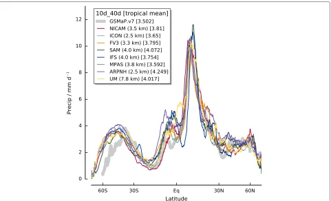
We start by comparing zonally and temporally averaged precipitation from the last 30 days of the DYAMOND simulations. This comparison is presented in Fig.5, which also includes precipitation estimated from observations for the same time period. The analysis by Kodama et al. (2012) identified a spin-up period of a few days in 14 km NICAM simulations. By discarding the initial 10 days, we thus avoid undue constraints from the initialization, as well as biases from differences in how the different mod-els spin-up. The comparison is nonetheless susceptible to a poor sampling of internal variability. To get a sense of the magnitude of the sampling error that may be associ-ated with this variability, we calculate the week-to-week standard deviation of the zonally averaged precipitation. It is about 15 % of the mean (or similar to the variabil-ity among the models) and does not vary systematically from model to model, or as a function of latitude. Being mindful of the sampling precision, Fig. 5 highlights the agreement among a large subset of the simulations in
terms of their representation of the zonally and globally averaged precipitation. Their tropical averaged precipi-tation for the final 30 days of the simulation is 3.813
± 0.164 mm d1 (1-sigma). ARPEGE-2.5 km simulates clearly larger precipitation (4.25 mm d1) as compared to the main group of models. This difference is believed to be the result of an artificial increase in surface evapora-tion which had been introduced into the lower resoluevapora-tion version of the model to improve its representation of tropical cyclone intensity, and for this reason, ARPEGE-2.5 km has been excluded from the subset. As discussed later, this also is believed to be responsible for ARPEGE-2.5 km producing much more intense tropical cyclones and also a much moister atmosphere, thus forming an interesting natural experiment. GEOS-3.3 km produces much less (3.2 mm d1) precipitation. This appears to be related to an output error, and a new set of simulations has been performed for inclusion in subsequent analy-sis. At the time of our analysis, however, this data was not available, so GEOS-3.3 km is not included in either the tabulation or the computation of the multi-model mean.
Compared to the cluster of models in Fig. 5, the observed precipitation (3.50 mm d1) for the same period—as estimated from calibrated microwave mea-surements to retrieve precipitation globally at 10 km spatial and hourly temporal scales—is at the two-sigma range of this group of models. The observations and models differ by an amount that is larger than the week-to-week variability just south of the Equator, where the simulations have a secondary peak in precipitation that is more pronounced than is observed, and in the very high latitudes of the Southern Hemisphere. The greater than observed precipitation just south of the Equator may represent a bias of the models, akin to the double ITCZ bias that is familiar from models of parameter-ized convection, or may be indicative of a deficiency in the observational retrievals in capturing what can often be intense precipitation from relatively isolated warm (congestus) clouds. Discrepancies at high latitudes are within the range of other observational products, e.g., the IMERGE product retrieves twice as much precipita-tion at 50◦S as compared to GSMaP.v7 (Hiro Masunaga, Yukari Takayabu, personal communication, 2018; GSMaP: Kubota et al. (2007)). Differences in the observed global mean and that simulated by the subset of models in Fig.5cannot however be explained by differences at high latitudes.
Fig. 5Mean precipitation. Precipitation is zonally and temporally averaged (over the last 30 days of the simulation) for each of the indicated models. The global averaged precipitation for each model is indicated in the legend. Mean precipitation from the GSMaP project (version 7) is provided as a reference. The GSMaP line width is to distinguish it from the models, not a measure of retrieval uncertainty
Table 6Tropical budgets
Model Pmm d1 PW mm I
thermalW m−2 IsolarW m−2
ARPEGE-NH 4.25 40.9 −265.4 319.3
FV3 3.80 38.7 −269.0 307.6
GEOS n/a 39.5 −269.2 303.1
ICON 3.65 38.8 −264.1 295.2
IFS 3.75 35.4 −268.4 312.2
MPAS 3.59 37.1 −265.9 327.3
NICAM 3.81 41.5 −259.2 327.0
SAM 4.07 37.3 −272.3 311.7
UM 4.02 38.1 −267.4 309.0
Observed 3.50 39.5 −259.6 306.4
Mean 3.81 38.3 −266.8 312.5
Stddev 0.16 1.7 2.5 10.4
Tropically (latitudes within 30◦of the Equator) averaged quantities related to the global hydrological cycle. For the observations, the GSMaP (v7) retrieval is used for precipitation,P; precipitable water, PW, is calculated only over the ocean for which observational estimates are taken from GMI. Top-of-atmosphere net solar,Isolar, and thermal infraredIthermalirradiances are taken from the CERES SYN1deg daily Terra and Aqua product. For precipitation and precipitable water, ARPEGE-NH is excluded from the calculation of the multi-model mean
couples most directly to the circulation. The column water burden is only calculated over the ocean, to better enable comparisons with observations. Compared to the obser-vations, the simulations appear somewhat less cloudy, as on average they are radiating thermal energy to space at a slightly greater rate than observed, but also absorb-ing a commensurately larger amount of solar energy. The net imbalance is quite close to observed, but differences among models can be large. NICAM-3.5 km simulates energy being absorbed at about twice the rate simulated by ICON (67.8 W m−2versus 31.1 W m−2). Such differences notwithstanding, given that this was the first time most of these models were ever run in such a configuration, and that no effort has been made to match the observations, we judge the degree of similitude with the observations as encouraging.
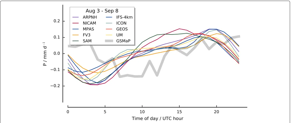
Globally, precipitation in the simulations peaks when the sun is in the western hemisphere, around 2000 UTC in most models, albeit somewhat earlier (nearer 1500 UTC) in SAM-4.3 km and NICAM-3.5 km. GSMaP (v7) pre-cipitation retrievals are noisier, but are also indicative of a 24-h cycle peaking when the sun is in the western hemisphere. As far as the minimum in precipitation is concerned, which according to retrievals occurs between 0700 and 1000 UTC, all models tend to show a sim-ilar feature somewhat earlier. Locally, over land, it is well known that convective precipitation tends to peak in the late afternoon or early evening, while over ocean the peak is more in the morning hours. The simulated and observed 24-h cycle thus reflects the inhomoge-neous distribution of precipitation zonally, where a peak near 2000 UTC would arise from the synchronization of precipitation maximizing over the warmer waters around the Maritime Continent (Warm Pool) with that over Africa. The slightly earlier peak in precipitation from NICAM-3.5 km and SAM-4.3 km may imply a greater contribution of precipitation from the monsoon regions of South Asia.
Predictability Tropical cyclones
Given the very large data volumes involved, for the pur-poses of this study, we identified tropical cyclones with the help of an algorithm that searched for contiguous and non-stationary tracks defined by a minimum in the surface pressure, over the ocean, equatorward of 30◦. Tracks lasting more than 1.5 days and with a mini-mum along track surface pressure less than 985 hPa were identified as tropical cyclones. The chosen threshold is slightly lower than that 994 hPa used to track cyclones in output from coarser resolution models (Roberts et al. 2015). For consistency across the models, the anal-ysis was performed on each model’s surface pressure fields after first being remapped to the standard 0.1◦ grid, masking land points using the CDO land-sea mask3, and with a 6-h time increment. To test this simple approach, it was compared to a more comprehensive algorithm (Kodama et al. 2015), based on the three-dimensional temperature and wind fields, applied to 30 years of data from a previous 14-km NICAM simula-tion. Application of the simple algorithm to the NICAM output resulted in an identification of nearly 90 % of the tropical cyclones identified by the more complex algorithm.
3Some outliers associated with persistent features with anomalously low
pressure (<840 hPa) were additionally filtered (mostly in the FV3 output), as these were believed to arise from cyclones interacting with land which were not filtered by the CDO land mask.
The algorithm was applied to the entire 40-day period for 8 simulations, resulting in the identification of 76 trop-ical cyclones, or just over 9 per simulation. The track of each tropical cyclone identified by the algorithm is shown in Fig.7. The median number of identified tropical cyclones was 8.5. As compared to the other simulations, GEOS-3.3 km output is an outlier, in that it identified twenty tropical cyclones. In reality, between 1 August and 10 September 2016, 14 tropical cyclones with Ps,min ≤
985 hPa formed—8 in the western North Pacific (WNP) and 3 each in the eastern North Pacific (ENP) and Atlantic. One deep depression, but no cyclones, formed in the Northern Indian Ocean during this period. When limiting the classification to stronger tropical cyclones
Ps,min ≤ 970 hPa, the models identified 3 to 7 (mean
of 4.9) tropical cyclones each4 (mean of 2.7 in WNP, 0.7 in Atlantic, 1.5 in ENP). In reality, six cyclones with
Ps,min≤970 hPa formed during this period, three
(Lion-rock, Namtheun, Meranti) in the WNP, two in the ENP, and one (Gaston) in the Atlantic. Among the simulations, ARPEGE-2.5 km produces unrealistically strong cyclones; five tropical cyclones had Ps,min ≤ 900 hPa, and the
tropical cyclone it formed in the Gulf of Mexico saw its pressure drop to 845 hPa; a value 25 hPa lower than the lowest ever recorded in a tropical cyclone. To explore this issue, an extra simulation of a few days was per-formed with ARPEGE-2.5 km using the corrected setting for the evaporation coefficient. This simulation leads to substantially less deepening and explains most, if not all, of the difference as compared to the other models. Given the obvious question marks (tropical cyclone strength in ARPEGE-2.5 km and number in GEOS), and keeping in mind limitations in the present approach to tracking, the similitude between the observations and the simu-lations is surprisingly large and encouraging of further research.
Integrated water vapor
In the tropics, precipitation and circulation are very tightly coupled, and column water is a very good indi-cator of precipitation (Bretherton et al. 2004; Peters and Neelin 2006; Mapes et al. 2018). These qualities, com-bined with sharp spatial gradients in the vicinity of pre-cipitation, identify column water vapor as an interesting quantity for prediction—something of a tropical analogue to the mid-troposphere geopotential field in the extra tropics. Using the DYAMOND models, we explore some aspects of the predictability of this (and other fields) for simulations in which the tropical dynamics are not dis-torted by the well-known deficiencies of parameterized convection. Similar questions have been explored before
Fig. 6Composite diurnal cycle of global precipitation as anomaly from mean
using a single model (e.g., Mapes et al. (2008), Brether-ton and Khairoutdinov (2015), Judt (2018)), and this is the first time that they have been explored using a real-istic surface orography and with an ensemble of different models.
Both Mapes et al. (2008) and Bretherton and Khairout-dinov (2015) measured error growth through the growth of (nearly) infinitesimal differences in precipitable water between pairs of otherwise identical runs. They showed that this measure of error growth saturates on small scales after about 2 to 4 days. At larger scales, and hence glob-ally, it saturates after 14 to 30 days. On no scale could these studies discern a difference between the tropics and extra-tropics. Judt (2018) did not address the differ-ence between tropical and extra-tropical error growth, but showed that—unlike for water vapor—the growth of perturbation energy increases relatively more rapidly at smaller scales, where the kinetic energy spectrum is relatively flatter (k−5/3).
The DYAMOND simulations are consistent with the earlier analysis, though a hint of extended predictability in the tropics merits further analysis. This conclusion is drawn from Fig. 8 which presents the zonally averaged anomaly column water vapor covariance between a pair of models (ICON-2.5 km and FV3-3.3 km) as a function of latitude. The covariance (normalized at each latitude by the mean variance of ICON at that latitude) decays with time—as expected from the chaotic dynamics of the atmo-sphere. After about 14 days, the covariance has decayed to near zero suggesting that the ability of one model to predict the other’s evolution has an envelope of about 2 weeks. This is indicative of somewhat less predictability
than found from the single model aqua-planet studies of previous investigators. The envelope of positive covari-ance (green colors) appears slightly more extended with time toward the Equator, suggesting that the chaotic dynamics may scramble signals in these regions somewhat less efficiently.
These questions are pursued more quantitatively by comparing the decay of the global mean covariance across pairs of models, and among perturbation experiments using slightly different configurations of a single model, in this case 2.5 km and two simulations with ICON-5 km. The latter is more akin to experiments analyzed in the earlier literature and as discussed above. This analy-sis, Fig.9, confirms the impression of a roughly 2-week envelope of coherence across the models. Simulations with slight perturbations in the configuration of ICON, however, show longer coherence, suggesting an intrinsic predictability limit approaching 3 weeks—more consis-tent with earlier studies. The slight pick up of covariability after about 5 weeks may be due to the seasonal cycle or a signature of intraseasonal variability. The additional data from the accidental ensemble offers additional opportuni-ties to explore these issues. Looking across the simulations to identify if particular features (like envelopes of tropical cyclone genesis, or breaks in the monsoon) are predictable with longer lead times might help to identify additional sources of predictability, as discussed by Fudeyasu et al. (2008) among others.
Summary and outlook
Fig. 7Tropical cyclone tracks. Tracks of tropical cyclones identified from a subset of the available DYAMOND models following procedures outlined in the text. Total number of tropical cyclones identified given in parentheses
had been well demonstrated (e.g., Tomita et al. (2005), Satoh et al. (2008)). The simulations described here, performed by nine different groups from six national entities across three continents, demonstrate that such simulations have now gone from being feasible to practical.
With the increasing practicality of such simulations, it becomes possible to begin answering some basic ques-tions. For instance, how sensitive are the simulations to a particular implementation? Before DYAMOND, most of the global storm-resolving models used here had never been run in this configuration, and no two models had ever before attempted to perform the same simulations. Based on our preliminary analysis, we find that basic aspects of the general circulation are well captured by the storm-resolving models. The outgoing long-wave radia-tion is well simulated, as is the global precipitaradia-tion and distribution of precipitable water. Agreement among the models is such that it is difficult to establish if differences with observations—for instance, more precipitation in the poleward flank of the storm tracks and in the equatorial region just south of the Equator—represent deficiencies in the models or in the retrievals of these quantities. The visual representation of clouds is, from a geosta-tionary field of view, practically indistinguishable from observations. Insofar as it can be determined given the brevity of the simulations and the basic storm-tracking algorithm, the tropical genesis and intensification statis-tics of tropical cyclones are well captured. About the right number of tropical cyclones form in about the right place and intensify in about the right proportion. Despite its very different dynamics, the simulations suggest that predictability time scales in the tropics are similar, or perhaps even slightly longer, than in the mid-latitudes. Finally, we identify a diurnal cycle in global precipita-tion that is consistent across all simulaprecipita-tions and similarly evident in the observations. Considering that the mod-els were not specifically tuned for this case and that minor implementation errors are to be expected given the early stage of the development, this agreement is remarkable.
The simulations are not without their deficiencies. Even the present, relatively superficial, analysis makes
clear that to reap the rewards of being able to simu-late the general circulation of Earth’s global atmosphere at storm-resolving scales, some unconstrained degrees of freedom remain to be tamed. Our preliminary analysis identifies challenges in linking energy and water budgets, as evidenced by differences in shortwave (solar) irradi-ances at top-of-atmosphere, a quantity that is likely to be influenced by the representation of (often shallow) clouds, turbulence, and cloud microphysical processes. However, by virtue of the ability of GSRMs to directly link these processes to the circulation on the one hand, and observations at similar scales on the other, we are optimistic that research targeted at addressing these chal-lenges will bear fruit. If so, GSRMs will provide an improved physical foundation for model-based investiga-tions of Earth’s climate and climate change and usher in a new generation of climate models. With their ability to explicitly resolve convective storms, GSRMs may also transform the weather prediction enterprise and lead to improved forecasts of severe weather from local to global scales.
Fig. 8Water vapor anomaly correlation. Zonally averaged anomaly correlation of hourly (0.1 degree) precipitable water between ICON-2.5 km and GEOS-3.3 km normalized by zonally and temporally averaged water vapor variance from ICON-2.5 km plotted as a function of time and latitude
domain-specific analysis tools. Use of compressed data formats greatly reduced the data volumes, but was subject to the dynamic range of the data, which in some cases was artificially inflated by inadequate filtering of insignificant values.
Any attempt to give a comprehensive overview of mod-els that contain such a fantastic range of scales for a fluid whose dynamics are as diverse and heterogeneous as Earth’s atmosphere will be necessarily superficial. Our hope is that by documenting the DYAMOND simulations,
curating subsets of their output, and by making this, as well as their full output, available for analysis by the broader research community, a more specific, and thereby in-depth, analysis will follow. Toward this end, we have also used this manuscript to highlight differences in model formulation which makes their comparison interesting, as well as features of the simulations that we noticed and believe merit further study. To organize the dissemination of findings from studies of these and related questions, a subset of the present authors have also organized a
special issue of theJournal of the Meteorological Society of Japan5. We hope that it will also help nucleate inter-est into a new generation of models that many of us believe offers the best, and perhaps only, chance to resolve long-standing biases in conventional representations of the climate system.
Abbreviations
DKRZ: German Climate Computing Center; ECMWF: European Centre for Medium-range Weather Forecasts; GEOS: Goddard Earth Observing System; GSRM: Global storm-resolving Model; ICON: Icosahedral non-hydrostatic model; IFS: Integrated Forecast System of the ECMWF; MPAS: Model for Predicting Across Scales; NICAM: Non-hydrostatic Icosahedral Atmospheric Model; SAM: Global System for Atmospheric Modeling; UM: Unified model of the United Kingdom’s Meteorological Service
Acknowledgements
BS thanks the AORI at the University of Tokyo who supported an extended visit to the University of Tokyo which facilitated the writing of this manuscript. Prof. Yukari Takayabu is thanked for her input on and provision of the GSMaPv6 precipitation retrievals. The NICAM simulations were performed on the Earth Simulator at the Japan Agency for Marine-Earth Science and Technology (JAMSTEC). Peter Caldwell is thanked for constructive comments on an earlier draft.
Authors’ contributions
MS and BS conceived of the project, and together with JB and CSB designed the study. LA, XC, PD, FJ, DK, LK, MK, WP, JLS, RS, BV, PLV, NW, and LZ performed or contributed to the simulations described in the manuscript. NR provided the scientific visualization and drafted Figs. 1–4. PN developed and lead the data infrastructure and performance review of the models. DK, BS, and CK performed the analysis. BS wrote the manuscript incorporating input from all authors. All authors read and approved the final manuscript.
Funding
This work was supported by the Max Planck Society, the European Union’s Horizon 2020 research and innovation program under grant agreement ESiWACE No 675191, and the High-Definition Clouds and Precipitation for Climate Prediction (HD(CP)2)project of the German Ministry for Education and
Research (BMBF) within the framework program “Research for Sustainable Development (FONA)”, www.fona.de, under the number FKZ: 01LK1211A/C. MS, CK, and RS are supported by the FLAGSHIP2020 within the priority study4 (Advancement of meteorological and global environmental predictions utilizing observational “Big Data”) and the “Integrated Research Program for Advancing Climate Models (TOUGOU program)” from the Ministry of Education, Culture, Sports, Science and Technology (MEXT), Japan. Marat Khairoutdinov was supported by the NSF Grant AGS1418309 to Stony Brook University, and also by the NCAR-Wyoming Supercomputing Center, where SAM simulation was performed.
Availability of data and materials
Model output supporting the conclusions of this article are archived by the German Climate Computing Centre (DKRZ) and made available through the ESiWACE project (https://www.esiwace.eu/services/dyamond).
Competing interests
The authors declare that they have no competing interest.
Author details
1Max Planck Institute for Meteorology, Bundesstraße 53, 20146, Hamburg,
Germany.2Atmosphere and Ocean Research Institute, The University of Tokyo, 5-1-5 Kashiwanoha, Kashiwa, Chiba, 277-8564, Japan.3CNRM Météo-France, 42
av. G. Coriolis, 31057 Toulouse Cedex 1, France.4German Climate Computing Center, DKRZ, Bundesstrasse 45a, 20146, Hamburg, Germany.5Department of
Atmospheric Sciences, University of Washington, Box 351640, Seattle, WA, 98195-1640, USA.6Geophysical Fluid Dynamics Laboratory, Princeton
University, Forrestal Campus/U.S. Route 1, P.O. Box 308, Princeton, NJ, 08542, USA.7ECMWF, Shinfield Road, Reading, RG2 9AX, UK.8National Center for
5https://jmsj.metsoc.jp/CallForPaper_2019JMSJ_DYAMOND.pdf
Atmospheric Research, PO Box 3000, Boulder, CO, 80303-3000, USA.9School of
Marine and Atmospheric Sciences, Stony Brook University, Stony Brook, NY, 11794-5000, USA.10Hans-Ertel-Zentrum für Wetterforschung, Deutscher
Wetterdienst, Frankfurterstrasse 135, Offenbach, Germany.11Japan Agency for
Marine-Earth Science and Technology, 3173-15, Showa-machi, Kanazawa-ku, Yokohama, Kanagawa, 236-0001, Japan.12NASA Global Modeling and
Assimilation Office, Goddard Space Flight Center, Greenbelt, Maryland, USA.
13National Centre for Atmospheric Science, University of Reading, Reading, UK.
Received: 2 March 2019 Accepted: 28 July 2019
References
Bessho K, Date K, Hayashi M, Ikeda A, Imai T, Inoue H, Kumagai Y, Miyakawa T, Murata H, Ohno T, Okuyama A, Oyama R, Sasaki Y, Shimazu Y, Shimoji K, Sumida Y, Suzuki M, Taniguchi H, Tsuchiyama H, Uesawa D, Yokota H, Yoshida R (2016) An introduction to Himawari-8/9 –Japan’s
new-generation geostationary meteorological satellites. J Meteorol Soc Jpn 94(2):151–183.https://doi.org/10.2151/jmsj.2016-009
Bethel EW, Childs H, Hansen C (2012) High performance visualization: enabling extreme-scale scientific insight. Chapman & Hall/CRC, New York.https:// doi.org/10.1201/b12985
Bony S, Stevens B, Frierson DMW, Jakob C, Kageyama M, Pincus R, Shepherd TG, Sherwood SC, Siebesma AP, Sobel AH, Watanabe M, Webb MJ (2015) Clouds, circulation and climate sensitivity. Nat Geosci 8(4):261–268 Bretherton CS, Peters ME, Back LE (2004) Relationships between water vapor
path and precipitation over the tropical oceans. J Clim 17(7):1517–1528 Bretherton CS, Khairoutdinov MF (2015) Convective self-aggregation
feedbacks in near-global cloud-resolving simulations of an aquaplanet. J Adv Model Earth Syst 7(4):1765–1787
Bubnová R, Hello G, Bénard P, Geleyn J-F (1995) Integration of the fully elastic equations cast in the hydrostatic pressure terrain-following coordinate in the framework of the arpege/aladin nwp system. Mon Weather Rev 123(2):515–535
Clyne J, Mininni P, Norton A, Rast M (2007) Interactive desktop analysis of high resolution simulations: application to turbulent plume dynamics and current sheet formation. New J Phys 9(8):301
Cotton WR, Tripoli GJ (1978) Cumulus convection in shear flow—three-dimensional numerical experiments. J Atmos Sci 35(8):1503–1521
Fudeyasu H, Wang Y, Satoh M, Nasuno T, Miura H, Yanase W (2008) Global cloud-system-resolving model NICAM successfully simulated the lifecycles of two real tropical cyclones. Geophys Res Lett 35(22):2397–6
Hohenegger C, Kornblueh L, Becker T, Cioni G, Engels JF, Klocke D, Schulzweida U, Stevens B (2019) Convergence of zero order climate statistics in global simulations using explicit convection. J Meteorol Soc Jpn
Ito J, Hayashi S, Hashimoto A, Ohtake H, Uno F, Yoshimura H, Kato T, Yamada Y (2017) Stalled improvement in a numerical weather prediction model as horizontal resolution increases to the sub-kilometer scale. SOLA 13(0):151–156
Jubair MI, Alim U, Röber N, Clyne J, Mahdavi-Amiri A (2016) Icosahedral maps for a multiresolution representation of earth data. In: VMV ’16 Proceedings of the Conference on Vision, Modeling and Visualization, Bayreuth. pp 161-168
Judt F (2018) Insights into atmospheric predictability through global convection-permitting model simulations. J Atmos Sci 75(5):1477–1497 Khairoutdinov MF, Randall DA (2003) Cloud resolving modeling of the ARM
summer 1997 IOP: model formulation, results, uncertainties, and sensitivities. J Atmos Sci 60(4):607–625
Klemp JB, Wilhelmson RB (1978) The simulation of three-dimensional convective storm dynamics. J Atmos Sci 35(6):1070–1096 Klocke D, Brueck M, Hohenegger C, Stevens B (2017) Rediscovery of the
doldrums in storm-resolving simulations over the tropical Atlantic. Nat Geosci 183(4):153–7
Kodama C, Noda AT, Satoh M (2012) An assessment of the cloud signals simulated by NICAM using ISCCP, CALIPSO, and CloudSat satellite simulators. J Geophys Res-Atmos 117(D12):1–17
Kubota T, Shige S, Hashizume H, Aonashi K, Takahashi N, Seto S, Hirose M, Takayabu YN, Ushio T, Nakagawa K, Iwanami K, Kachi M, Okamoto K (2007) Global precipitation map using satellite-borne microwave radiometers by the gsmap project: production and validation. IEEE Trans Geosci Remote Sens 45(7):2259–2275.https://doi.org/10.1109/TGRS.2007.895337 Langhans W, Schmidli J, Schär C (2012) Bulk convergence of cloud-resolving
simulations of moist convection over complex terrain. J Atmos Sci 69(7):2207–2228
Lin S-J, Rood RB (2004) A “vertically Lagrangian” finite-volume dynamical core for global models. Mon Weather Rev 132(544):2293–307
Malardel S, Wedi N, Deconinck W, Diamantakis M, Kuehnlein C, Mozdzynski G, Hamrud M, Smolarkiewicz P (2016) A new grid for the IFS. ECMWF Newsl 146:23–28.https://doi.org/doi:10.21957/zwdu9u5i
Mapes B, Tulich S, Nasuno T, Satoh M (2008) Predictability aspects of global aqua-planet simulations with explicit convection. J Meteorol Soc Jpn Ser II 86A:175–185
Mapes BE, Chung ES, Hannah WM, Masunaga H, Wimmers AJ, Velden CS (2018) The meandering margin of the meteorological moist tropics. Geophys Res Lett 45(2):1177–1184
Marotzke J, Jakob C, Bony S, Dirmeyer PA, O’Gorman PA, Hawkins E, Perkins-Kirkpatrick S, Le Quere C, Nowicki S, Paulavets K, Seneviratne SI, Stevens B, Tuma M (2017) Climate research must sharpen its view. Nat Clim Chang 7(2):89–91
Matsuno T (2016) Prologue: tropical meteorology 1960–2010—personal recollections. Meteorol Monogr 56.https://journals.ametsoc.org/doi/pdf/ 10.1175/AMSMONOGRAPHS-D-15-0012.1 https://doi.org/10.1175/ AMSMONOGRAPHS-D-15-0012.1
Mengaldo G, Wyszogrodzki A, Diamantakis M, Lock S-J, Giraldo FX, Wedi NP (2018) Current and emerging time-integration strategies in global numerical weather and climate prediction. Arch Comput Methods Eng:1–22.https://doi.org/10.1007/s11831-018-9261-8
Neumann P, Dueben P, Adamidis P, Bauer P, Brueck M, Kornblueh L, Klocke D, Stevens B, Wedi N, Biercamp J (2019) Assessing the scales in numerical weather and climate predictions: will exascale be the rescue? Phil Trans R Soc 377:20180148.https://doi.org/10.1098/rsta.2018.0148
Palmer TN (2016) A personal perspective on modelling the climate system. Proc R Soc A 472(2188):20150772–14
Peters O, Neelin JD (2006) Critical phenomena in atmospheric precipitation. Nat Phys 2(6):393–396
Phillips NA (1956) The general circulation of the atmosphere: a numerical experiment. QJR Meteorol Soc 82(352):123–164
Putman WM, Lin S-J (2007) Finite-volume transport on various cubed-sphere grids. J Comput Phys 227(1):55–78
Putman WM, Suarez M (2011) Cloud-system resolving simulations with the NASA Goddard Earth Observing System global atmospheric model (GEOS-5). Geophys Res Lett 38(16)
Randall D, Khairoutdinov M, Arakawa A, Grabowski W (2003) Breaking the cloud parameterization deadlock. Bull Am Meteorol Soc 84(11):1547–1564 Roberts MJ, Vidale PL, Mizielinski MS, Demory M-E, Schiemann R, Strachan J,
Hodges K, Bell R, Camp J (2015) Tropical cyclones in the UPSCALE ensemble of high-resolution global climate models*. J Clim 28(2):574–596 Rodwell MJ, Palmer TN (2007) Using numerical weather prediction to assess
climate models 133(622):129–146
Saito K, Ishida J-I, Aranami K, Hara T, Segawa T, Narita M, Honda Y (2007) Nonhydrostatic Atmospheric Models and Operational Development at JMA. J Meteorol Soc Jpn Ser II 85B:271–304
Satoh M, Tomita H, Miura H, Iga S, Nasuno T (2005) Development of a global cloud resolving model - a multi-scale structure of tropical convections -. J Earth Simul 3:11–19
Satoh M, Matsuno T, Tomita H, Miura H, Nasuno T, Iga S (2008) Nonhydrostatic icosahedral atmospheric model (NICAM) for global cloud resolving simulations. J Comput Phys 227(7):3486–3514
Satoh M, Tomita H, Yashiro H, Miura H, Kodama C, Seiki T, Noda AT, Yamada Y, Goto D, Sawada M, Miyoshi T, Niwa Y, Hara M, Ohno T, Iga S-i, Arakawa T, Inoue T, Kubokawa H (2014) The Non-hydrostatic Icosahedral Atmospheric Model: description and development. Prog Earth Planet Sci 1:18.https:// doi.org/10.1186/s40645-014-0018-1
Satoh M, Tomita H, Yashiro H, Kajikawa Y, Miyamoto Y, Yamaura T, Miyakawa T, Nakano M, Kodama C, Noda AT, Nasuno T, Yamada Y, Fukutomi Y (2017) Outcomes and challenges of global high-resolution non-hydrostatic
atmospheric simulations using the K computer. Prog Earth Planet Sci 4:13. https://doi.org/10.1186/s40645-017-0127-8
Satoh M, Noda AT, Seiki T, Chen Y-W, Kodama C, Yamada Y, Kuba N, Sato Y (2018) Toward reduction of the uncertainties in climate sensitivity due to cloud processes using a global non-hydrostatic atmospheric model. Prog Earth Planet Sci 5:67.https://doi.org/10.1186/s40645-018-0226-1 Satoh M, Stevens B, JUdt F, Khairoutdinov M, Lin S-J, Putman WM, Düben P
(2019) Global cloud resolving models. Curr Clim Change Rep.https://doi. org/10.1007/s40641-019-00131-0
Skamarock WC, Klemp JB, Duda MG, Fowler LD, Park S-H, Ringler TD (2012) A Multiscale Nonhydrostatic Atmospheric Model Using Centroidal Voronoi Tesselations and C-Grid Staggering. Mon Weather Rev 140(9):3090–3105 Skamarock WC, Park S-H, Klemp JB, Snyder C (2014) Atmospheric Kinetic
Energy Spectra from Global High-Resolution Nonhydrostatic Simulations. J Atmos Sci 71(11):4369–4381
Smagorinsky J (1963) General circulation experiments with the primitive equations. Mon Weather Rev 91(3):99–164
Stevens B, Bony S (2013) What Are Climate Models Missing? Science 340(6136):1053–1054
Stevens B, Ament F, Bony S, Crewell S, Ewald F, Gross S, Hansen A, Hirsch L, Jacob M, Kölling T, Zinner T, Mayer B, Wendisch M, Wolf K, Ehrlich A, Farrell D, Forde M, Jansen F, Konow H, Wing AA, Klingebiel M, Wirth M, Brueck HM, Bauer-Pfundstein M, Delanoë J, Rapp M, Rapp AD, Hagen M, Peters G, Bakan S, Klepp C (2019) A high-altitude long-range aircraft configured as a cloud observatory– the NARVAL expeditions. Bull Amer Meteorol Soc Tomita H, Tsugawa M, Satoh M, Goto K (2001) Shallow Water Model on a
Modified Icosahedral Geodesic Grid by Using Spring Dynamics. J Comput Phys 174(2):579–613
Tomita H, Satoh M (2004) A new dynamical framework of nonhydrostatic global model using the icosahedral grid. Fluid Dyn Res 34(6):357–400. https://doi.org/10.1016/j.fluiddyn.2004.03.003
Tomita H, Miura H, Iga S, Nasuno T, Satoh M (2005) A global cloud-resolving simulation: Preliminary results from an aqua planet experiment. Geophys Res Lett 32(8):3283
Voldoire A, Decharme B, Pianezze J, Lebeaupin Brossier C, Sevault F, Seyfried L, Garnier V, Bielli S, Valcke S, Alias A, et al. (2017) Surfex v8.0 interface with oasis3-mct to couple atmosphere with hydrology, ocean, waves and sea-ice models, from coastal to global scales. Geosci Model Dev 10(11):4207–4227
Walters D, Baran A, Boutle I, Brooks M, Earnshaw P, Edwards J, Furtado K, Hill P, Lock A, Manners J, Morcrette C, Mulcahy J, Sanchez C, Smith C, Stratton R, Tennant W, Tomassini L, Van Weverberg K, Vosper S, Willett M, Browse J, Bushell A, Dalvi M, Essery R, Gedney N, Hardiman S, Johnson B, Johnson C, Jones A, Mann G, Milton S, Rumbold H, Sellar A, Ujiie M, Whitall M, Williams K, Zerroukat M (2017) The Met Office Unified Model Global Atmosphere 7.0/7.1 and JULES Global Land 7.0 configurations. Geosci Model Dev Discuss 2017:1–78
Wedi NP (2014) Increasing horizontal resolution in numerical weather prediction and climate simulations: illusion or panacea? Philos Trans R Soc A Math Phys Eng Sci 372(2018):20130289–20130289
Weisman ML, Skamarock WC, Klemp JB (1997) The Resolution Dependence of Explicitly Modeled Convective Systems. Mon Weather Rev 125(4):527–548 Williamson DL (2005) Moisture and temperature balances at the Atmospheric Radiation Measurement Southern Great Plains Site in forecasts with the Community Atmosphere Model (CAM2). J Geophys Res-Atmos 110(D15):3123–17
Williamson DL (2007) The Evolution of Dynamical Cores for Global Atmospheric Models. J Meteorol Soc Jpn Ser II 85B:241–269
Williams KD, Bodas-Salcedo A, Déqué M, Fermepin S, Medeiros B, Watanabe M, Jakob C, Klein SA, Senior CA, Williamson DL (2013) The Transpose-AMIP II Experiment and Its Application to the Understanding of Southern Ocean Cloud Biases in Climate Models. J Clim 26(10):3258–3274
Wood N, Staniforth A, White A, Allen T, Diamantakis M, Gross M, Melvin T, Smith C, Vosper S, Zerroukat M, Thuburn J (2013) An inherently mass-conserving semi-implicit semi-Lagrangian discretization of the deep-atmosphere global non-hydrostatic equations. QJR Meteorol Soc 140(682):1505–1520 Zängl G, Reinert D, Rípodas P, Baldauf M (2014) The ICON (ICOsahedral
Non-hydrostatic) modelling framework of DWD and MPI-M: Description of the non-hydrostatic dynamical core. QJR Meteorol Soc 141(687):563–579
Publisher’s Note