R E V I E W
Open Access
A review on the numerical simulation of
equatorial plasma bubbles toward scintillation
evaluation and forecasting
Tatsuhiro Yokoyama
Abstract
Equatorial plasma bubbles (EPBs) have been a longstanding and increasingly important subject because they cause severe scintillations in radio waves from Global Navigation Satellite System satellites. The phenomenon was found in the 1930s as irregular ionosonde observations and was termed equatorial spreadF(ESF). ESF is interpreted as plasma density irregularities associated with EPBs that have nonlinearly evolved into the topside ionosphere. Numerical simulations have been powerful tools to study the fully nonlinear evolution of EPBs, which cannot be wholly
understood from theoretical predictions. In this paper, historical achievements in the numerical simulation of EPBs are reviewed, and future directions toward scintillation evaluation and forecast are discussed.
Keywords: Equatorial ionosphere, Equatorial spreadF, Equatorial plasma bubbles, Numerical simulation, Scintillation, High-performance computing, Space weather
Introduction
Satellite communication and navigation are often dis-rupted by irregularities in the ionospheric plasma den-sity. Fresnel scale irregularities cause rapid fluctuations in the signal phase and amplitude, a phenomenon known as ionospheric scintillation (e.g., Yeh and Liu 1982; Kintner et al. 2007 and references therein). Under the phase screen approximation, the Fresnel scale is given by √
2λz, whereλis the radio wavelength andzis the height of the irregularity layer (Kintner et al. 2007). Under the assumption that plasma density irregularities exist in the ionosphericFregion, the Fresnel scale for the L-band fre-quencies used in the Global Navigation Satellite System (GNSS) is 300–400 m. The evaluation and forecast of such plasma density irregularities are now regarded as a critical issue for stable communication and precise navigation.
Severe ionospheric scintillations in the equatorial ionosphere are caused by a phenomenon called equatorial spreadF(ESF) or equatorial plasma bubbles (EPBs) (e.g., Hysell 2000; Woodman 2009). Although the Rayleigh– Taylor instability has been considered as a likely candidate
Correspondence: [email protected]
National Institute of Information and Communications Technology, 4-2-1 Nukui-Kitamachi, Koganei, Tokyo 184-8795, Japan
for ESF generation, it cannot explain the irregularities in the topsideFregion, where linear theory predicts plasma irregularities should be stabilized (e.g., Dungey 1956; Farley et al. 1970). Woodman and LaHoz (1976) pro-posed the concept of ionospheric “bubbles,” which non-linearly evolve from the bottomside and penetrate above the F peak altitude. EPBs contain a broad spectrum of plasma density irregularities, as measured by sound-ing rockets and satellites. Plasma density undulations with wavelengths of hundreds of kilometers have often been observed before the onset of EPB formation and have recently been termed large-scale wave structures (Tsunoda and White 1981; Tsunoda 2015). Intermediate-and short-scale irregularities (tens of kilometers to the sub-meter scale) have been found to be dominant in fully developed EPBs with multiple spectral indices (e.g., Rino et al. 1981; Singh and Szuszczewicz 1984; Carrano and Rino 2016). Such spectral characteristics are analogous but not identical to neutral turbulence (Kelley and Hysell 1991). To evaluate scintillation effects, intermediate-scale irregularities must be resolved in numerical models.
The first numerical simulation to study EPBs was conducted by Scannapieco and Ossakow (1976), who successfully reproduced a low-density region pen-etrating nonlinearly through the topside F region.
Since then, a number of numerical simulations of the nonlinear evolution of EPBs have been conducted, as reviewed in the following sections. The most recent models developed by the author and colleagues could reproduce very turbulent structures inside EPBs (Yokoyama et al. 2014, 2015; Yokoyama and Stolle 2017; Rino et al. 2017). The purpose of this article is to review the development of numerical simulations of EPBs over the past 40 years and discuss a possible future research direction involving the use of state-of-the-art numerical models toward the evaluation and forecast of ionospheric scintillations.
Theory
Although each numerical model solves each set of equations with different parameters and numerical schemes, they are governed by the fundamental laws of ionospheric electrodynamics: the continuity and steady-state momentum equations for ions and electrons and the divergence-free current condition (see also Kelley 2009; Yokoyama and Stolle 2017). Under the simplifying assumption of a single ion species, these equations are written as
∂Ni
∂t + ∇ ·(NiVi)=Si (1)
e(E+Vi×B)+Mig−∇(Ni
kBTi)
Ni +
Miνin(U−Vi)=0
(2)
−e(E+Ve×B)+Meg−∇(
NekBTe)
Ne +
Meνen(U−Ve)=0
(3)
∇ ·J= ∇ ·[e(NiVi−NeVe)]=0, (4) whereNi,eis the ion/electron density (Ni=Ne=Nunder the quasi-neutrality condition), Vi,e is the ion/electron velocity, Si represents the chemical terms, e is the ele-mentary charge,E = E0− ∇φ is the electric field,E0is
the background electric field,φ is the electrostatic polar-ization potential, Bis the geomagnetic field, Mi,e is the ion/electron mass,gis the acceleration due to gravity,kB is the Boltzmann constant, Ti,e is the ion/electron tem-perature,νin,enis the ion/electron collision frequency with neutrals,Uis the neutral wind velocity, andJis the total current density.
For simplicity, the neutral wind velocity U was set to zero, and the appropriate approximation for the equato-rialFregion was applied. The ion and electron velocities and the current densityJare then given by
Vi=
Miνin
eB2 E+E×B/B 2+ Mi
eB2g×B− kBTi
eNB2∇N×B (5)
Ve=E×B/B2+
kBTe
eNB2∇N×B (6)
J=eN(Vi−Ve)=σPE+
NMi
B2 g×B−
kB(Ti+Te)
B2 ∇N×B,
(7)
whereσP ≈NMiνin/B2is the Pedersen conductivity. The linear growth rate of the Rayleigh–Taylor instability is obtained by substituting Eqs. (5) and (7) into Eqs. (1) and (4) for the linear analysis. The pressure-gradient-driven current (the third term of Eq. (7)), which produces a dia-magnetic current and enhances the main dia-magnetic field intensity inside the EPBs (Stolle et al. 2006; Aveiro et al. 2011; Yokoyama and Stolle 2017) vanishes in Eq. (4), and thus, the Pedersen and gravity-driven currents are the major drivers of the instability. In the presence of a zeroth-order vertical (z-directional) density gradient, the linear growth rate is derived as
γ = νg in
1
N ∂N
∂z. (8)
The growth rate is positive when the density gradient is antiparallel tog. Therefore, the linear theory predicts unstable conditions only below the F peak altitude, but density irregularities appear throughout the F region. The nonlinear terms in Eqs. (1) and (4) should be taken into account to understand the fundamental mechanisms behind the development of EPBs, for which numerical simulations have been developed since the late 1970s.
Numerical schemes
of the flow. The flux-corrected transport (FCT) method (Zalesak 1979) has been a popular scheme in the iono-spheric modeling field (e.g., Zalesak and Ossakow 1980; Retterer 2010a). The FCT scheme implements a flux lim-iter by combining higher and lower order schemes so as not to produce overshoot or undershoot at the subsequent time step. A similar technique called the partial donor cell method (Hain 1987) has been applied to recent mod-els (e.g., Huba and Joyce 2007; Huba et al. 2008). The total variation diminishing (TVD) method (Harten 1983) is another popular technique that can capture shock-like structures without oscillation (e.g., Aveiro and Hysell 2010; Hysell et al. 2014b). Among these advanced algo-rithms, in the authors’ experience (e.g., Yokoyama et al. 2014), the constrained interpolation profile (CIP) method (Yabe et al. 2001, 2004) is the best method to deal with ionospheric irregularities. The CIP method treats the first-order spatial derivatives of the plasma density as dependent variables so that plasma density gradients are transported over time. With the third-order accu-racy maintained in time and space, shock-like EPB walls and turbulent internal structures can be captured by the CIP method.
Equation (4) can be rewritten as
∇ ·(· ∇φ)=S(g,E0,U), (9)
which is a boundary value problem for the electrostatic potential φ with the source function S and yields a sparse linear system of equations. Classical direct meth-ods, such as Gaussian elimination, can be used to solve this problem within a finite number of operations; how-ever, such methods destroy the sparsity of the matrix and necessitate the allocation of a huge amount of additional memory. An efficient direct solver called the stabilized error vector propagation (SEVP) method (Madala 1978) has been applied in recent models (e.g., Retterer 2010a; Duly et al. 2014). Generally, iterative methods are pre-ferred for sparse linear system solvers because the sparse matrix–vector product is the main operation during each iteration. However, classical iterative solvers, such as the Jacobi, Gauss–Seidel, and successive over-relaxation (SOR) methods, do not converge effectively in large-scale three-dimensional (3D) problems. As an alternative, Krylov subspace methods have been developed as effec-tive sparse linear system solvers. Examples of the variants of the Krylov subspace methods include the conjugate gra-dient (CG), biconjugate gragra-dient stabilized (BiCGSTAB), and generalized minimum residual (GMRES) methods. In combination with appropriate preconditioning tech-niques such as incomplete LU factorization on paral-lel computers, Krylov subspace methods can achieve excellent convergence efficiency. A different approach called the multigrid method exploits discretizations with a hierarchy of grid coarseness levels to obtain optimal
convergence using relaxation techniques. Saad (2003) has provided a detailed explanation of iterative methods, including a theoretical background and different types of algorithms used in such methods. A new algorithm of the Krylov subspace method is currently under devel-opment (e.g., Fujino and Murakami 2013) and has been implemented in new simulation models (e.g., Yokoyama et al. 2014). Some software packages of sparse linear system solvers are available online, including SPARSKIT (http://www-users.cs.umn.edu/ saad/software/SPARSKIT) (Saad 1990) and MUDPACK (https://www2.cisl.ucar.edu/ resources/legacy/mudpack) (Adams 1991).
Two-dimensional models
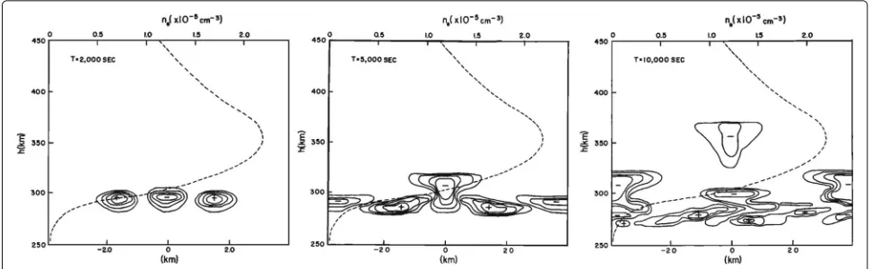
As mentioned above, the linear theory of the Rayleigh– Taylor instability does not predict the appearance of ESF above theFpeak altitude, where the plasma density gra-dient has the same orientation as the gravitational force. It is essential to understand the nonlinear behavior of equatorial ionospheric plasma instabilities, which can be realized only through numerical simulation. Fortunately, the geometry of the equatorial ionosphere can be simpli-fied easily on a two-dimensional (2D) plane. When the zonal and vertical directions are defined as the two axes of the simulation domain at the dip equator, the geomagnetic field is perpendicular to the plane, allowing the electro-dynamics parallel to the geomagnetic field to be ignored. Figure 1 shows the results obtained by Scannapieco and Ossakow (1976). Although the simulated EPB structure was oversimplified and took a very long time to evolve to the topside, it was an important achievement to simu-late the penetration of the density irregularities generated in the bottomside F region into the topside F region, where the linear theory predicts no irregularities to exist.
Fig. 1The first 2D simulation of the nonlinear evolution of EPBs. Reproduced from Scannapieco and Ossakow (1976)
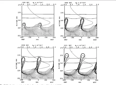
in Fig. 3. Even though the neutral wind was uniform in altitude, the zonal drift velocity driven by the F-region dynamo tended to have a vertical shear as a function ofPF/PF+PE, wherePF andPE are the flux-tube-integrated Pedersen conductivities in the F and E regions, respectively. An important implication of this result is that
the variations of physical parameters along geomagnetic field lines should be taken into account, which has led to the progress of theoretical work (e.g., Sultan 1996) and 3D numerical models, as presented in the next section.
Once the instability is triggered and irregularities have formed inside EPBs, they may cause severe scintillations.
Fig. 3EPBs tilted by neutral wind effects. Reproduced from Zalesak et al. (1982)
The degree to which satellite signals are affected by the irregularities depends on the spectral characteris-tics of the irregularities. Although the important fea-tures of large-scale EPBs observed at that time were clearly reproduced by Zalesak et al. (1982), intermediate-scale structures close to the Fresnel intermediate-scale of VHF and L-band signals were also studied through simu-lations and compared with in situ observations (e.g., Keskinen et al. 1981; Zargham and Seyler 1987, 1989; Kelley et al. 1987). Because it was not easy to capture a wide range of irregularity spectra using simulation mod-els at that time, these modmod-els have limited spatial domains and focused on only intermediate-scale irregularities. A recent high-resolution model may be able to consider unified spectral characteristics along with large-scale non-linear EPB formation (Rino et al. 2017).
A longstanding and still unresolved problem in the equatorial ionosphere is what triggers ESF/EPBs. Day-to-day variability in the occurrence of ESF is largely unpre-dictable (e.g., Hysell and Burcham 2002; Woodman 2009; Retterer and Roddy 2014). Because the linear growth rate of the Rayleigh–Taylor instability on its own cannot be
large enough to account for the rapid growth of EPBs from thermal fluctuations (e.g., Farley et al. 1970), an initial “seeding” is required in EPB simulations. In most previ-ous simulations, plasma density perturbations have been used as the initial seeding, but the source of such ini-tial density perturbations has not been discussed. Mean-while, the interaction between atmospheric gravity waves (AGWs) and ionospheric plasma has long been consid-ered as a plausible mechanism to modulate the ionosphere (Hines 1960). From Jicamarca radar observations, Kelley et al. (1981) have proposed that the modulation of the bottomside density gradient induced by AGWs is ampli-fied by the Rayleigh–Taylor instability. The seeding effect by AGWs has been numerically analyzed in a series of studies (Huang and Kelley 1996a, b, c, and d). It was concluded from these studies that AGWs over a wide range of amplitudes and wavelengths work effectively as a seeding mechanism.
Sekar et al. (1994) included vertical winds in their model and showed that downward wind enhanced the growth of EPBs. The variability of the vertical wind, which may be related to AGWs, could be responsible for the day-to-day variability of the generation of EPBs. They also investigated EPB growth under various background con-ditions, such as seeding amplitudes and wavelengths, top-sideFregion profiles, zonal plasma drift shear effects, and molecular ions (Sekar 2003 and references therein).
Although the idea of the seeding of ESF and EPBs by AGWs has been widespread, it is quite difficult to find direct evidence of the interaction between AGWs and the generation of ESF and EPBs. It is true that some initial perturbation in the bottomsideF region must occur for it to be amplified by the Rayleigh–Taylor instability, but AGWs may not be the only source of such perturbations. Hysell and Kudeki (2004) have proposed that the verti-cal shear of zonal plasma drift in the bottomsideFregion around sunset triggers ESF via a collisional shear instabil-ity. The growth rate of this instability could be comparable to that of the Rayleigh–Taylor instability, and their simula-tion results were consistent with radar observasimula-tions prior to the onset of ESF. They concluded that in addition to AGWs, shear instabilities must be considered as another likely seeding source.
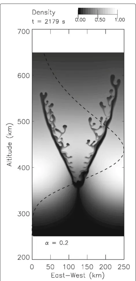
Higher spatial resolution and improved numerical schemes have enabled the simulation of the internal struc-tures of EPBs, which could not be reproduced using pre-vious models. Huba and Joyce (2007) have developed a new code that uses an eighth-order spatial interpolation scheme and the partial donor cell method (Hain 1987). Figure 4 shows a number of secondary bifurcations from the walls of primary depletions. Although turbulent struc-tures were reproduced in this model, V-shaped primary depletions are somewhat unnatural and may have arisen because of the 2D treatment. Around this time, a rapid transition from 2D to 3D modeling studies was underway.
Three-dimensional models
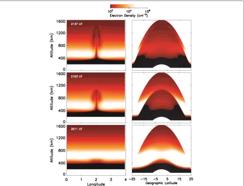
The 2D models presented in the previous section assume that all parameters are uniformly distributed along lati-tude and the magnetic field lines extend to infinity in the horizontal direction. These assumptions are far from the real configuration, in which equatorial ionization anoma-lies and magnetic field curvature are present. The rapid advancement of high-performance computing technology has made it possible to conduct ionospheric simulations in a fully 3D domain. In preliminary 3D simulations of EPBs presented by Keskinen et al. (2003) and Kherani et al. (2005), it was concluded that finite parallel conduc-tivity effects slow the evolution of EPBs. 3D modeling studies of EPBs have been widely recognized since a new model was developed by Huba et al. (2008) based on the global ionosphere model SAMI3. As shown in Fig. 5,
Fig. 4Small-scale structures inside EPBs. The model here used an eighth-order spatial interpolation scheme and the partial donor cell method. Reproduced from Huba and Joyce (2007)
Fig. 5The first full 3D simulation of EPBs. The geographic and geomagnetic latitudes coincide with each other. Reproduced from Huba et al. (2008)
the decay phase of EPBs (Krall et al. 2010a, b), and the electrostatic reconnection process of merging EPBs (Huba et al. 2015).
The seeding of EPBs by collisional shear instabilities has been studied by Hysell et al. (2006) using a model that includes finite parallel conductivity effects. The model was extended by Aveiro and Hysell (2010) to repro-duce the nonlinear evolution of EPBs seeded by colli-sional shear instabilities. Because the non-equipotential solution provides the 3D current system in the model, including diamagnetic and field-aligned currents, the magnetic signatures inside EPBs can also be reproduced (Aveiro et al. 2011; Yokoyama and Stolle 2017). Aveiro and Hysell (2012) and Aveiro and Huba (2013) further examined the difference between the equipotential and equipotential solutions and concluded that the non-equipotential solution contributed to the formation of complex EPB structures. The model was also applied to the evaluation of actual observations by adopting
pre-sunset observation data to define the initial conditions (Aveiro et al. 2012; Hysell et al. 2014b, c, 2015). This data assimilation approach may greatly strengthen the probability of forecasting the occurrence of EPBs.
Off-equatorial phenomena, that is, sporadic-E (Es)
lay-ers and medium-scale traveling ionospheric disturbances (MSTIDs), have also been proposed as seeding sources of ESF and EPBs via electric field mapping along geo-magnetic field lines (Tsunoda 2007; Miller et al. 2009). A preliminary modeling study has been conducted by using the SAMI3/ESF model with artificially imposed MSTID structures in off-equatorial regions (Krall et al. 2011). These effects could be quantitatively investigated by coupling the 3D ESF models with high-resolution midlatitude models (e.g., Yokoyama and Hysell 2010) that can numerically reproduce the Es-layer instability
and MSTIDs.
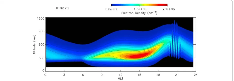
An interesting approach is to resolve EPBs in a global ionospheric model. Huba and Joyce (2010) modified the dusk sector of the global SAMI3 model to have a higher spatial resolution (approximately 7 km). Owing to the self-consistent treatment of global electrodynamics and the formation of EPBs in this method, large-scale EPBs are generated successively at the dusk sector as shown in Fig. 6. This method coupled with a global thermosphere model would be a strong tool to assess the possibility of EPB occurrence.
The most recent 3D model is the High-Resolution Bub-ble (HIRB) model developed by Yokoyama et al. (2014). Adopting a spatial resolution as fine as 1 km and the CIP scheme for plasma transport, the HIRB model is capable of reproducing EPBs that grow nonlinearly from the crest of a large-scale upwelling, bifurcate at the top of EPBs, then become turbulent at the topside of the F region. Figure 7 shows the plasma density distribution of fully developed EPBs in a 3D domain. This distribu-tion shows that depledistribu-tions contain very turbulent struc-tures that are elongated along magnetic flux tubes and reach off-equatorial latitudes. Applying multiple seeding components and an eastward neutral wind, east–west
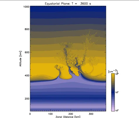
asymmetry, and tilted structures can also be reproduced, as shown in Fig. 8 (Yokoyama et al. 2015). Although the outline of tilted EPBs is similar to the previous 2D model, result shown in Fig. 3, their internal structures are markedly different.
Even though computer hardware has been significantly advanced, it is still difficult to simultaneously reproduce the Fresnel scale of L-band signals (300–400 m) and large-scale EPBs (approximately 100 km) in the same model. Retterer (2005) proposed a scintillation forecasting sys-tem based on numerical modeling and satellite obser-vation as a part of the Communication and Navigation Outage Forecasting System (C/NOFS) program. Retterer and Gentile (2009) conducted an EPB simulation with the physics-based model (PBMOD) described in Retterer (2005). The initial background conditions were derived from the global ambient ionospheric model that was used for scintillation forecasting with vertical plasma drifts (Retterer et al. 2005). The simulated EPB occurrence was well correlated with DMSP satellite observations. Retterer (2010a, b) tried to evaluate amplitude scintillation with a phase screen model by extrapolating the density irregular-ity spectra of EPBs simulated by the PBMOD. However, because the spatial resolution of the PBMOD was limited to 2.5 km at most, spectral breaks at the intermediate scale were not observed (e.g., Singh and Szuszczewicz 1984). To extrapolate irregularity spectra down to the Fresnel scale, it is necessary to reproduce smaller-scale irregulari-ties as accurately as possible. The spatial resolution of the HIRB model was improved for this purpose. In the model with improved resolution, the longitudinal axis is divided by 1120 grid points with a grid spacing of 333.6 m. The number of magnetic field lines on the magnetic meridian is increased more than twofold to 1821, and the altitude range of 300 to 800 km over the magnetic equator is uniformly sampled with a spacing of 700.8 m.
Fig. 73D view of HIRB model results. Reproduced from Yokoyama et al. (2014)
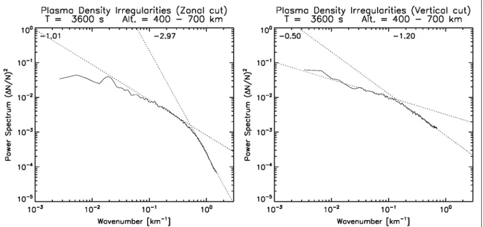
Figure 9 shows a 2D snapshot of the higher reso-lution result under the same conditions as for Fig. 8, demonstrating that more turbulent internal EPB struc-tures can be observed at a higher resolution. The power spectra of the irregularities inside the EPBs were cal-culated along the zonal and vertical coordinates using a simple FFT technique, and they were averaged over altitudes ranging from 400 to 700 km. Figure 10 shows the average power spectra along the zonal and verti-cal coordinates. Spectral breaks appeared near 2 and 8 km for zonal and vertical density irregularities, respec-tively. The break scales are nearly the same as those seen in the previous in situ measurements (Singh and Szuszczewicz 1984). Wavelet-based analysis may provide a better description of the spectral characteristics (Rino et al. 2014, 2016). Analysis of the simulated spectral
characteristics based on wavelet analysis techniques is underway (Rino et al. 2017).
Conclusions
Numerical modeling efforts to understand ESF and EPBs in the past 40 years were reviewed in this article. Since the nonlinear evolution of EPBs was first successfully modeled, various models have been intensively devel-oped and improved because of the rapid advancement of high-performance computing technology and numer-ical algorithms. However, present methods remain far from forecasting the occurrence of EPBs on a day-to-day basis. Some models set up initial background conditions from global ionospheric models, but there are signifi-cant deviations among the existing global models, espe-cially under nighttime conditions (Anderson et al. 1998;
Fig. 10Power spectral density plots of irregularities shown in Fig. 9. The power spectra were calculated using a simple FFT technique for each density profile along the zonal (vertical) coordinates and averaged over altitudes ranging from 400 to 700 km
Fang et al. 2013). This means that the causes of the day-to-day variability of the background ionosphere are not fully reflected in existing global models. It may be necessary to include assimilative techniques from real-time obser-vations to reliably model the background conditions. Fur-thermore, the growth of EPBs in the models strongly depends on how initial seeding perturbations are added. As the required spatial resolution for EPB formation (<10 km) is much finer than that of the global models (>1◦), the use of some artificial inputs as seeding perturbations is unavoidable. It is necessary to employ appropriate back-ground conditions and initial perturbations to conduct reliable forecasting using numerical models, but this is not an easy task.
The recent development of a high-resolution bubble model has made it possible to resolve nearly Fresnel scale irregularities for L-band GNSS signals. Because the spec-tral characteristics of density irregularities inside EPBs do not obey a simple power law, extrapolation from large-scale irregularities cannot be used to accurately esti-mate the scintillation strength. It is necessary to directly resolve Fresnel scale irregularities to quantitatively eval-uate the scintillation. On the other hand, several issues must be addressed for the development of very-high-resolution models. The equipotential assumption may no longer be justified, and the ion inertial term must be included for parallel transport. These terms can be omit-ted for the evolution of large-scale EPBs, but they do affect density irregularities smaller than approximately 100 m.
The next realistic step is to couple global simulation models, in which real-time observation data are assimi-lated, with regional models that can resolve small-scale irregularities. The partially high-resolution global model developed by Huba and Joyce (2010) could be applied relatively easily for forecasting purposes. Regarding the model configuration, the definition of appropriate bound-ary conditions is important because EPBs tend to occur around the dusk terminator, where the eastern and west-ern boundaries should correspond to the nightside and dayside ionospheres, respectively. An understanding of the electrodynamics in the dusk side is still important for EPB forecasting.
If a full high-resolution global simulation model were realized, it could model all phenomena at all scales. Such a model might be realized in the distant future, but we should keep developing state-of-the-art models and pre-pare for the future when super-high-performance com-puters become available.
Abbreviations
AGW: Atmospheric gravity wave; CIP: Constrained interpolation profile; ESF: Equatorial spreadF; EPB: Equatorial plasma bubble; FCT: Flux-corrected transport; GNSS: Global navigation satellite system; HIRB: High-resolution bubble; PBMOD: Physics-based model; SAMI3: Sami3 is also a model of the ionosphere
Acknowledgements
Funding
This work was supported by JSPS KAKENHI Grant Number 16K17814.
Authors’ contributions
TY prepared all parts of the manuscript.
Competing interests
The authors declare that they have no competing interest.
Publisher’s Note
Springer Nature remains neutral with regard to jurisdictional claims in published maps and institutional affiliations.
Received: 30 August 2017 Accepted: 28 November 2017
References
Adams J (1991) Multigrid software for elliptic partial differential equations: MUDPACK. In: NCAR Technical Note-357+STR. National Center for Atmospheric Research, Boulder CO
Anderson DN, Buonsanto MJ, Codrescu M, Decker D, Fesen CG, Fuller-Rowell TJ, Reinisch BW, Richards PG, Roble RG, Schunk RW, Sojka JJ (1998)
Intercomparison of physical models and observations of the ionosphere. J Geophys Res 103:2179–2192
Aveiro HC, Hysell DL (2010) Three-dimensional numerical simulation of equatorialFregion plasma irregularities with bottomside shear flow. J Geophys Res 115:11321. doi:10.1029/2010JA015602
Aveiro HC, Hysell DL, Park J, Lühr H (2011) Equatorial spreadF-related currents: three-dimensional simulations and observations. Geophys Res Lett 38:21103. doi:10.1029/2011GL049586
Aveiro HC, Hysell DL (2012) Implications of the equipotential field line approximation for equatorial spreadFanalysis. Geophys Res Lett 39:11106. doi:10.1029/2012GL051971
Aveiro HC, Hysell DL, Caton RG, Groves KM, Klenzing J, Pfaff RF, Stoneback R, Heelis RA (2012) Three-dimensional numerical simulations of equatorial spreadF: results and observations in the Pacific sector. J Geophys Res 117:03325. doi:10.1029/2011JA017077
Aveiro HC, Huba JD (2013) Equatorial spread F studies using SAMI3 with two-dimensional and three-dimensional electrostatics. Ann Geophys 31:2157–2162. doi:10.5194/angeo-31-2157-2013
Carrano CS, Rino CL (2016) A theory of scintillation for two-component power law irregularity spectra: overview and numerical results. Radio Sci 51:789–813. doi:10.1002/2015RS005903
Duly TM, Huba JD, Makela JJ (2014) Self-consistent generation of MSTIDs within the SAMI3 numerical model. J Geophys Res 119:6745–6757. doi:10.1002/2014JA020146
Dungey JW (1956) Convective diffusion in the equatorialFregion. J Atmos Terr Phys 9:304–310
Fang T-W, Anderson D, Fuller-Rowell T, Akmaev R, Codrescu M, Millward G, Sojka J, Scherliess L, Eccles V, Retterer J, Huba J, Joyce G, Richmond A, Maute A, Crowley G, Ridley A, Vichare G (2013) Comparative studies of theoretical models in the equatorial ionosphere. In: Huba J, Schunk R, Khazanov G (eds). Modeling the Ionosphere-Thermosphere System, Geophysical Monograph Series. American Geophysical Union, Washington. pp 133–144. doi:10.1002/9781118704417.ch12 Farley DT, Balsley BB, Woodman RF, McClure JP (1970) Equatorial spreadF:
implications of VHF radar observations. J Geophys Res 75:7199–7216 Fujino S, Murakami K (2013) A parallel variant of BiCGStar-Plus method
reduced to single global synchronization. AsiaSim 2013 CCIS Ser 402:325–332. doi:10.1007/978-3-642-45037-2_30
Hain K (1987) The partial donor cell method. J Comput Phys 73:131–147 Harten A (1983) High resolution schemes for hyperbolic conservation laws.
J Comput Phys 49:357–393
Hines CO (1960) Internal atmospheric gravity waves at ionospheric heights. Can J Phys 38:1441–1481
Huang CS, Kelley MC (1996a) Nonlinear evolution of equatorial spreadF: 1. On the role of plasma instabilities and spatial resonance associated with gravity wave seeding. J Geophys Res 101:283–292
Huang, CS, Kelley MC (1996b) Nonlinear evolution of equatorial spreadF: 2. Gravity wave seeding of rayleigh–taylor instability. J Geophys Res 101:293–302
Huang CS, Kelley MC (1996c) Nonlinear evolution of equatorial spreadF: 3. Plasma bubbles generated by structured electric fields. J Geophys Res 101:303–313
Huang, CS, Kelley MC (1996d) Nonlinear evolution of equatorial spreadF: 4. Gravity waves, velocity shear, and day-to-day variability. J Geophys Res 101:24521–24532
Huba JD, Joyce G (2007) Equatorial spreadFmodeling: multiple bifurcated structures, secondary instabilities, large density ’bite-outs,’ and supersonic flows. Geophys Res Lett 34:07105. doi:10.1029/2006GL028519
Huba JD, Joyce G, Krall J (2008) Three-dimensional equatorial spreadF modeling. Geophys Res Lett 35:10102. doi:10.1029/2008GL033509 Huba JD, Ossakow SL, Joyce G, Krall J, England SL (2009) Three-dimensional
equatorial spreadFmodeling: zonal neutral wind effects. Geophys Res Lett 36:19106. doi:10.1029/2009GL040284
Huba JD, Joyce G (2010) Global modeling of equatorial plasma bubbles. Geophys Res Lett 37:17104. doi:10.1029/2010GL044281
Huba JD, Krall J (2013) Impact of meridional winds on equatorial spreadF: revisited. Geophys Res Lett 40:1268–1272. doi:10.1002/grl.50292 Huba JD, Wu TW, Makela JJ (2015) Electrostatic reconnection in the
ionosphere. Geophys Res Lett 42:1626–1631. doi:10.1002/2015GL063187 Hysell DL, Jafari R, Fritts DC, Laughman B (2014a) Gravity wave effects on
postsunset equatorialFregion stability. J Geophys Res Space Physics 119:5847–5860. doi:10.1002/2014JA019990
Hysell DL, Jafari R, Milla MA, Meriwether JW (2014b) Data-driven numerical simulations of equatorial spreadFin the Peruvian sector. J Geophys Res Space Phys 119:3815–3827. doi:10.1002/2014JA019889
Hysell DL, Milla MA, Condori L, Meriwether JW (2014c) Data-driven numerical simulations of equatorial spreadFin the Peruvian sector: 2. Autumnal equinox. J Geophys Res Space Phys 119:6981–6993.
doi:10.1002/2014JA020345
Hysell DL (2000) An overview and synthesis of plasma irregularities in equatorial spreadF. J Atmos Sol Terr Phys 62:1037–1056
Hysell DL, Burcham JD (2002) Long term studies of equatorial spreadFusing the JULIA radar at Jicamarca. J Atmos Sol Terr Phys 64:1531–1543 Hysell DL, Kudeki E (2004) Collisional shear instability in the equatorialFregion
ionosphere. J Geophys Res 109:11301. doi:10.1029/2004JA010636 Hysell DL, Larsen MF, Swenson CM, Wheeler TF (2006) Shear flow effects at the
onset of equatorial spreadF. J Geophys Res 111:11317. doi:10.1029/2006JA011963
Hysell DL, Milla MA, Condori L, Vierinen J (2015) Data-driven numerical simulations of equatorial spreadFin the Peruvian sector: 3. Solstice. J Geophys Res Space Phys 120:10809–10822. doi:10.1002/2015JA021877 Kelley MC, Larsen MF, LaHoz C, McClure JP (1981) Gravity wave initiation of
equatorial spread F: a case study. J Geophys Res 86:9087–9100 Kelley MC, Seyler CE, Zargham S (1987) Collisional interchange instability: 2. A
comparison of the numerical simulations with the in situ experimental data. J Geophys Res 92:10089–10094
Kelley MC, Hysell DL (1991) Equatorial spread-Fand neutral atmospheric turbulence: a review and a comparative anatomy. J Atmos Terr Phys 53:695–708
Kelley MC (2009) The Earth’s ionosphere: plasma physics and electrodynamics. 2nd edn. Int Geophys Ser vol 96. Academic Press, Boston
Keskinen MJ, Szuszczewicz EP, Ossakow SL, Holmes JC (1981) Nonlinear theory and experimental observations of the local collisional Rayleigh–Taylor instability in a descending equatorial spreadFionosphere. J Geophys Res 86:5785–5792
Keskinen MJ, Ossakow SL, Fejer BG (2003) Three-dimensional nonlinear evolution of equatorial ionospheric spread-F bubbles. Geophys Res Lett 30(16):1855. doi:10.1029/2003GL017418
Keskinen MJ, Vadas SL (2009) Three-dimensional nonlinear evolution of equatorial ionospheric bubbles with gravity wave seeding and tidal wind effects. Geophys Res Lett 36:12102. doi:10.1029/2009GL037892
Keskinen MJ (2010) Equatorial ionospheric bubble precursor. Geophys Res Lett 37:09106. doi:10.1029/2010GL042963
Kherani EA, Mascarenhas M, Sobral JHA, de Paula ER, Bertoni F (2005) A three-dimensional simulation of collisional-interchange-instability in the equatorial-low-latitude ionosphere. Space Sci Rev 121:253–269. doi:10.1007/s11214-006-6158-x
Kintner PM, Ledvina BM, de Paula ER (2007) GPS and ionospheric scintillations. Space Weather 5:09003. doi:10.1029/2006SW000260
Krall, J, Huba JD, Ossakow SL, Joyce G (2010b) Equatorial spreadFfossil plumes. Ann Geophys 28:2059–2069. doi:10.5194/angeo-28-2059-2010 Krall J, Huba JD, Fritts DC (2013a) On the seeding of equatorial spreadFby
gravity waves. Geophys Res Lett 40:661–664. doi:10.1002/GRL.50144 Krall J, Huba JD, Joyce G, Hei M (2013b) Simulation of the seeding of equatorial
spreadFby circular gravity waves. Geophys Res Lett 40:1–5. doi:10.1029/2012GL054022
Krall J, Huba JD, Joyce G, Zalesak ST (2009) Three-dimensional simulation of equatorial spread-F with meridional wind effects. Ann Geophys 27:1821–1830
Krall J, Huba JD, Ossakow SL, Joyce G, Makela JJ, Miller ES, Kelley MC (2011) Modeling of equatorial plasma bubbles triggered by non-equatorial traveling ionospheric disturbances. Geophys Res Lett 38:08103. doi:10.1029/2011GL046890
Madala RV (1978) An efficient direct solver for separable and non-separable elliptic equations. Mon Wea Rev 106:1735–1741
McDonald BE, Ossakow SL, Zalesak ST, Zabusky NJ (1981) Scale sizes and lifetimes ofFregion plasma cloud striations as determined by the condition of marginal stability. J Geophys Res 86:5775–5784
Miller ES, Makela JJ, Kelley MC (2009) Seeding of equatorial plasma depletions by polarization electric fields from middle latitudes: experimental evidence. Geophys Res Lett 36:18105. doi:10.1029/2009GL039695 Retterer JM (2010a) Forecasting low-latitude radio scintillation with 3-D
ionospheric plume models: 1. Plume model. J Geophys Res 115:03306. doi:10.1029/2008JA013839
Retterer, JM (2010b) Forecasting low-latitude radio scintillation with 3-D ionospheric plume models: 2. Scintillation calculation. J Geophys Res 115:03307. doi:10.1029/2008JA013840
Retterer JM (2005) Physics-based forecasts of equatorial radio scintillation for the communication and navigation outage forecasting system (c/nofs). Space Weather 3:12–03. doi:10.1029/2005SW000146
Retterer JM, Decker DT, Borer WS, Daniell Jr RE, Fejer BG (2005) Assimilative modeling of the equatorial ionosphere for scintillation forecasting: modeling with vertical drifts. J Geophys Res 110:11307.
doi:10.1029/2002JA009613
Retterer JM, Gentile LC (2009) Modeling the climatology of equatorial plasma bubbles observed by DMSP. Radio Sci 44:0–31. doi:10.1029/2008RS004057 Retterer JM, Roddy P (2014) Faith in a seed: on the origins of equatorial plasma
bubbles. Ann Geophys 32:485–498. doi:10.5194/angeo-32-485-2014 Rino CL, Tsunoda RT, Petriceks J, Livingston RC, Kelley MC, Baker KD (1981)
Simultaneous rocket-borne beacon and in situ measurements of equatorial spreadF—intermediate wavelength results. J Geophys Res 86:2411–2420 Rino CL, Carrano CS, Roddy P (2014) Wavelet-based analysis and power law
classification of C/NOFS high-resolution electron density data. Radio Sci 49:680–688. doi:10.1002/2013RS005272
Rino CL, Carrano CS, Groves KM, Roddy PA (2016) A characterization of intermediate-scale spreadFstructure from four years of high-resolution C/NOFS satellite data. Radio Sci 51:779–788. doi:10.1002/2015RS005841 Rino CL, Yokoyama T, Carrano CS (2017) Characteristics of high-resolution
simulated equatorial plasma bubbles. Prog Earth Planet Sci. (in press) Saad Y (1990) SPARSKIT: a basic tool kit for sparse matrix computations. In:
Tech. Rep. RIACS-90-20. Research Institute for Advanced Computer Science, NASA Ames Research Center, Moffett Field
Saad Y (2003) Iterative Methods for Sparse Linear Systems. 2nd edn. SIAM Publications, Philadelphia
Scannapieco AJ, Ossakow SL (1976) Nonlinear equatorial spread F. Geophys Res Lett 3:451–454
Sekar R, Suhasini R, Raghavarao R (1994) Effects of vertical winds and electric fields in the nonlinear evolution of equatorial spreadF. J Geophys Res 99:2205–2213
Sekar R (2003) Plasma instabilities and their simulations in the equatorialF region—recent results. Space Sci Rev 107:251–262
Singh M, Szuszczewicz EP (1984) Composite equatorial spreadFwave number spectra from medium to short wavelength. J Geophys Res 89:2313–2323 Stolle C, Lühr H, Rother M, Balasis G (2006) Magnetic signatures of equatorial spreadFas observed by the CHAMP satellite. J Geophys Res 111:02304. doi:10.1029/2005JA011184
Sultan PJ (1996) Linear theory and modeling of the Rayleigh–Taylor instability leading to the occurrence of equatorial spreadF. J Geophys Res 101:26875–26891
Tsunoda RT, White BR (1981) On the generation and growth of equatorial backscatter plumes 1. Wave structure in the bottomsideFlayer. J Geophys Res 86:3610–3616
Tsunoda, RT (2007) Seeding of equatorial plasma bubbles with electric fields from anes-layer instability. J Geophys Res 112:06304.
doi:10.1029/2006JA012103
Tsunoda RT (2015) Upwelling: a unit of disturbance in equatorial spreadF. Prog Earth Planet Sci 2:9. doi:10.1186/s40645-015-0038-5
Woodman RF, LaHoz C (1976) Radar observations ofFregion equatorial irregularities. J Geophys Res 81:5447–5466
Woodman RF (2009) Spread F—an old equatorial aeronomy problem finally resolved? Ann Geophys 27:1915–1934
Yabe T, Xiao F, Utsumi T (2001) The constrained interpolation profile method for multiphase analysis. J Comput Phys 169:556–593
Yabe T, Mizoe H, Takizawa K, Moriki H, Im H-N, Ogata Y (2004) Higher-order schemes with CIP method and adaptive Soroban grid towards mesh-free scheme. J Comput Phys 194:57–77
Yeh KC, Liu C-H (1982) Radio wave scintillations in the ionosphere. Proc IEEE 70:324–360
Yokoyama T, Hysell DL (2010) A new midlatitude ionosphere electrodynamics coupling model (MIECO): latitudinal dependence and propagation of medium-scale traveling ionospheric disturbances. Geophys Res Lett 37:08105. doi:10.1029/2010GL042598
Yokoyama T, Shinagawa H, Jin H (2014) Nonlinear growth, bifurcation, and pinching of equatorial plasma bubble simulated by three-dimensional high-resolution bubble model. J Geophys Res Space Phys
119:10474–10482. doi:10.1002/2014JA020708
Yokoyama T, Jin H, Shinagawa H (2015) West wall structuring of equatorial plasma bubbles simulated by three-dimensional HIRB model. J Geophys Res Space Physics 120:8810–8816. doi:10.1002/2015JA021799
Yokoyama T, Stolle C (2017) Low and midlatitude ionospheric plasma density irregularities and their effects on geomagnetic field. Space Sci Rev 206:495–519. doi:10.1007/s11214-016-0295-7
Zalesak ST (1979) Fully multidimensional flux-corrected transport algorithms for fluids. J Comput Phys 31:335–362
Zalesak ST, Ossakow SL (1980) Nonlinear equatorial spreadF: spatially large bubbles resulting from large horizontal scale initial perturbations. J Geophys Res 85:2131–2142
Zalesak ST, Ossakow SL, Chaturvedi PK (1982) Nonlinear equatorial spreadF: the effect of neutral winds and background conductivity. J Geophys Res 87:151–166
Zargham, S, Seyler CE (1987) Collisional interchange instability: 1. Numerical simulations of intermediate-scale irregularities. J Geophys Res 92:10073–10088