Semiparametric Mean Field Variational Bayes: General Principles and Numerical Issues

Semiparametric Mean Field Variational Bayes:

General Principles and Numerical Issues

David Rohde davidjrohde@gmail.com

School of Mathematical and Physical Sciences University of Techonology Sydney

P.O. Box 123, Broadway, 2007, Australia

Matt P. Wand matt.wand@uts.edu.au

School of Mathematical and Physical Sciences University of Techonology Sydney

P.O. Box 123, Broadway, 2007, Australia

Editor:Xiaotong Shen

Abstract

We introduce the termsemiparametric mean field variational Bayes to describe the relax-ation of mean field varirelax-ational Bayes in which some density functions in the product density restriction are pre-specified to be members of convenient parametric families. This notion has appeared in various guises in the mean field variational Bayes literature during its his-tory and we endeavor to unify this important topic. We lay down a general framework and explain how previous relevant methodologies fall within this framework. A major contri-bution is elucidation of numerical issues that impact semiparametric mean field variational Bayes in practice.

Keywords: Bayesian Computing, Factor Graph, form Variational Bayes, Fixed-point Iteration, Non-conjugate Variational Message Passing, Nonlinear Conjugate Gradient Method

1. Introduction

We expound semiparametric mean field variational Bayes, a powerful combination of the notions of minimum Kullback-Leibler divergence and mean field restriction, that allows fast and often accurate approximate Bayesian inference for a wide range of scenarios. Most of its foundational literature and applications are in Machine Learning. However, semiparametric mean field variational Bayes is also an important paradigm for Statistics in the age of very big sample sizes and models.

algorithm for Bayesian Poisson mixed models by pre-specifying the fixed and random effects parameters to have Multivariate Normal distributions. Knowles and Minka (2011) took a message passing approach to mean field variational Bayes and explain how their approach to inclusion of pre-specified parametric families allows modular inference algorithms for ar-bitrary factors. Some recent articles on this topic have used the termsfixed-form variational Bayes (Honkela et al., 2010) and non-conjugate variational message passing (Knowles & Minka, 2011), to describe this modification of mean field variational Bayes. However, in this article we argue for adoption of the termsemiparametric mean field variational Bayes. Although we give a precise mathematical description of semiparametric mean field vari-ational Bayes in Section 2, it simply refers to the relaxation of ordinary mean field varia-tional Bayes in which some of the density functions in the postulated product density form are pre-specified to be particular parametric density functions, often chosen for reasons of tractability. This is a ‘halfway house’ between fully parametric approximation of the joint posterior density function of the model parameters with minimum Kullback-Leibler diver-gence used for parameter choice and pure mean field variational Bayes in which there is no parametric specification at all – only the product restriction. The following comments apply to our general framework:

• Semiparametric mean field variational Bayes is a modification of mean field variational Bayes that could be carried out via a message passing approach, as done by Knowles and Minka (2011), or by using the more common q-density approach used in, for example, Bishop (2006) and Ormerod and Wand (2010).

• The notion of conjugacy is not intrinsic to semiparametric mean field variational Bayes. The principle may be applied regardless of conjugacy relationships amongst the messages and/orq-densities. Therefore, the ‘non-conjugacy’ label used in recent articles for semiparametric relaxations of mean field variational Bayes is somewhat misleading.

• Contributions such as Knowles and Minka (2011) and Tan and Nott (2013) restrict attention to pre-specification of parametric families that are of exponential family form (e.g. Wainwright and Jordan, 2008). Whilst exponential family density functions have tractability advantages when used in semiparametric mean field variational Bayes, there is no intrinsic reason for only such densities to be used. In Section 5 we illustrate this point using pre-specified Skew-Normal density functions, which are not within the exponential family.

• Recent articles on non-conjugate variational message passing, such as Knowles and Minka (2011), Tan and Nott (2013) and Menictas and Wand (2015) used fixed-point iteration to minimize the Kullback-Leibler divergence or, equivalently, maximize the lower bound on the marginal log-likelihood. Theorem 1 of Knowles and Minka (2011) constitutes such an approach. However, any optimization approach could be used for obtaining the Kullback-Leibler optimal parameters such as Newton-Raphson iteration, quasi-Newton iteration, stochastic gradient descent, the Nelder-Mead simplex method and various hybrids and modifications of such methods.

the posterior is within a parametric family such as Multivariate Normal with banded Cholesky covariance matrix factors. These contributions represent special cases of semiparametric mean field variational Bayes and their findings have relevance to the more general situation.

The main purposes of this article are:

(1) Bring together the literature on semiparametric mean field variational Bayes and identify its core tenets.

(2) Lay out and discuss numerical issues that arise in semiparametric mean field varia-tional Bayes, which have a significant practical implications for this body of method-ology.

The resulting exposition constitutes the first compendium on semiparametric mean field variational Bayes at its fullest level of generality. It can also be used as a basis for enhance-ments of semiparametric mean field variational Bayes methodology.

We use two examples to elucidate the general principles and numerical issues. The first, Example 1, involves a Bayesian model with a single parameter and, hence, is such that mean field approximation is not required. The simplicity of Example 1 allows a deep appreciation of the various issues with minimal notational overhead. Example 2 is the Bayesian Poisson mixed model treated in Wand (2014) and benefits from semiparametric mean field variational Bayes methodology. It demonstrates issues with high-dimensional optimization problems that are intrinsic to practical implementation.

One of the main outcomes of our numerical investigations is that fitting exponential family density functions via natural fixed-point iteration has some attractive properties. By ‘natural’, we mean a simple version of fixed-point iteration that arises when natural parametrizations are used. As we explain in Section 4, natural fixed-point iterations use Riemanniangradients to step through the parameter space, which is generally more efficient than ordinary gradients. The benefits of Riemannian gradient-based algorithms for Machine Learning problems goes back at least to Amari (1998). Such algorithms are the basis of the semiparametric mean field variational Bayes approach of Honkela et al. (2010).

In Section 2 we describe semiparametric mean field variational Bayes in full generality. A general overview of optimization strategies, pertinent to semiparametric mean field vari-ational Bayes, is given in Section 3. The important special case of pre-specified exponential family density functions is treated in Section 4. Section 5 deals with the more difficult non-exponential family case via an illustrative example. Some closing remarks are given in Section 6.

2. General Principles

Semiparametric mean field variational Bayes is an approximate Bayesian inference method based on the principle of minimum Kullback-Leibler divergence. For arbitrary density functions p1 and p2 on Rd,

KL(p1kp2)≡

Z

Rd

p1(x) log

denotes theKullback-Leibler divergence ofp2 from p1. Note that

KL(p1kp2)≥0 for any p1 and p2. (1) Consider a generic Bayesian model with observed dataDDD and parameter vector (θ,φ). The reason for this notational decomposition of the parameter vector will soon become apparent. Throughout this section we assume that (θ,φ) and DDD are continuous random vectors with density functionsp(θ,φ) and p(DDD). The situation where some components are discrete has similar treatment with summations replacing integrals. Bayesian inference for θ and φis based on the posterior density function

p(θ,φ|DDD) = p(DDD,θ,φ) p(DDD) .

The denominator, p(DDD), is usually referred to as themarginal likelihood or the model evi-dence.

Let q(θ,φ) be an arbitrary density function over the parameter space of (θ,φ). The essence of variational approximate inference is to restrict q(θ,φ) to some class of density functions Qand then use the optimal q-density function, given by

q∗(θ,φ) = argmin q∈Q

KL

n

q(θ,φ)

p(θ,φ|DDD) o

, (2)

as an approximation to the posterior density function p(θ,φ|DDD).

Simple algebraic arguments (e.g. Section 2.1 of Ormerod and Wand, 2010) lead to logp(DDD) = KLnq(θ,φ)

p(θ,φ|DDD) o

+ logp(DDD;q) (3) where

p(DDD;q)≡exp

Z Z

q(θ,φ) log

p(y,θ,φ) q(θ,φ)

dθdφ

. (4)

From (1) we have

p(DDD;q)≤p(DDD) for any q(θ,φ)

showing that p(DDD;q) is a lower bound on the marginal likelihood. The non-negativity condition (1) means that an equivalent form for the optimalq-density function is

q∗(θ,φ) = argmax q∈Q

p(DDD;q). (5)

This alternative optimization problem has the attractive interpretation of q∗(θ,φ) being chosen to maximize a lower bound on the marginal likelihood. For the remainder of this article we work with (5) rather than (2).

Parametric variational approximate inference involves setting

Q={q(θ,φ;ξ) :ξ∈Ξ},

corresponding to a parametric family of density functions with parameter vectorξ ranging over Ξ. In this case (5) reduces to

q∗(θ,φ) = argmax ξ∈Ξ

wherep(DDD;q,ξ) is the marginal likelihood lower bound defined by (4), but with the depen-dence onξ reflected in the notation.

An early contribution of this type is Hinton and van Camp (1993) who used minimum Kullback-Leibler divergence for Gaussian approximation of posterior density functions in neural networks models. Gaussian Q families have also been used by Lappalainen and Honkela (2000), Archambeau et al. (2007), Raiko et al. (2007), Nickisch and Rasmussen (2008), Honkela and Valpola (2005), Honkela et al. (2007), Honkela et al. (2008) and Opper and Archambeau (2009). The recent contribution by Challis and Barber (2013) is an in-depth coverage of Gaussian minimum Kullback-Leibler approximate inference. Salimans and Knowles (2013) devised a stochastic approximation algorithm for solving (6) whenQis a parametric family of exponential family form. Gershman et al. (2012) and Zobay (2014) investigated Gaussian-mixture extensions.

In what one may label a nonparametric variational approximation approach, ordinary mean field variational Bayes uses restricted q-density spaces such as

Q={q(θ,φ) :q(θ,φ) =q(θ1)· · ·q(θM)q(φ)} for some partition{θ1, . . . ,θM} of θ. (7) The word ‘nonparametric’ is justified by the fact that there is no pre-specification that the q-density, or any of its factors, belong to a particular parametric family. Restriction of q(θ,φ) to a product density form is the only pre-specification being made. An iterative scheme for solving (5) under (7) follows from the last displayed equation given in Section 10.1.1 of Bishop (2006). The scheme is listed explictly as Algorithm 1 of Ormerod and Wand (2010). Note that a simple adjustment that caters for (θ,φ), rather thanθ, is required for notation being used here. Gershman et al. (2012) also use the word ‘nonparametric’ to describe a variational approximation approach. However, their methodology is parametric in the sense of the terminology that we are using here.

We propose that the term semiparametric mean field variational Bayes be used for restrictions of the form:

Q={q(θ,φ) :q(θ,φ) =q(θ1)· · ·q(θM)q(φ;ξ), ξ∈Ξ} (8) where {q(φ;ξ) :ξ∈Ξ} is a pre-specified parametric family of density functions in φ. Un-der (8) there is no insistence on theq(θi) having a particular parametric form. For models possessing particular conjugacy properties the optimal q-densities, q∗(θi), will belong to relevant conjugate families. However, in general, the optimal q-densities of the θi can as-sume arbitrary forms; see, for example, Figure 6 of Pham et al. (2013). The quality of a variational approximation is limited by the restrictions imposed by the particular choice of

Q. Semiparametric mean field variational Bayes imposes a product density restriction and then a parametric constraint on one of the factors. The overall quality of the approximation is determined by the combination of these two restrictions. While the estimated nonpara-metric factors are optimal given the product restriction, a paranonpara-metric restriction with fewer product assumptions may be more accurate.

We now turn to the practical problem of solving the optimization problem (5) when the q-density restriction is of the form (8). Appropriate strategies for solving (5) depend on the nature of q(φ;ξ) as a function ofξ and the set Ξ. Some possibilities are:

(B) Ξ is an open subset of Rd for some d ∈ N and q(φ;ξ) is smooth function of ξ over ξ∈Ξ.

(C) Ξ is an open subset of Rd for some d∈N and q(φ;ξ) is a non-smooth function of ξ overξ∈Ξ.

(D) Ξ is a complicated set that does not satisfy any of the descriptions given in (A)–(C). For the vast majority of models in common use andq(φ;ξ) families (B) applies and most of the remainder of this article is devoted to that case. However, we will first briefly deal with (A) in Section 2.1, since it aids understanding of the semiparametric extension of mean field variational Bayes. To date, we are unaware of any semiparametric mean field variational Bayes contributions where (C) or (D) apply, so these cases are left aside.

2.1 Finite Parameter Space Case

Suppose that Ξ is a finite set. Then Algorithm 1 is the natural extension of the mean field variational Bayes coordinate ascent algorithm given, for example, in Section 10.1.1 of Bishop (2006) and Algorithm 1 of Ormerod and Wand (2010). In Algorithm 1, and elsewhere, the notationθ\θi denotes the vectorθ with the entries of θi excluded.

For eachξ∈Ξ:

Initialize: q(θ2), . . . , q(θM). Cycle:

q(θ1)←

exp

E_{q(θ\θ1)q(φ;ξ)}{logp(y,θ,φ)} R

exp

E_q(θ\θ

1)q(φ;ξ){log p(y,θ,φ)}

dθ1 ..

.

q(θM)←

expE_{q(θ\θM)q(φ;ξ)}{log p(y,θ,φ)} R

exp

E_{q(θ\θM)q(φ;ξ)}{log p(y,θ,φ)}

dθM until the increase in p(DDD;q,ξ) is negligible.

q∗(θi;ξ)←q(θi), 1≤i≤M ; p(DDD;q∗,ξ)←p(DDD;q,ξ). ξ∗←argmax

ξ∈Ξ

p(DDD;q∗,ξ) ; q∗(θi)←q∗(θi;ξ∗), 1≤i≤M.

Algorithm 1: Coordinate ascent algorithm for semiparametric mean field variational Bayes when Ξ is a finite parameter space.

2.2 Infinite Parameter Space Case

Algorithm 1 shows how to obtain the Kullback-Leibler-optimal q(θi) and q(φ;ξ) densities in the case where Ξ is finite. However, for common parametric families such as the Normal and Gamma, Ξ is infinite and the solution of (5) under (8) is more delicate. The coordinate ascent idea used to obtain the q∗(θi) in Algorithm 1 can still be entertained. However, it needs to be combined with an optimization scheme that searches for the optimalξ over the infinite space Ξ.

For the remainder of this article we focus on the problem of solving (5) under restric-tion (B) on the q-density parameter space Ξ. We start by studying the criterion function p(DDD;q,ξ) and special forms that it takes under the mean field restriction. The notions of entropy and factor graphs are shown to be very relevant and useful. We then introduce two running examples, Example 1 and Example 2, to illustrate the issues involved. Since Example 1 has only one parameter requiring inference, this is not a fully-fledged semipara-metric mean field variational Bayes problem and the optimization problem is of the form (6). Additionally, (6) for Example 1 is a bivariate optimization problem which allows deeper probing of the numerical analytic issues. Example 2 uses the Poisson mixed model, treated in Section 5.1 of Wand (2014), as our main semiparametric mean field variational Bayes example. It is substantial enough to convey various practical issues but also has a closed form logp(q;ξ) expression that allows purely algebraic exposition.

2.2.1 Entropy, Factor Graphs and the Marginal Log-Likelihood Lower Bound

If xis a random vector having density function p then the corresponding entropy is given by

Entropy(p)≡Ep{−log p(x)}.

For many common distributional families, the entropy admits an algebraic expression in terms of the distribution’s parameters. For example, if

p(x;µ,Σ) = (2π)−d/2|Σ|−1/2 exp{−1₂(x−µ)T Σ−1(x−µ)}

is the Multivariate Normal density function of dimensiondwith mean vectorµand covari-ance matrixΣ then

Entropy(p;µ,Σ) = 1₂d{1 + log(2π)}+1₂log|Σ|. (9) Note that the entropy is independent of the mean vector µ.

Another entropy expression, which arises in many Bayesian models and the example of Section 2.2.3, is that for the Inverse Gamma family of density functions. Let

x∼Inverse-Gamma(κ, λ) denote the random variablex having density function

p(x;κ, λ) = κ λ

Γ(κ)x

with parametersκ, λ >0. In this case

Entropy(p;κ, λ) = log(λ) +κ+ log{Γ(κ)} −(κ+ 1)digamma(κ) (10) where digamma(x)≡(d/dx) log Γ(x) is the digamma function.

The next relevant concept is that of a factor graph, which we first explain via an exam-ple. Consider the approximate Bayesian inference problem according to the semiparametric mean field variational Bayes restriction (8). Figure 1 is the factor graph for an M = 9 example of (8) with the joint density function of all random vectors in the model factorizing as follows:

p(x,θ,φ) = f1(θ1)f2(θ1,θ2,φ)f3(θ3)f4(θ4)f5(θ5,φ)f6(θ5)f7(θ6,φ)f8(θ6)

×f9(θ7,θ8,θ9)f10(θ2,θ3,θ4) (11) forfactors f1, . . . , f10. Note that some of these factors depend on the data vectorx, but the dependence is suppressed in the fj notation. Specific examples are given in Sections 2.2.2 and 2.2.3. In Figure 1 the circles correspond to the components of the mean field product restriction

q(φ) 9

Y

i=1

q(θi) (12)

and are calledstochastic nodes. The solid squares correspond to the factorsfj, 1≤j≤10, and are called factor nodes. Edges join each factor node fj to those stochastic nodes that are included in thefj function.

θ

θ

θ

θ

θ

θ

θ

θ

_θ

9

φ

f

f

f

f

f

f

f

f

f

f

Now consider the general case with semiparametric mean field restriction (8) and suppose thatp(x,θ, φ) hasN factorsfj, 1≤j≤N. Then the marginal log-likelihood lower bound admits the following expression in terms of the components of the corresponding factor graph:

logp(DDD;q,ξ) = Entropy{q(φ;ξ)}+ M

X

i=1

Entropy{q(θi)}+ N

X

j=1

Eq{log(fj)}.

The φ-localized component of logp(DDD;q,ξ), which we denote by logp(DDD;q,ξ)[φ], is logp(DDD;q,ξ)[φ]≡Entropy{q(φ;ξ)}+ X

j∈neighbors(φ)

Eq{log(fj)} (13)

where

neighbors(φ) ≡ {1≤j≤N :fj is a neighbor ofφon the factor graph} = {1≤j≤N :fj involvesφ}.

For the factor graph shown in Figure 1 neighbors(φ) ={2,5,7} and so have

logp(DDD;q,ξ)[φ]= Entropy{q(φ;ξ)}+Eq{log(f2)}+Eq{log(f5)}+Eq{log(f7)}. as theφ-localized component of logp(DDD;q,ξ).

For large Bayesian models it is prudent to maximize this localized approximate log-likelihood as part of a coordinate ascent scheme involving allq-density parameters. Such an approach, combined with the locality property of mean field variational Bayes (e.g. Wand et al., 2011, Section 3), allows for streamlined handling of arbitrarily large models. We formalize this approach to semiparametric mean field variational Bayes in the shape of Algorithm 2 in the upcoming Section 2.2.4. However, we first give some concrete examples of mean field variational Bayes with pre-specified parametric familyq-density functions.

2.2.2 Example 1: Gumbel Random Sample

A Bayesian model for a random samplex1, . . . , xnfrom a Gumbel distribution with location parameterφand unit scale is

p(x1, . . . , xn|φ) = n

Y

i=1

exp{−(xi−φ)−e−(xi−φ)}, φ∼N(µφ, σφ2). (14)

The posterior density function of φis

p(φ|x) =

expnn φ−eφPn

i=1e−xi−2σ12

φ

(φ−µφ)2

o

R∞ −∞exp

n

n φ0−eφ0Pn

i=1e−xi− 1 2σ2

φ

(φ0−µφ)2

o

dφ0

. (15)

and corresponding credible sets. Instead we consider minimum Kullback-Leibler divergence approximation of p(φ|x) over a parametric pre-specified family. Let

Q={q(φ;ξ) :ξ∈Ξ}

be such a parametric family. Then the optimal q-density is q(φ;ξ∗) where ξ∗ = argmax

ξ∈Ξ

p(q;ξ). (16)

Figure 2 shows the factor graph of the model, with factorsp(φ) andp(x|φ) neighboring the stochastic nodeφ.

p(

φ

)

φ

p(

x

|

φ

)

Figure 2: Factor graph for the Example 1 model.

The marginal log-likelihood lower bound is

log p(x;ξ) = Entropy{q(φ;ξ)}+Eq{log p(φ)}+Eq{log p(x|φ)} (17) and the contributions to logp(x;ξ) from the factors are

Eq{logp(φ)} = −_2σ12

φ

h

{Eq(φ;ξ)(φ)−µφ}2+ Varq(φ;ξ)(φ)

i

and Eq{log p(x|φ)} = n Eq(φ;ξ)(φ)−Mq(φ;ξ)(1)Pni=1 e−xi−nx

(18)

whereMq(φ;ξ) is the moment generating function corresponding toq(φ;ξ). Now suppose that

Q=

  

q(φ;µ_q(φ), σ2_q(φ)) = _q 1 2πσ2_q(φ)

exp

(

−(φ−µq(φ))2 2σ2_q(φ)

)

:µ_q(φ) ∈R, σq2(φ)>0

  

corresponding to the Normal family with q-density parameter vectorξ = (µq(φ), σq2(φ)) and parameter space Ξ =R×R+ whereR+ ≡(0,∞) is the positive half-line. Then, from the entropy result (9) and the well-known expression for the moment generating function of the Normal distribution we obtain

logp(x;µq(φ), σ2q(φ)) =12{1 + log(2π)}+ 1 2log(σ

2

q(φ)) +n µq(φ)

−exp(µq(φ)+1₂σ2q(φ)) n

X

i=1

e−xi₋ 1 2σ2

φ

{(µq(φ)−µφ)2+σ_q2_(φ)} −n x.

It follows that the Kullback-Leibler optimal Normalq-density function isq(φ;µ∗_q(φ),(σ2 q(φ))

∗₎

where

"

µ∗_q(φ) (σ2_q(φ))∗

#

= argmax µq(φ)∈R,σ2

q(φ)>0

(

f_Ex1N µq(φ), σ2q(φ);n, n

X

i=1

e−xi_{, µ} φ, σ2φ

!)

and

f_Ex1N (x, y;a, b, c, d) = 1₂log(y) +a x−bexp(x+1₂y)−₂1_d{(x−c)2+y}. (20) The main arguments satisfy x ∈ _R, y > 0 and the auxiliary arguments are such that a, b, d > 0 and c ∈ _R. From (19) we see that the minimum Kullback-Leibler divergence problem (16), whereQ is the Normal family, reduces to a non-linear bivariate optimization problem. Theory given in Challis and Barber (2013) applies to this example. For example, results given in their Section 3.2 can be used to establish that f_Ex1N (x, y;a, b, c, d) is jointly concave in xand √y.

In Section 3 we study strategies for solving such problems and apply them to this example in Section 4.2.

2.2.3 Example 2: Poisson Mixed Model

A single variance componentPoisson mixed model is yi|β,u

ind.

∼ Poisson[exp{(Xβ+Zu)i}], 1≤i≤n, u|σ2∼N(0, σ2IK), σ2|a∼Inverse-Gamma(1₂,1/a),

β∼N(0, σ_β2Ip), a∼Inverse-Gamma(1₂,1/A2)

(21)

whereX is ann×pfixed effects design matrix,Z is ann×K random effects design matrix. Note that the prior onσ in (21) is the Half Cauchy distribution with scale parameter A:

p(σ) = (2/π)

A{1 + (σ/A)2_}, σ >0.

In (21)σβ >0 andA >0 are hyperparameters to be chosen by the analyst.

A mean field approximation to the joint posterior density function of the model param-eters is

p(β,u, σ2, a|y) ≈ q(β,u)q(σ2)q(a). (22) As detailed in Appendix A.3, the optimalq-density functions satisfy

q∗(σ2) andq∗(a) are both Inverse-Gamma density functions, and q∗(β,u)∝exp

yT(Xβ+Zu)−1T exp(Xβ+Zu)

−1₂σ_β−2kβk2₋1

2Eq(σ2)(1/σ

2_)kuk2 _.

(23)

Since q∗(β,u) is not a standard form, numerical methods are required to obtain the varia-tional approximate Bayes estimates and credible sets. Semiparametricmean field variational Bayes alternatives take the form

p(β,u, σ2, a|y) ≈ q(β,u;ξ)q(σ2)q(a) (24) where {q(β,u;ξ) : ξ ∈ Ξ} is a pre-specified parametric family of density functions. The optimal density functionsq(β,u;ξ∗), q∗(σ2) and q∗(a) are found by minimizing

KL

n

q(β,u;ξ)q(σ2)q(a)

p(β,u, σ

We now focus on solving (25).

In Appendix C of Wand (2014) it is shown that

q∗(σ2) is an Inverse-Gamma(1₂(K+ 1), B_q(σ2₎) density function, and

q∗(a) is an Inverse-Gamma(1, Bq(a)) density function where

B_q(σ2₎= 1

2[kEq(β,u;ξ)(u)k

2_{+ tr{Cov}

q(β,u;ξ)(u)}] +µq(1/a) (26) and Bq(a)=µq(1/σ2₎+A−2 with the definition

µq(1/v)≡Eq(v)(1/v) for a generic random variable v.

(

β

,

u

)

_p(β,

_u

_|σ

_σ

_a

)

p(

y

|β,

u

)

p(σ

|a)

p(a)

Figure 3: Factor graph for the Example 2 model with stochastic nodes corresponding the mean field restriction (24). The dashed line box contains the stochastic node (β,u) and its neighboring factors.

It remains to obtain the optimal value ofξinq(β,u;ξ). Figure 3 shows the factor graph of the current model under mean field restriction (24). The lower bound on the marginal log-likelihood, in terms of the stochastic nodes and factors of Figure 3, is

logp(y;q,ξ) = Entropy{q(β,u;ξ)}+ Entropy{q(σ2)}+ Entropy{q(a)}

+Eq{logp(y|β,u)}+Eq{logp(β,u|σ2)} +Eq{logp(σ2|a)}+Eq{logp(a)}.

(27)

One could substitute (26) into the log p(y;q,ξ) expression. This resulting marginal log-likelihood lower bound would depend on the q-densities only throughξ and could then be maximized overξ ∈Ξ.

An alternative strategy, that scales better to larger models, is to use a coordinate ascent scheme that maximizes log p(y;q,ξ)[(β,u)], the (β,u)-localized component of log p(y;q,ξ), overξ∈Ξ. The relevant factors are those neighboring (β,u) in Figure 3, corresponding to the dashed line box. The quantity requiring maximization is then

logp(y;q,ξ)[(β,u)] = Entropy{q(β,u;ξ)}+Eq{logp(y|β,u)}+Eq{logp(β,u|σ2)} = Entropy{q(β,u;ξ)}+yT_{XE

q(β,u;ξ)(β) +ZEq(β,u;ξ)(u)}

−1TEq(β,u;ξ){exp(Xβ+Zu)}

− 1

2σ2

β

kE_q(β,u;ξ)(β)k2_{+ tr{Cov}

q(β,u;ξ)(β)}

−1₂µq(1/σ2₎

kEq(β,u;ξ)(u)k2+ tr{Covq(β,u;ξ)(u)}

+ const

where ‘const’ denotes terms not depending onξ.

Next, suppose thatQcorresponds to the family of Multivariate Normal density functions in (β,u):

q(β,u;µ_q(β,u),Σq(β,u)) = (2π)−(p+K)/2|Σq(β,u)|−1/2

×exp

(

−1₂

β u

−µ_q(β,u)

T

Σ−_q(1_β,u)

β u

−µ_q(β,u)

)

.

Then the (β,u)-localized approximate marginal log-likelihood reduces to logp(y;q,µ_q(β,u),Σq(β,u))[(β,u)] = 1₂log|Σq(β,u)|+yTCµq(β,u)

−1T exp

n

Cµ_q(β)+1₂diagonal(CΣq(β,u)CT)

o

− 1

2σ2

β

n

kµ_q(β)k2_{+ tr(Σ} q(β))

o

−1₂µq(1/σ2₎

n

kµ_q(u)k2_{+ tr(Σ} q(u))

o

+ const

(29)

whereC ≡[X Z], diagonal(M) is the vector containing the diagonal entries of the square matrixM, andµ_q(β)is the sub-vector ofµ_q(β,u) corresponding toβ. Analogous definitions apply toµ_q(u),Σ_q(β) andΣ_q(u). Appendix A.3 provides derivational details for (29).

For this example, the full coordinate ascent scheme has updates as follows: perform one or more updates of (µ_q(β,u),Σ_q(β,u)) within an iterative scheme for the optimization problem:

argmax µ0_q(β,u),Σ0_q(β,u)

n

log p(y;q,µ0_q(β,u),Σ0_q(β,u))[β,u]

o

B_q(a)←µ_q(1/σ2₎+A−2 ; µ_q(1/a) ←1/B_q(a)

Bq(σ2₎← 1₂[kµ_q(u)k2+ tr{Σ_q(u)}] +µ_q(1/a)

µq(1/σ2₎← ₂1(K+ 1)/B_q(σ2₎.

For now, we deliberately leave the form of the (µ_q(β,u),Σ_q(β,u)) maximization strategy un-specified. We also allow for one or more updates of an iterative scheme aimed at maximizing log p(y;q,µ0_q(β,u),Σ0_q(β,u))[β,u], rather than iterating to convergence at every iteration of the full coordinate ascent scheme. Section 3 describes various optimization strategies that could be used for updating (µ_q(β,u),Σq(β,u)).

Negligible absolute change in log p(y;q,µ_q(β,u),Σq(β,u)) can be used as a stopping cri-terion for the iterations and an algebraic expression for this quantity is given in Appendix A.3.

We return to Example 2 in Section 4.3.

2.2.4 General Semiparametric Mean Field Variational Bayes Algorithm

factor graph ofp(x,φ,θ) with stochastic nodesθ1, . . . ,θM andφ. Algorithm 2 is a general coordinate ascent algorithm for approximate inference that builds on the standard mean field variational Bayes algorithm.

Initialize: q(θ2), . . . , q(θM). Cycle:

perform one or more updates ofξwithin an iterative scheme for the optimization problem:

argmax ξ0∈Ξ

n

logp(DDD;q,ξ0)[φ]o

q(θ1)← exp

E_{q(θ\θ1)q(φ;ξ)}{log p(y,θ,φ)} R

exp

E_{q(θ\θ1)q(φ;ξ)}{log p(y,θ,φ)}

dθ1 ..

.

q(θM)←

expE_{q(θ\θM)q(φ;ξ)}{logp(y,θ,φ)} R

expE_{q(θ\θM)q(φ;ξ)}{log p(y,θ,φ)}

dθM until the absolute change in logp(DDD;q,ξ) is negligible.

Algorithm 2: The general semiparametric mean field variational Bayes algorithm for restric-tion (8) withlogp(DDD;q,ξ)[φ]_{defined with respect to factor graph of p(x,θ,φ)with stochastic} nodes θ1, . . . ,θM and φ.

For each of these approaches, there remains the practical problem of devising an opti-mization scheme for logp(DDD;q,ξ)[φ] and ensuring that it leads to the optimal parameters being chosen. Section 3 deals with this problem.

2.3 Relationship to Existing Literature

The general principle of semiparametric mean field variational Bayes that we have laid out in this section is not brand new and, in fact, instances of this principle have made appearances in the literature since the late 1990s — although they are few in number. We now briefly survey articles known to us that have a semiparametric mean field variational Bayes component. As we will see, the terminology varies quite considerably.

Honkela et al. (2010) adopt the phrase fixed-form variational Bayes in what is a quite general approach to semiparametric mean field variational Bayes as summarized in their Al-gorithm 1. Optimization of the pre-specified parametric component parameters is achieved using the nonlinear conjugate gradient method, which we describe in Section 3.2. However, Honkela et al. (2010) work with with Riemannian gradients which, they argue, are more efficient than Euclidean gradients.

In Knowles and Minka (2011) the focus is incorporation of pre-specified exponential family distributions whilst preserving the message passing aspect of a modular approach to mean field variational Bayes, known as variational message passing. They arrive at an extension which they label non-conjugate variational message passing. The exponential family distribution parameters are chosen via fixed-point iteration, which we describe in detail in Section 3.1.

Tan and Nott (2013) take a semiparametric mean field variational Bayes approach to approximate inference in Bayesian generalized linear mixed models for grouped data. They use pre-specified Multivariate Normal density functions for the random effects of each group with mean field product restrictions and achieve good approximation accuracy via so-called partially noncentered parameterizations.

In the case of pre-specified Multivariate Normal density functions, Wand (2014) ob-tains an explicit form for the fixed-point iteration scheme of Knowles and Minka (2011) and illustrated its use for the Poisson mixed model described in Section 2.2.3. In Luts and Wand (2015) and Menictas and Wand (2015), semiparametric mean field variational Bayes with Multivariate Normal pre-specification is applied, respectively, to count response semiparametric regression and heteroscedastic semiparametric regression.

2.4 Advantages and Limitations of Algorithm 2

As just described in Section 2.3, Algorithm 2 is a very useful generalization of the ordinary mean field variational Bayes algorithm and allows for tractable handling of a wider class of models. For example, the heteroscedastic nonparametric regression model of Menictas and Wand (2015) is such that ordinary mean field variational Bayes is numerically challenging if one uses the same product restrictions as used in homoscedastic nonparametric regression. The semiparametric mean field variational Bayes extension, based on Multivariate Normal pre-specification of basis function coefficients, leads to an iterative scheme with closed form updates. Simulation studies show very good accuracy compared with Markov chain Monte Carlo-based inference. However Algorithm 2 is not guaranteed to converge and, when it does converge, may result in mediocre approximate Bayesian inference. We close this section by briefly discussing such limitations of Algorithm 2.

In cases where a generic iterative procedure is used to solve argmax_ξ0_∈Ξ{logp(D;q, ξ0)} there is no guarantee that the lower bound is increased in a particular iteration or of convergence in general. As a consequence, the convergence guarantees enjoyed by ordinary mean field variational Bayes algorithms are not shared by their semiparametric extension. As we demonstrate in Section 4.2, convergence does not occur for particular numerical optimization strategies.

circumstances where its accuracy is quite poor. Some examples, with explanations for the inaccuracy, are given in Wang and Titterington (2005) and Neville et al. (2014). Semipara-metric mean field variational Bayes shares this limitation since paraSemipara-metric pre-specification imposes a degradation in accuracy compared with ordinary mean field variational Bayes.

3. Numerical Optimization Strategies

In ordinary mean field variational Bayes, parameter optimization is achieved using a convex optimization algorithm that converges under reasonable assumptions (e.g. Luenberger and Ye, 2008). In the semiparametric extension there is no such convex optimization theory and general numerical optimization has to be called upon to optimize the parameters in the pre-specified parametric density function.

Numerical optimization is a major area of mathematical study with an enormous lit-erature. Recent summaries are given in, for example, Givens and Hoeting (2005) and Ackleh et al. (2010), with the former being geared towards optimization problems arising in Statistics. The choice of optimization method typically is driven by factors such as the smoothness of the function requiring optimization and availability of expressions for low-order derivatives. Optimization methods with derivative information invariably take the form of iterative schemes. Semiparametric mean field variational Bayes often has the luxuries of smoothness and derivative expressions. It is also beneficial to have relatively sim-ple iterative updates given the overarching goal of fast approximate inference. Therefore, we gear our summary of numerical optimization strategies towards simple derivative-based schemes. This is in keeping with the existing literature on parametric and semiparametric variational inference.

Let f : D ⊆_Rd _→

R be a function and consider the problem of finding its maximum or minimum value over a setD0 ⊆D. If all partial derivatives of f exist then a necessary condition for a maximum or minimum in the interior ofD0 is thestationary point condition

∂ ∂xj

f(x) = 0, 1≤j≤d. (30) This converts the optimization problem to a multivariate root-finding problem. However (30) is not a sufficient condition for global optima since local optima and saddle points of f insideD0 also satisfy (30). Properties of f, such as regions where it is concave or convex, can aid the determination of global optima.

Throughout this section we make use of the derivative matrix and Hessian matrix no-tation defined in Appendix A.2.

3.1 Fixed-Point Iteration

Assuming that the derivative vectorDxf(x) (defined formally in Appendix A.1) exists, the stationary point condition (30) can be written

Dxf(x)T =0 (31)

of f. Firstly, (31) is rewritten in the form

x=g(x) (32)

for some function g : D ⊆ Rd → Rd. Given this g, fixed-point iteration simply involves repeated evaluation ofg, as given in Algorithm 3

Initialize: x←xinitfor some xinit∈D.

Cycle:

x←g(x)

until convergence.

Algorithm 3: The fixed-point iteration algorithm in generic form. Note, however, the following issues regarding fixed point iteration:

• For a given stationary point condition (31) there are numerous functions g for which (32) holds. In other words, there are many possible fixed point algorithms available to solve (31).

• Once g and xinit are chosen then the above algorithm is not necessarily guaranteed

to converge to a stationary point x∗. There is a large literature on convergence of fixed-point iterative algorithms and good references on the topic include Section 8.1 of Ortega (1990) and Section 8.2 of Ackleh et al. (2010). For example Theorem 8.1.7 of Ortega (1990) asserts that convergence of Algorithm 3 is guaranteed when xinit is

sufficiently close tox∗, the components of g are differentiable atx∗ and ρ Dxg(x∗)

<1.

Here ρ(A) denotes thespectral radius of the square matrix A, defined to be ρ(A)≡maximum of the absolute values of the eigenvalues of A.

Theorem 8.4 of Ackleh et al. (2010) provides a similar condition in terms of thespectral norm kDxg(x∗)kspecwhere

kAkspec≡

q

largest eigenvalue of ATA.

• There are also theorems that guarantee convergence of Algorithm 3 for particular choices of xinit. If D0 is a closed convex subset of D such that g : D0 → D0, the entries ofDxg(x) are each bounded and continuous on D0 and

sup x∈D0

kDxg(x)kspec≤α <1

then Algorithm 3 will converge from any initial point xinit ∈ D0 (Theorems 8.2 and

Despite this elegant theory, it is difficult to apply in practice with regards to choosingg and xinit so that Algorithm 3 converges. This is exemplified in Section 4.2 when we return

to the Example 1 optimization problem. We also note that kDxg(x)kspec<1 nearx

∗ _{is a}

sufficient but notnecessarycondition for convergence of fixed point iteration. Nevertheless, the function

ρ Dxg(x)

is a useful convergence diagnostic for fixed-point iteration. For instance, ifρ Dxg(x)

1

during the iterations then this would indicate convergence problems and the possibility of non-existence of a fixed pointx∗.

Various adjustments to fixed-point iteration have been proposed to enhance convergence. For example, in the context of semiparametric mean field variational Bayes, Section 7 of Minka & Knowles (2011) describes a damping adjustment.

3.1.1 Newton-Raphson Iteration

Newton-Raphson iteration is a special case of fixed-point iteration for optimizing f with theg function taking the form

gNR(x) =x− {Hxf(x)}

−1_D

xf(x)T (33)

where Hxf(x) denotes the Hessian matrix of f(x) as formally defined in Appendix A.1. Assuming existence of {Hxf(x)}−1, it is easily shown that x = gNR(x) if and only if

Dxf(x)T = 0. This leads to Algorithm 4, which conveys the generic form of Newton-Raphson iteration.

Initialize: x←xinitfor some xinit∈D.

Cycle:

x←x− {Hxf(x)}−1Dxf(x)T until convergence.

Algorithm 4: The Newton-Raphson algorithm in generic form. Some pertinent features of Algorithm 4 are:

• The function gNR in (33) has the property

ρ DxgNR(x

∗₎

= 0 (34)

for stationary pointsx∗, A proof is given in Appendix A.4. Therefore, via Theorem 8.4 of Ackleh et al. (2010), convergence to x∗ is guaranteed from a sufficiently close xinit.

• If xinit is such that Algorithm 4 is convergent to x∗ then, under certain regularity

• Locatingxinit values sufficiently close to x∗ for convergence to occur can be difficult

in practice and it is common to combine Newton-Raphson iteration with more robust optimization strategies, such as the Nelder-Mead simplex method.

• A disadvantage of Newton-Raphson iteration compared with other fixed-point itera-tive schemes is the requirement for second order partial derivaitera-tives, corresponding to the entries of the Hessian matrixHxf(x). A feeling for the type of additional calculus needed is given in Appendix A.7.

• A variant of Newton-Raphson optimization known as damped Newton-Raphson em-ploys line searches (or backtracking) in order to achieve much improved convergence behavior. See, e.g., Section 9.5.2 of Boyd and Vandenberghe (2004).

3.2 Nonlinear Conjugate Gradient Method

The nonlinear conjugate gradient method is based on the conjugate gradient method, an established iterative approach to solving large systems of linear equations (Hestenes and Stiefel, 1952). The former arises from applying the latter to the linear system that arises from optimization of a multivariate quadratic function. Details of the nonlinear conjugate gradient method are given in Section 10.8 of Press et al. (2007). Algorithm 5 lists the Polak-Ribi´ere version of the nonlinear conjugate gradient method for maximization of f overD. Since minimization of f is equivalent to maximization of −f it is straightforward to adapt Algorithm 5 to the minimization problem. We choose the Polak-Ribi´ere form here, but another one is the Fletcher-Reeves form given byβ←(vTcurrvcurr)/(vTprevvprev).

Initialize: x←xinit for somexinit∈D.

vprev←Dxf(x)T ; α←argmax α>0

f(x+αvprev)

x←x+αvprev ; s←vprev

Cycle:

vcurr←Dxf(x)T ; β ←vTcurr(vcurr−vprev)/(vTprevvprev)

s←βs+vcurr ; α←argmax

α>0

f(x+αs) x←x+αs ; vprev←vcurr

until convergence.

Algorithm 5: The nonlinear conjugate gradient method for maximization of the function f with the Polak-Ribi´ere form of the β parameter.

alter-native forms. Nonlinear conjugate gradient methods have been shown to have good global convergence properties (Dai and Yuan, 1999).

3.3 Other Optimization Strategies

Other popular optimization strategies include ascent (or descent) algorithms (e.g. Boyd and Vandenberghe, 2004, Section 9.3), quasi-Newton methods (e.g. Givens and Hoeting, 2005, Section 2.2.2.3), the Gauss-Newton method (e.g. Givens and Hoeting, 2005, Section 2.2.3),stochastic gradient descent (e.g. Bottou, 2004) and theNelder-Mead simplex method (Nelder and Mead, 1965). The last of these has the attraction of not requiring derivatives of f and is generally more robust than derivative-based methods.

3.4 Application to Semiparametric Mean Field Variational Bayes We now focus on the optimization component of Algorithm 2

argmax ξ0∈Ξ

n

logp(DDD;q,ξ0)[φ]o (35) and discuss ways in which numerical optimization strategies described in Sections 3.1–3.3 are applicable.

The stationary condition for the maximizer in (35) is Dξlogp(DDD;q,ξ)[φ]

T =0

and this may be manipulated in any of a number of ways to produce an equation of the form ξ =g(ξ) for some functiong. Fixed-point iteration Algorithm 3 can then be entertained but, as discussed in Section 3.1, converge is not guaranteed for arbitraryg. We study this issue in the context of Examples 1 and 2 in Sections 4.2 and 4.3.

Newton-Raphson iteration involves iterative updates:

ξ←ξ− {Hξlogp(DDD;q,ξ)[φ]}−1Dξlogp(DDD;q,ξ)[φ] T

and so is a candidate for insertion into Algorithm 2 for updating the pre-specified parametric q-density parameters.

Another alternative is, of course, updating ξ according to one or more iterations of the nonlinear conjugate gradient method given by Algorithm 5, or any other iterative optimiza-tion scheme. However, convergence needs to be monitored. For high-dimensional ξ, speed of convergence may be also be an important factor. Next we discuss an adjustment aimed at improving the convergence speed of gradient-based algorithms.

3.4.1 Riemannian Geometry Adjustment

As explained in, for example, Section 6.2 of Murray and Rice (1993) the density function family {q(φ;ξ) :ξ ∈ Ξ} can be viewed as a submanifold of a Riemannian manifold. Rie-mannian manifolds do not necessarily have a flat Euclidean geometry. For example, the Riemannian manifold corresponding to the Univariate Normal family:

  

1

q

2πσ2 q(φ)

exp

(

−(φ−µq(φ))

2 2σ2

q(φ)

)

:µq(φ) ∈R, σ2q(φ)>0

  

hashyperbolic geometry (Murray and Rice, 1993, Example 6.6.2) which iscurved. Therefore notions such as closeness of two members of (36) and steepness of gradients when searching over the parameter space Ξ =R×R+ are not properly captured by the Euclidean geometry notions of distance and slope. Adjustments for the Riemannian geometry of the family often improve convergence of optimization algorithms for solving problems such as (35). More detailed discussion on this issue is given in Section 2.2 of Honkela et al. (2010) and Section 2.3 of Hoffman et al. (2013).

Consider an optimization method that uses gradients of the form Dξlogp(DDD;q,ξ)[φ]

T

to find the direction of steepest descent of the objective function logp(DDD;q,ξ)[φ]. The Riemannian geometry adjustment is to instead use

[−E{Hξ logq(φ;ξ)}]−1Dξlogp(DDD;q,ξ)[φ] T

(37) where the premultiplying matrix is the inverseFisher informationofq(φ;ξ). In the Machine Learning literature (e.g. Amari, 1998) (37) is often labeled the natural or Riemannian gradient of logp(DDD;q,ξ)[φ] _{with respect to ξ and the corresponding geometry is called} information geometry. Ifq(φ;ξ) corresponds to the Univariate Normal family (36) then the Fisher information matrix is diag(σ_q−₍2_φ),₂1σ−_q(4_φ)). Therefore, from (37), the natural gradient of logp(q;µ_q(φ), σ_q2_(φ))[φ]with respect to (µ_q(φ), σ_q2_(φ)) is given by

      

σ_q2_(φ) ∂p(q;µq(φ), σ 2 q(φ))

[φ] ∂µq(φ) 2σ4

q(φ)

∂p(q;µ_q(φ), σ2 q(φ))[φ] ∂σ_q2_(φ)

      

T

. (38)

Honkela et al. (2010) is a major contribution to semiparametric mean field variational Bayes methodology and their Algorithm 1 uses the nonlinear conjugate gradient method (Algorithm 5) with natural gradients rather than ordinary gradients. Via both simple examples and numerical studies, they make a compelling case for the use of natural gradients for optimization of the parameters of the pre-specified parametric q-density function. 3.5 Summary of Semiparametric Mean Field Variational Bayes Ramifications In this section we have discussed several iterative numerical optimization strategies. Any of these are candidates for the updating ξ in the Algorithm 2 cycle. Special mention has been given to the well-known Newton-Raphson iteration since it can achieve very rapid convergence and the nonlinear conjugate gradient method which has been shown to be effective in semiparametric mean field variational Bayes contexts when the Riemmannian geometry adjustment of Section 3.4.1 is employed (Honkela et al., 2010).

used to assess the quality of the scheme. In Section 4 we will explain how a particular fixed-point iteration scheme, which we callnatural fixed-point iteration, has attractive properties whenq(·;ξ) is an exponential family density function. We will also revisit Examples 1 and 2 in Section 4 and make some comparisons among various numerical optimization strategies. Natural fixed-point iteration is seen to perform particularly well.

4. Exponential Family Special Case

We now focus on the important special case where the parametric density function family

{q(φ;ξ) :ξ ∈Ξ} can be expressed in exponential family form:

q(φ;η) = exp{T(φ)Tη−A(η)}h(φ), η∈H, (39) whereηis a one-to-one transformation ofξ andH is the image of Ξ under this transforma-tion. In (39)A(η) is called the log-partition function and h(φ) is called the base measure. For example, the Univariate Normal density function family used in Example 1:

q(φ;µq(φ), σq2(φ)) = 1

q

2πσ2 q(φ)

exp

(

−(φ−µ_q(φ))2 2σ2

q(φ)

)

, µq(φ)∈R, σq2(φ)>0,

can be expressed as (39) with

T(φ) =

φ φ2

, η≡

η1 η2

=

"

µq(φ)/σq2(φ)

−1/(2σ2_q(φ))

#

, A(η) =−1₄η2₁/η2− 1₂log(−2η2)

andh(φ) = (2π)−1/2_{. The natural parameter space isH={(η}

1, η2) :η1 ∈R, η2 <0}. Even though semiparametric mean field variational Bayes can involve pre-specification of an ar-bitrary parametric family, virtually all methodology and examples in the existing literature involves pre-specification within an exponential family. Exponential family distributions also play an important role in the theory of mean field variational Bayes (e.g. Sato, 2001; Beal and Ghahramani, 2006; Wainwright and Jordan, 2008).

Now consider the general factor graph set-up described in Section 2.2.1 with the approx-imate marginal log-likelihood logp(DDD;q,η)[φ] given by (13) but as a function of the natural parameter vectorη. Define

NonEntropy{q(φ;η)} ≡ X

j∈neighbors(φ)

Eq(φ;η){log(fj)}

so that

logp(DDD;q,η)[φ]= Entropy{q(φ;η)}+ NonEntropy{q(φ;η)}.

An advantage of working with exponential family density functions is that the entropy takes the simple form:

Entropy{q(φ;η)}=A(η)−DηA(η)η+E[exp{h(φ)}]

where the notation of Appendix A.2 is being used. Moreover, as shown in Lemma 1 of Appendix A.5, the derivative vector of Entropy{q(φ;η)} is simply

This implies that the stationary point condition

{Dη logp(q;η)[φ]}T =0 (41)

is equivalent to

η={HηA(η)}−1DηNonEntropy{q(φ;η)}T. (42) Algorithm 1 of Knowles and Minka (2011) is a fixed-point iteration scheme based on (42).

One further interesting and useful connection concerns the mean parameter vector τ ≡E{T(φ)}

which is related to the natural parameter vector via τ =DηA(η)T.

Under suitable technical conditions τ is a one-to-one transformation of η. Also the chain rule for differentiation of a smooth function s, listed as Lemma 2 in Appendix A.5, is

Dηs= (Dτs)(Dητ) = (Dτs)Dη{DηA(η)T}= (Dτs)HηA(η). which leads to

Dτs={HηA(η)}−1Dηs. (43) Putting all of these relationships together we have:

Result 1 Let ξ be an arbitrary differentiable one-to-one transformation of η. Then the stationary point condition (41) is equivalent to each the following conditions:

(a) η={HηA(η)}−1DηNonEntropy{q(φ;η)}T,

(b) η={HηA(η)}−1(Dηξ)T DξNonEntropy{q(φ;ξ)}T, (c) η=DτNonEntropy{q(φ;τ)}T and

(d) η= (Dτξ)T DξNonEntropy{q(φ;ξ)}T.

We make the following remarks concerning Result 1:

• Result 1(a) immediately gives rise to the following fixed-point iteration scheme in the natural parameter spaceη∈H:

η← {HηA(η)}−1DηNonEntropy{q(φ;η)}T. (44) We refer to (44) as the natural fixed-point iteration scheme and denote the corre-sponding fixed-point function by

gnat(η)≡ {HηA(η)}

−1_D

ηNonEntropy{q(φ;η)}T.

According to the theory of fixed-point iteration discussed in Section 3.1, convergence of (44) is implied by

ρ Dηgnat(η)

• Result 1(b)–(d) offer the possibility of more convenient forms for the fixed-point up-dates in terms of derivatives of the common parameters or mean parameters. Par-ticularly noteworthy is the fact that Result 1(c)–(d) do not require computation of

{HηA(η)}−1. We make use of this situation for the Multivariate Normal family in Section 4.1.

• The Fisher information of q(φ:η) is

−E{Hηlogq(φ;η)}=HηA(η)

which implies that the natural fixed-point iteration scheme (44) involves updating η according to natural Riemannian gradients of NonEntropy(q;τ). From Result 1(c), an equivalent updating scheme is

η←DτNonEntropy{q(φ;τ)}T

which simply involves updatingηaccording to the direction of maximum slope on the NonEntropy(q;τ) surface in theτ space.

• The forms for the stationary point in Result 1 can also be used to derive iterative Newton-Raphson schemes for maximizing logp(q;η)[φ]_{. An example, corresponding} to Result 1(a) and optimization within theη space, is

η←η−

HηNonEntropy{q(φ;η)} −HηA(η)−(ηT ⊗I)Dηvec{HηA(η)}

−1

×[DηNonEntropy{q(φ;η)}T −HηA(η)η].

The vec operator flattens a square matrix into a column vector and is defined formally in Appendix A.1.

Any of the other optimization methods mentioned in Section 3 can also be applied to the problem of obtaining

η∗≡argmax η∈H

{logp(DDD;q,ξ)[φ]}= argmax η∈H

[A(η)−DηA(η)η+ NonEntropy{q(φ;η)}]

and those involving gradients benefit from the entropy derivative result (40). Additionally, relationship (43) implies that natural (Riemannian) gradients of the objective function in the natural parameter space are equivalent to ordinary Euclidean gradients in the mean parameter space.

4.1 Multivariate Normal Special Case

We now focus on the important special case ofq(φ;ξ) being ad-variate Multivariate Normal density function:

q(φ;µ_q(φ),Σq(φ)) = (2π)−d/2|Σq(φ)|−1/2exp{−1₂(φ−µq(φ))TΣ

−1

q(φ)(φ−µq(φ))}. Let

ξ ≡

"

µ_q(φ) vec(Σ_q(φ))

be the vector of common parameters. An explicit form for the natural fixed point iteration updates in terms of µ_q(φ) andΣq(φ) was derived by Wand (2014) and appears as equation (7) there. However Result 1 affords a more direct derivation of the same result, that benefits from (43) and the cancellation of the HηA(η) matrix. We can also obtain a neater alternative explicit form by using a differentiation identity, given as Lemma 4 in Appendix A.5. The essence of Lemma 4 is given in the appendix of Opper and Archambeau (2009). Result 2Natural fixed-point iteration for q(φ;ξ)corresponding to theN(µ_q(φ),Σq(φ)) den-sity function is equivalent to the following updating scheme:

        

v_q(φ) ← Dµq(φ)NonEntropy(q;µq(φ),Σq(φ))

T

Σq(φ) ← −{Hµq(φ)NonEntropy(q;µq(φ),Σq(φ))}

−1 µq(φ) ← µq(φ)+Σq(φ)vq(φ).

Appendix A.6 provides details on how Result 2 follows from Result 1.

Result 2 facilitates a semiparametric mean field variational Bayes algorithm that requires only the first and second order derivatives of NonEntropy(q;µ_q(φ),Σ_q(φ)) with respect to µ_q(φ). Concrete illustrations are given in Section 4.3 and Appendix A of Menictas and Wand (2015).

In the case whereq(φ;ξ) is the Univariate Normal density function with meanµ_q(φ) and variance σ_q2_(φ) Result 2 leads to the following common parameter updates for the natural fixed point iterative scheme:

                

vq(φ) ←

∂NonEntropy(q;µq(φ), σ_q2_(φ)) ∂µ_q(φ)

σ2

q(φ) ← −1

, (

∂2_{NonEntropy(q;µ}

q(φ), σ2q(φ)) ∂µ2_q(φ)

)

µ_q(φ) ← µ_q(φ)+σ_q2_(φ)v_q(φ).

(45)

Despite its use of natural gradients, there is no automatic guarantee that iteration of (45) leads to convergence to the maximum of logp(DDD;q,ξ)[φ]on any given cycle of Algorithm 2. However, the fixed-point iteration theory summarized in Section 3.1 provides some guidance. We now use Example 1 to illustrate this point using the natural fixed-point iteration scheme (45), an alternative simpler fixed-point scheme and a Newton-Raphson scheme.

4.2 Application to Example 1

Consider again the Gumbel random sample example introduced in Section 2.2.2 and the problem of minimum Kullback-Leibler approximation ofp(φ|x) within the Univariate Nor-mal family. As shown there, the optimization problem is encapsulated in (19) and (20).

The Newton-Raphson scheme that arises directly from (19) is

"

µq(φ) σ2

q(φ)

#

←

"

µq(φ) σ2

q(φ)

#

− {Hf_Ex1N (µq(φ), σ_q2_(φ);n,

Pn

i=1e

−xi_{, µ} φ, σφ2)}

−1

×Df_Ex1N (µq(φ), σq2(φ);n,

Pn

i=1e−xi, µφ, σ_φ2)T.

Differentiation with respect to (µφ, σ2φ) is suppressed in theDand Hon the right-hand side of (46). Simple calculus leads to (46) being equivalent to the fixed-point iterative scheme

"

µq(φ) σ_q2_(φ)

#

←gNR

"

µq(φ) σ2_q(φ)

#

;n, n

X

i=1

e−xi_{, µ} φ, σφ2

! (47) where gNR " x y #

;a, b, c, d

! ≡ x y −  

−b ex+12y−1/d −1₂b ex+12y

−1 2b e

x+1₂y ₋ 1

2y2 −1₄b e

x+1₂y

  −1 ×  

a−b ex+12y−(x−c)/d 1

2y − 1 2be

x+1₂y_−1/(2d)

 .

According to (45), the natural fixed-point iteration scheme (44) takes the form (47), but withgNR replaced bygnat where

gnat

"

x y

#

;a, b, c, d

!

≡

 

x+{a−b ex+12y−(x−c)/d}/(b ex+12y_+d−1₎ 1/(b ex+12y_+d−1₎

 .

Lastly, there is the very simple fixed-point iteration scheme that arises from full simpli-fication of Df_Ex1N (µq(φ), σ_q2_(φ);n,

Pn

i=1e

−xi_{, µ}

φ, σφ2)T = 0, and corresponds to fixed points of gsimp x y

;a, b, c, d

≡

 

c+d(a−b ex+12y₎ 1/(b ex+12y_+d−1₎

 .

In Figure 4 we comparegNR,gnat andgsimpin terms of the behavior of the spectral norm

function ρ Dg(x, y) and convergence of the fixed-point iterative scheme. We simulated data from then= 20 version of the Gumbel random sample model (14) with the value ofφ set to 0. The sufficient statisticP20

i=1exp(−xi) fully determinesfEx1N and has a mean of 20. In an effort to exhibit typical behavior, we selected a sample that produced a sufficient statis-tic value close to this mean. The actual value isP20

i=1exp(−xi)≈19.94. The hyperparam-eters were set toµφ= 0 andσ_φ2 = 1010. The optimal parameters in the minimum Kullback-Leibler Univariate Normal approximation top(φ|x) are (µ∗_q(φ),(σ_q2_(φ))∗)≈(0.2260,0.0500). We set up a 101×101 pixel mesh of (µq(φ),log(σ2_q(φ))) values around this optimum with limits (µ∗_q(φ)−5, µ_q∗_(φ)+5) and log{(σ∗_q(φ)/5)2},log{(5σ_q∗_(φ))2}

. The upper panels of Figure 4 show the

indicator of ρ Dg(µq(φ), σ2q(φ))

<1 forg∈ {gNR,gnat,gsimp}.

The lower panels show the

indicator of fixed-point iteration converging when starting from (µ_q(φ), σ_q2_(φ)). The top half of Figure 4 shows, via dark grey shading, that both ρ DgNR(µq(φ), σ

2 q)

and ρ Dgnat(µq(φ), σ

2 q)

µ

(

)

log(

σ

(

)

2

)

gNR

indicator of ρ(Dg)<1

−4 −2 0 2 4

gnat

indicator of ρ(Dg)<1

g_simp

indicator of ρ(Dg)<1

−4 −2 0 2 4

gNR

indicator of convergence

gnat

indicator of convergence

−4 −2 0 2 4 −6 −5 −4 −3 −2 −1 0

gsimp

indicator of convergence

Figure 4: Upper panels: Dark grey shading shows points where ρ Dg(µ_q(φ), σ2_q)

< 1 for g∈ {g_NR,g_nat,g_simp}. Lower panels: Dark grey shading shows points from which fixed-point iteration, based on g ∈ {gNR,gnat,gsimp}, converges if initialized from that point. The optimum is shown by a cross in each panel and corresponds to minimum Kullback-Leibler divergence for a single n= 20 sample of the Gumbel random sample model with hyperparameters set toµφ= 0 and σ_φ2 = 1010.

gnat is much larger than that of gNR, suggesting that the former has better convergence

properties according to the theory described in Section 3.1. The lower panels confirm this, withgnat-based fixed-point iteration converging from every initial value on the pixel mesh,

but Newton-Raphson iteration not converging from the sub-region on the top and left-hand side of the mesh. Also note that ρ Dgsimp(µq(φ), σq2)

≥ 1 over the whole pixel mesh and g_simp-based fixed-point iteration does not converge, regardless of initial point.

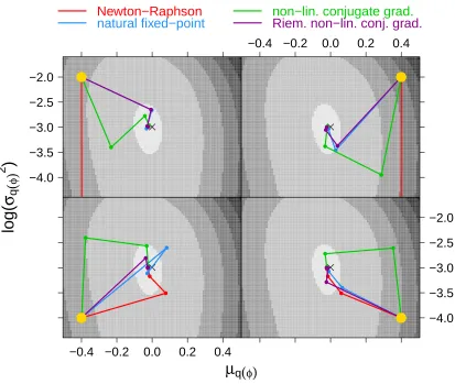
the Riemannian geometry adjustment involving the natural gradients given by (38). In most cases the iterations led to convergence to (µ∗_q(φ),(σ_q2_(φ))∗) and the first three iterates are plotted. However, Newton-Raphson failed to converge from the starting values in each of the upper panels and the subsequent iterates are outside of the image plot boundaries.

µ

(φ)

log(

σ

(

)

)

●

●

●

●

●

−0.4 −0.2 0.0 0.2 0.4

●

●

●

●

●

−0.4 −0.2 0.0 0.2 0.4

● ● ●

●

●

●

●

●

●

●

●

●

●

Newton−Raphson

natural fixed−point

non−lin. conjugate grad.

Riem. non−lin. conj. grad.

Figure 5: Iteration trajectories of four iterative algorithms aimed at solving the minimum Kullback-Leibler problem for a Gumbel random sample of size n = 20 with hy-perparameters µq(φ) = 0 and σq2(φ) = 1010. The initial value differs for each panel and is shown by the yellow dot. The iterative algorithms are: (1) Newton-Raphson fixed-point iteration based ongNR, (2) natural fixed-point iteration based

ongnat, (3) ordinary non-linear conjugate gradient method and (4) Riemannian