A Hierarchy of Support Vector Machines for Pattern Detection

A Hierarchy of Support Vector Machines for Pattern Detection

Hichem Sahbi [email protected]

Machine Intelligence Laboratory Department of Engineering University of Cambridge Trumpington Street Cambridge, CB2 1PZ, UK

Donald Geman [email protected]

Center for Imaging Science 302 Clark Hall

Johns Hopkins University 3400 N. Charles Street Baltimore, MD 21218, USA

Editor: Pietro Perona

Abstract

We introduce a computational design for pattern detection based on a tree-structured network of support vector machines (SVMs). An SVM is associated with each cell in a recursive partitioning of the space of patterns (hypotheses) into increasingly finer subsets. The hierarchy is traversed coarse-to-fine and each chain of positive responses from the root to a leaf constitutes a detection. Our objective is to design and build a network which balances overall error and computation.

Initially, SVMs are constructed for each cell with no constraints. This “free network” is then perturbed, cell by cell, into another network, which is “graded” in two ways: first, the number of support vectors of each SVM is reduced (by clustering) in order to adjust to a pre-determined, increasing function of cell depth; second, the decision boundaries are shifted to preserve all positive responses from the original set of training data. The limits on the numbers of clusters (virtual support vectors) result from minimizing the mean computational cost of collecting all detections subject to a bound on the expected number of false positives.

When applied to detecting faces in cluttered scenes, the patterns correspond to poses and the free network is already faster and more accurate than applying a single pose-specific SVM many times. The graded network promotes very rapid processing of background regions while maintain-ing the discriminatory power of the free network.

Keywords: statistical learning, hierarchy of classifiers, coarse-to-fine computation, support vector

machines, face detection

1. Introduction

cluttered backgrounds provides a running illustration of the ideas where the groupings are based on pose continuity.

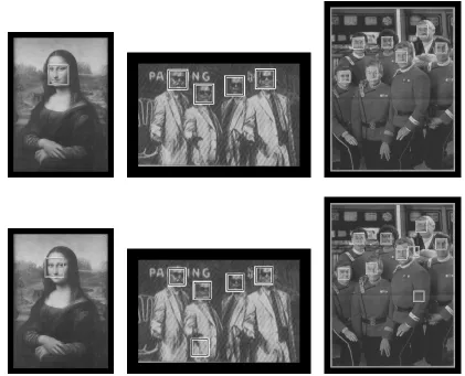
Our optimization framework is motivated by natural trade-offs among invariance, selectivity (background rejection rate) and the cost of processing the data in order to determine all detected patterns. In particular, it is motivated by the amount of computation involved when a single SVM, dedicated to a reference pattern (e.g., faces with a nearly fixed position, scale and tilt), is applied to many data transformations (e.g., translations, scalings and rotations). This is illustrated for face detection in Fig 1; a graded network of SVMs achieves approximately the same accuracy as a pattern-specific SVM but with order 100 to 1000 times fewer kernel evaluations, resulting from the network architecture as well as the reduced number of support vectors.

To design and construct such a graded network, we begin with a hierarchical representation of the space of patterns (e.g., poses of a face) in the form of a sequence of nested partitions, one for each level in a binary tree (Fleuret and Geman, 2001; Fleuret, 1999; Sahbi et al., 2002; Jung, 2001; Blanchard and Geman, 2005; Amit et al., 2004; Gangaputra and Geman, 2006a). Each cell - distin-guished subset of patterns - encodes a simpler, sub-classification task and is assigned a binary clas-sifier. The leaf cells represent the resolution at which we desire to “detect” the true pattern(s). There is also a “background class,” for example, a complex and heterogeneous set of non-distinguished patterns, which is statistically dominant (i.e., usually true). A pattern is “detected” if the classifier for every cell which covers it responds positively.

Initially, SVMs are constructed for each cell in the standard way (Boser et al., 1992) based on a kernel and training data – positive examples (from a given cell) and negative examples (“back-ground”). This is the “free network,” or “f-network”{ft}, where t denotes a node in the tree

hierar-chy. The “graded network,” or “g-network”{gt}, is indexed by the same hierarchy, but the number

of intervening terms in each gt is fixed in advance (by clustering those in ft as in Sch¨olkopf et al.,

1998), and grows with the level of t. (From here on, the vectors appearing gt will be referred to

as “support vectors” even though, technically, they are constructed from the actual support vectors

appearing in ft.) Moreover, the decision boundaries are shifted to preserve all positive responses

from the original set of training data; consequently, the false negative (missed detection) rate of gt

is at most that of ftand any pattern detected by the f-network is also detected by the g-network. But

the g-network will be far more efficient.

The limits on the numbers of support vectors result from solving a constrained optimization problem. We minimize the mean computation necessary to collect all detections subject to a

con-straint on the rate of false detections. (In the application to face detection, a false detection refers to

finding a face amidst clutter.) Mean computation is driven by the background distribution. This also involves a model for how the selectivity of an SVM depends on complexity, which is assumed pro-portional to the number of support vectors, and invariance, referring to the “scope” of the underlying cell in the hierarchy.

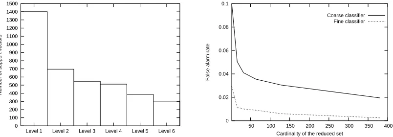
In the free network, the complexity of each SVM decision function depends in the usual way on the underlying probability distribution of the training data. For instance, the decision function for a linearly separable training set might be expressed with only two support vectors, whereas the SVMs induced from complex tasks in object recognition usually involve many support vectors (Osuna et al., 1997). For the f-network, the complexity generally decreases as a function of depth due to the progressive simplification of the underlying tasks. This is illustrated in Fig 2 (left) for

face detection; the classifiers ft were each trained on 8000 positive examples and 50,000 negative

Figure 1: Comparison between a single SVM (top row) dedicated to a nearly fixed pose and our designed network (bottom row) which investigates many poses simultaneously. The sizes

of the three images are, left to right, 520×739, 462×294 and 662×874 pixels. The

network achieves approximately the same accuracy as the pose-specific SVM but with order 100-1000 times fewer kernel evaluations. Some statistics comparing efficiency are given in Table 1.

Consider an SVM f in the f-network with N support vectors and dedicated to a particular hy-pothesis cell; this network is slow, but has high selectivity and few false negatives. The

correspond-ing SVM g has a specified number n of support vectors with n ≤ N. It is intuitively apparent that

g is less selective; this is the price for maintaining the false negative rate and reducing the number

of kernel evaluations. In particular, if n is very small, g will have low selectivity (cf. Fig 2 (right)). In general, of course, with no constraints, the fraction of support vectors provides a rough measure of the difficulty of the problem; here, however, we are artificially reducing the number of support vectors, thereby limiting the selectivity of the classifiers in the g-network.

Building expensive classifiers at the upper levels (n≈N) leads to intensive early processing,

Figures ”Mona Lisa” ”Singers” ”Star Trek” 1 SVM f-net g-net 1 SVM f-net g-net 1 SVM f-net g-net # Subimages Processed 2.105 _2.103 _2.103 _5.104 _8.102 _8.102 _2.105 _4.103 _4.103 # Kernel Evaluations 5.107 ₁₀7 _3.104 _2.107 _7.106 ₁₀4 _8.107 _2.107 _5.104 Processing Time (s) 172.45 28.82 0.53 55.87 17.83 0.26 270.1 48.92 0.87

# Raw Detections 3 3 4 12 14 15 19 20 20

Table 1: Comparisons among i) a single SVM dedicated to a small set of hypotheses (in this case a constrained pose domain), ii) the f-network and iii) our designed g-network, for the images

in Fig 1. For the single SVM, the position of the face is restricted to a 2×2 window, its

scale to the range [10,12]pixels and its orientation to [−50,+50_{]; the original image is}

downscaled 14 times by a factor of 0.83 and for each scale the SVM is applied to the

image data around each non-overlapping 2×2 block. In the case of the f and g-networks,

we use the coarse-to-fine hierarchy and the search strategy presented here.

0 100 200 300 400 500 600 700 800 900 1000 1100 1200 1300 1400 1500

Level 1 Level 2 Level 3 Level 4 Level 5 Level 6

Number of support vectors

0 0.02 0.04 0.06 0.08 0.1

50 100 150 200 250 300 350 400

False alarm rate

Cardinality of the reduced set Coarse classifier

Fine classifier

Figure 2: Left: The average number of support vectors for each level in an f-network built for face detection. The number of support vectors is decreasing due to progressive simplification of the original problem. Right: False alarm rate as a function of the number of support vectors using two SVM classifiers in the g-network with different pose constraints.

cost is also very large (cf. Fig 3, top rows). As an alternative to building the g-network, suppose we simply replace the SVMs in the upper levels of f-network with very simple classifiers (e.g., linear SVMs); then many background patterns will reach the lower levels, resulting in an overall loss of efficiency (cf. Fig 3, middle rows).

We focus in between these extremes and build{gt}to achieve a certain trade-off between cost

and selectivity (cf. Fig 3, bottom rows). Of course, we cannot explore all possible designs so a model-based approach is necessary: The false alarm rate of each SVM is assumed to vary with complexity and invariance in a certain way. This functional dependence is consistent with the one proposed in Blanchard and Geman (2005), where the computational cost of a classifier is modeled as the product of an increasing function of scope and an increasing function of selectivity.

Maximum Level Reached 1 2 3 4 5 6 # Samples 1697 56 4 1 0 2 (f-network)

# Samples 936 555 135 17 54 63 (heuristic)

# Samples 1402 336 2 0 3 17 (g-network)

# Kernel Evaluations 2−10 10−102 102−103 103−104 104−105 105−106 # Samples 0 0 0 1697 58 5

(f-network)

# Samples 936 755 67 2 0 0 (heuristic)

# Samples 1402 340 18 0 0 0 (g-network)

Figure 3: In order to illustrate varying trade-offs among cost, selectivity and invariance, and to demonstrate the utility of a principled, global analysis, we classified 1760 subimages of

size 64×64 extracted from the image shown above using three different types of SVM

scene parsing. For some problems, dedicating a single classifier to each hypothesis, or a cascade (linear chain) of classifiers to a small subset of hypotheses (see Section 2), and then training with existing methodology (even off-the-shelf software) might suffice, in fact provide state-of-the-art performance. This seems to the case for example with frontal face detection as long as large training sets are available, at least thousands of faces and sometimes billions of negative examples, for learning long, powerful cascades. However, those approaches are either very costly (see above) or may not scale to more ambitious problems involving limited data, or more complex and varied interpretations, because they rely too heavily on brute-force learning and lack the structure necessary to hardwire efficiency by simultaneously exploring multiple hypotheses.

We believe that hierarchies of classifiers provide such a structure. In the case of SVMs, which may require extensive computation, we demonstrate that building such a hierarchy with a global design which accounts for both cost and error is superior to either a single classifier applied a great many times (a form of template-matching) or a hierarchy of classifiers constructed independently, node-by-node, without regard to overall performance. We suspect that the same demonstration could be carried out with other “base classifiers” as long as there is a natural method for adjusting the amount of computation; in fact, the global optimization framework could be applied to improve other parsing strategies, such as cascades.

The remaining sections are organized as follows: A review of coarse-to-fine object detection, including related work on cascades, is presented in Section 2. In Section 3, we discuss hierarchical representation and search in general terms; decomposing the pose space provides a running exam-ple of the ideas and sets the stage for our main application - face detection. The f-network and g-network are defined in Section 4, again in general terms and the statistical framework and op-timization problem are laid out in Section 5. This is followed in Section 6 by a new formulation of the “reduced set” method (Burges, 1996; Sch ¨olkopf et al., 1998), which is used to construct an SVM of specified complexity. These ideas are illustrated for a pose hierarchy in Section 7, includ-ing a specific instance of the model for chain probabilities and the correspondinclud-ing minimization of cost subject to a constraint on false alarms. Experiments are provided in Section 8, where the g-network is applied to detect faces in standard test data, allowing us to compare our results with other methods. Finally, some conclusions are drawn in Section 9.

2. Coarse-to-Fine Object Detection

Our work is motivated by difficulties encountered in inducing semantic descriptions of natural scenes from image data. This is often computationally intensive due to the large amount of data to be processed with high precision. Object detection is such an example and has been widely investigated in computer vision; see for instance Osuna et al. (1997); Fleuret and Geman (2001); Kanade (1977); Schneiderman and Kanade (2000); Sung (1996); Viola and Jones (2001) for work on face detection. Nonetheless, there is as yet no system which matches human accuracy; moreover, the precision which is achieved often comes at the expense of run-time performance or a reliance on massive training sets.

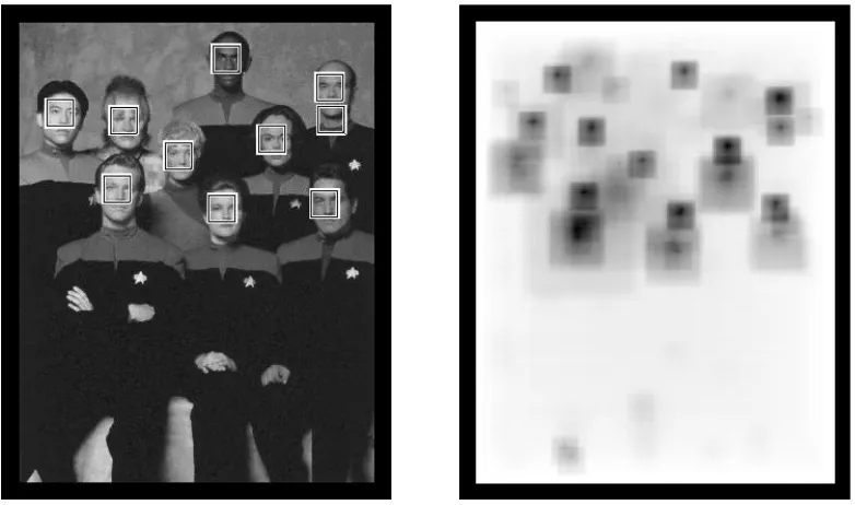
Figure 4: Left: Detections using our system. Right: The darkness of a pixel is proportional to the amount of local processing necessary to collect all detections.

other tasks such as compression, registration, noise reduction and estimating motion and binocular disparity. In the case of object detection, one strategy is to focus rapidly on areas of interest by finding characteristics which are common to many instantiations; in particular, background regions are quickly rejected as candidates for further processing (see Fig 4).

In the context of finding faces in cluttered scenes, Fleuret and Geman (2001) developed a fast, coarse-to-fine detector based on simple edge configurations and a hierarchical decomposition of the space of poses (location, scale and tilt). (Similar, tree-structured recognition strategies appear in Geman et al. (1995); Baker and Nayar (1996).) One constructs a family of classifiers, one for each cell in a recursive partitioning of the pose space and trained on a sub-population of faces meeting the pose constraints. A face is declared with pose in a leaf cell if all the classifiers along the chain from root to leaf respond positively. In general, simple and uniform structures in the scene are quickly rejected as face locations (i.e., very few classifiers are executed before all possible complete chains are eliminated) whereas more complex regions, for instance textured areas and face-like structures, require deeper penetration into the hierarchy. Consequently, the overall cost to process a scene is dramatically lower than looping over many individual poses, a form of template- matching (cf. Fig 1).

et al. (2005); Romdhani et al. (2001) for face detection, and the cascade of inner products in Keren et al. (2001) for object identification, employ very simple linear classifiers. In nearly all cases the individual node learning problems are treated heuristically; an exception is Wu et al. (2005), where, for each node, the classifiers are designed to solve a (local) optimization problem constrained by desired (local) error rates.

There are several important differences between our work and cascades. Cascades are coarse-to-fine in the sense of background filtering whereas our approach is coarse-coarse-to-fine both in the sense of hierarchical pruning of the background class and representation of the space of hypotheses. In particular, cascades operate in a more or less brute-force fashion because every pose (e.g., position, scale and tilt) must be examined separately. In comparing the two strategies, especially our work with cascades of SVMs for face detection as in Kienzle et al. (2004); Romdhani et al. (2001), there is then a trade-off between very fast early rejection of individual hypotheses (cascades) and somewhat slower rejection of collections of hypotheses (tree-structured pruning).

No systematic comparison with cascades has been attempted. Moving beyond an empirical study would require a model for how cost scales with other factors, such as scope and selectivity. One such model was proposed in Blanchard and Geman (2005), in which the computational cost

C(f)of a binary classifier f dedicated to a set A of hypotheses (against a universal “background”

alternative) is expressed as

C(f) =Γ(|A|)×Ψ(1−δ)

whereδis false positive rate of the classifier f (so 1−δis what we have called the selectivity) and

ΓandΨare increasing functions withΓsubadditive andΨconvex. (Some empirical justification

for this model can be found in Blanchard and Geman (2005).) One can then compare the cost of testing a “small” set A of hypotheses (e.g., all poses over a small range of locations, scales and tilts,

as in cascades) versus a “large” set B⊃A (e.g., many poses simultaneously, as here). Under this

cost model, and equalizing the selectivity, the subadditivity ofΓwould render the test dedicated to

B cheaper than doing the test dedicated to A approximately |_|A_B|_| times, even ignoring the inevitable reduction in selectivity due to repeated tests.

More importantly, perhaps, it is not clear that cascades will scale to more ambitious problems involving many classes and instantiations since repeatedly testing a coarse set of hypotheses will lack selectivity and repeatedly testing a narrow one will require a great many implementations.

Finally, to our knowledge, the work presented in this paper is the first to consider a global construction of the system in an optimization framework. In particular, no global criteria appear in either Fleuret and Geman (2001) or Viola and Jones (2001); in the former, the edge-based classifiers are of roughly constant complexity whereas in the latter the complexity of the classifiers along the cascade is not explicitly controlled.

3. Hierarchical Representation and Search

LetΛdenote a set of “patterns” or “hypotheses” of interest. Our objective is to determine which,

if any, of the hypothesesλ∈Λis true, the alternative being a statistically dominant “background”

hypothesis{0}, meaning that most of the time 0 is the true explanation. Let Y denote the true state;

Y =0 denotes the background state. Instead of searching separately for each λ∈Λ, consider a

coarse-to-fine search strategy in which we first try to exploit common properties (“shared features”)

of all hypotheses to “test” simultaneously for allλ∈Λ, that is, test the compound hypothesis H :

the test is positive, we separately test two disjoint subsets ofΛagainst H0; and so forth in a nested

fashion.

The tests are constructed to be very conservative in the sense that each false negative error rate

is very small, that is, given that Y ∈A, we are very unlikely to declare background if A⊂Λis the

subset of hypotheses tested at a given stage. The price for this small false negative error is of course a non-negligible false positive error, particularly for testing “large” subsets A. However, this proce-dure is highly efficient, particularly under the background hypothesis. This “divide-and-conquer” search strategy has been extensively examined, both algorithmically (see for example Fleuret and Geman, 2001; Amit et al., 2004; Gangaputra and Geman, 2006a) and mathematically (Blanchard and Geman, 2005; Fleuret, 1999; Jung, 2001).

Note: There is an alternate formulation in which Y is directly modeled as a subset ofΛwith Y = /0 corresponding to the background state. In this case, at each node of the hierarchy, we are testing a hypothesis of the form H : Y∩A6= /0vs the alternative Y∩A=/0. In practice, the two formulations are essentially equivalent; for instance, in face detection, we can either “decompose” a set of “ref-erence” poses which can represent at most one face and then execute the hierarchical search over subimages or collect all poses into one hierarchy with virtual tests near the root; see Section 7.1.

We shall adopt the simpler formulation in which Y ∈Λ∪ {0}.

Of course in practice we do all the splitting and construct all the “tests” in advance. (It should be emphasized that we are not constructing a decision tree; in particular, we are recursively partitioning the space of interpretations not features and, when the hierarchy is processed, a data point can travel down many branches and arrive at none of the leaves.) Then, on line, we need only execute the tests in the resulting hierarchy coarse-to-fine. Moreover, the tests are simply standard classifiers induced

from training data - examples of Y∈A for various subsets of A and examples of Y=0. In particular,

in the case of object detection, the classifiers are constructed from the usual types of image features, such as averages, edges and wavelets (Sahbi et al., 2002).

The nested partitions are naturally identified with a tree T . There is a subsetΛt for each node

t of T , including the root (Λroot =Λ) and each leaf t∈∂T . We will write t= (l,k)to denote the k’th node of T at depth or level l. For example, in the case of a binary tree T with L levels, we then

have:







Λ_1,1 = Λ

Λ_l,k = Λ_l+1,2k−1 ∪ Λ_l+1,2k

Λ_l+1,2k−1 ∩ Λ_l+1,2k=/0

l∈ {1, ...,L−1}, k∈

1, ...,2l−1 .

The hierarchy can be manually constructed (as here, copying the one in Fleuret and Geman, 2001) or, ideally, learned.

Notice that the leaf cellsΛt,t∈∂T , needn’t correspond to individual hypotheses. Instead, they

represent the finest “resolution” at which we wish to estimate Y . More careful disambiguation among candidate hypotheses may require more intense processing, perhaps involving online opti-mization. It then makes sense to modify our definition of Y to reflect this possible coarsening of the original classification problem: the possible “class” values are then{0,1, ...,2L−1}, corresponding to “background” ({0}) and the 2L−1“fine” cells at the leaves of the hierarchy.

Example: The Hierarchy for Face Detection. Here, the pose of an object refers to parameters

(p,φ,s)∈R4 _{: p∈[−8,+8]}2_,φ∈[−200_,+200_{],s∈[10,20]}

(p,φ,s)∈R4 _{: p∈[−1,+1]}2_,φ∈[00_,+200_{],s∈[15,20]}

Figure 5: An illustration of the pose hierarchy showing a sample of faces at the root cell and at one of the leaves.

one object class – faces – the family of hypotheses of interest is a set of posesΛ. Specifically, we

focus attention on the position, tilt and scale of a face, denotedθ= (p,φ,s), where p is the midpoint

between the eyes, s is the distance between the eyes andφis the angle with the line orthogonal to

the segment joining the eyes. We then define

Λ=

(p,φ,s)∈R4 : p∈[−8,+8]2,φ∈[−200,+200],s∈[10,20] .

Thus, we regardΛas a “reference set” of poses in the sense of possible instantiations of a single

face within a given 64×64 image assuming that the position is restricted to a subwindow (e.g., an

16×16 centered in the subimage) and the scale to the stated range. The “background hypothesis”

is “no face” (with pose in Λ). The leaves of T do not correspond to individual posesθ∈Λ; for

instance, the final resolution on position is a 2×2 window. Hence, each “object hypothesis” is a

small collection of fine poses.

The specific hierarchy used in our experiments is illustrated in Fig (5). It has six levels(L=6),

corresponding to three quaternary splits in location (four 8×8 blocks, etc.) and one binary split

both on tilt and scale. Therefore, writingνlfor the number of cells in T at depth l:ν1=1,ν2=41,

ν3=42=16,ν4=43=64,ν5=2 43=128 andν6=2243=256.

This is the same, manually-designed, pose hierarchy that was used in Fleuret and Geman (2001). The partitioning based on individual components, as well as the splitting order, is entirely ad hoc. The important issue of how to automatically design or learn the “divide-and-conquer” architecture is not considered here. Very recent work on this topic appears in Fan (2006) and Gangaputra and Geman (2006a).

Search Strategy:

Consider coarse-to-fine search in more detail. Let Xt be the test or classifier associated with

of H0: Y =0. Also, letω∈Ωrepresent the underlying data or “pattern” upon which the tests are

based; hence the true class ofωis Y(ω)and Xt :Ω−→ {0,1}.

The result of coarse-to-fine search applied toωis a subset D(ω)⊂Λof “detections”, possibly

empty, defined to be allλ∈Λfor which Xt(ω) =1 for every test which “covers”λ, that is, for which

λ∈Λt. Equivalently, D is the union over allΛt,t∈∂T such that Xt =1 and the test corresponding to every ancestor of t∈∂T is positive, that is, all “complete chains of ones” (cf. Fig 6, B).

Both breadth-first and depth-first coarse-to-fine search lead to the same set D. Breadth-first search is illustrated in Fig (6, C): Perform X1,1; if X1,1=0, stop and declare D= /0; if X1,1 =1,

perform both X2,1 and X2,2 and stop only if both are negative; etc. Depth-first search explores the

sub-hierarchy rooted at a node t before exploring the brother of t. In other words, if Xt=1, we visit recursively the sub-hierarchies rooted at t; if Xt =0 we “cancel” all the tests in this sub-hierarchy.

In both cases, a test is performed if and only if all its ancestors are performed and are positive.

(These strategies are not the same if our objective is only to determine whether or not D= /0; see

the analysis in Jung (2001).)

Notice that D= /0 if and only if there is a “null covering” of the hierarchy in the sense of a

collection of negative responses whose corresponding cells cover all hypotheses inΛ. The search

is terminated upon finding such a null covering. Thus, for example, if X1,1=0, the search is

ter-minated as there cannot be a complete chain of ones; similarly, if X2,1=0 and X3,3=X3,4=0, the

search is terminated.

(A) (B) (C)

θ3 θ4

Figure 6: A hierarchy with fifteen tests. (A) The response to an input image were all the tests to be performed; the positive tests are shown in black and negative tests in white. (B) There are two complete chains of ones; in the case of object detection, the detected pose is the average over those in the two corresponding leaves. (C) The breadth-first search strategy with the executed tests are shown in color; notice that only seven of the tests would actually be performed.

Example: The Search Strategy for Face Detection. Images ω are encoded using a vector of wavelet coefficients; in the remainder of this paper we will write x to denote this vector of coeffi-cients computed on a given 64×64 subimage. If D(x)6=/0, the estimated pose of the face detected

inωis obtained by averaging over the “pose prototypes” of each leaf cell represented in D, where

the pose prototype ofΛt is the midpoint (cf. Fig 6, B).

A scene is processed by visiting non-overlapping 16×16 blocks, processing the surrounding

Figure 7: Multi-scale search. The original image (on the left) is downscaled three times. For each

scale, the base face detector visits each non-overlapping 16×16 block, and searches the

surrounding image data for all faces with position in the block, scale anywhere in the range[10,20]and in-plane orientation in the range[−20o,+20o_].

search strategy described earlier in this section. This process makes it possible to detect all faces whose scale s lies in the interval [10,20]and whose tilt belongs to[−20o,+20o_{]. Faces at scales}

[20,160]are detected by repeated down-sampling (by a factor of 2) of the original image, once for

scales[20,40], twice for[40,80]and thrice for[80,160](cf. Fig 7). Hence, due to high invariance to scale in the base detector, only four scales need to be investigated altogether.

Alternatively, we can think of an extended hierarchy over all possible poses, with initial branch-ing into disjoint 16×16 blocks and disjoint scale ranges, and with virtual tests in the first two layers which are passed by all inputs. Given color or motion information (Sahbi and Boujemaa, 2000), it

might be possible to design a test which handles a set of poses larger thanΛ; however, our test at

the root (accounting simultaneously for all poses inΛ) is already quite coarse.

4. Two SVM Hierarchies

Suppose we have a training set

T

ωis some 64×64 subimage taken, for example, from the Web, and either belongs to the “object

examples”

L

B

Y(ω) =0).

All tests Xt,t∈T , are based on SVMs. We build one hierarchy, the free network or f-network for

4.1 The f-network

Let ft be an SVM dedicated to separating examples of Y ∈Λt from examples of Y =0. (In our

ap-plication to face detection, we train ft based on face imagesωwith pose inΛt.) The corresponding

test is simply 1{ft>0}. We refer to{ft,t∈T}as the f-network. In practice, the number of support vectors decreases with the depth in the hierarchy since the classification tasks are increasingly

sim-plified; see Fig 2, left. We assume the false negative rate of ft is very small for each t; in other

words, ft(ω)>0 for nearly all patternsωfor which Y(ω)∈Λt. Finally, denote the corresponding

data-dependent set of detections of the f-network by Df.

4.2 The g-network

The g-network is based on the same hierarchy{Λt} as the f-network. However, for each cellΛt,

a simplified SVM decision function gt is built by reducing the complexity of the corresponding

classifier ft. The set of hypotheses detected by the g-network is denoted by Dg. The targeted

complexity of gt is determined by solving a constrained minimization problem (cf. Section 5).

We want gt to be both efficient and respect the constraint of a negligible false negative rate.

As a result, for nodes t near the root of T the false positive rate of gt will be higher than that of

the corresponding ft since low cost comes at the expense of a weakened background filter. Put

differently, we are willing to sacrifice selectivity for efficiency, but not at the expense of missing (many) instances of our targeted hypotheses. Thus, for both networks, a positive test by no means signals the presence of a targeted hypothesis, especially for the very computationally efficient tests in the g-network near the top of the hierarchy.

Instead of imposing an absolute constraint on the false negative error, we impose one relative to

the f-network, referred to as the conservation hypothesis: For each t∈T andω∈Ω:

ft(ω)>0⇒gt(ω)>0.

This implies that an hypothesis detected by the f-network is also detected by the g-network, namely

Df(ω)⊂Dg(ω), ∀ω∈Ω.

Consider two classifiers gt and gs in the g-network and suppose node s is deeper than node t.

With the same number of support vectors, gt will generally produce more false alarms than gssince

more invariance is expected of gt (cf. Fig 2, right). In constructing the g-network, all classifiers

at the same level will have the same number of support vectors and are then expected to have approximately the same false alarm rate (cf. Fig 8).

In the following sections, we will introduce a model which accounts for both the overall mean cost and the false alarm rate. This model is inspired by the trade-offs among selectivity, cost and invariance discussed above. The proposed analysis is performed under the assumption that there exists a convex function which models the false alarm rate as a function of the number of support vectors and the degree of “pose invariance”.

5. Designing the g-network

Let P be a probability distribution onΩ. Write Ω=

L

B

L

0 0.01 0.02 0.03 0.04 0.05 0.06 0.07

0 20 40 60 80 100 120 140

False alarm rate

Cardinality of the reduced set Level 1 Level 5 Level 6-1 Level 6-2 Level 6-3

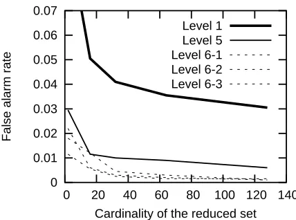
Figure 8: For the root cell, a particular cell in the fifth level and three particular pose cells in the sixth level of the g-network, we built SVMs with varying numbers of (virtual) support vectors. All curves show false alarm rates with respect to the number of (virtual) support vectors. For the sixth level, and in the regime of fewer than 10 (virtual) support vectors, the false alarm rates show considerable variation, but have the same order of magnitude. These experiments were run on background patterns taken from 200 images including highly textured areas (flowers, houses, trees, etc.)

contains all the background patterns. Define P0(.) =P(.|Y =0) and P1(.) =P(.|Y >0), the

con-ditional probability distributions on background and object patterns, respectively. Throughout this paper, we assume that P(Y=0)>>P(Y>0), which means that the presence of the targeted pattern is considered to be a rare event in data sampled under P.

Face Detection Example (cont): We might take P to be the empirical distribution on a huge set

of 64×64 subimages taken from the Web. Notice that, given a subimage selected at random, the

probability to have a face present with location near the center is very small.

Relative to the problem of deciding Y =0 vs Y 6=0, that is, deciding between “background”

and “object” (some hypothesis inΛ), the two error rates for the f-network are P0(Df 6=/0), the false

positive rate, and P1(Df =/0), the false negative rate. The total error rate is, P0(Df 6=/0)P(Y =0) + P1(Df =/0) P(Y >0). Clearly this total error is largely dominated by the false alarm rate.

Recall that for each node t∈T there is a subsetΛt of hypotheses and an SVM classifier gt with

nt support vectors. The corresponding test for checking Y ∈Λt against the background alternative

is 1{gt>0}. Our objective is to provide an optimization framework for specifying{nt}.

5.1 Statistical Model

We now introduce a statistical model for the behavior of the g-network. Consider the event that a

background pattern traverses the hierarchy up to node t, namely the event T

s∈At{gs>0}, where

assume that the probability of this event under P0, namely

P0(gs>0,s∈

A

depends only on the level of t in the hierarchy (and not on the particular set

A

numbers n1, ...,nl−1 of support vectors at levels one through l−1, where t is at level l. These

assumptions are reasonable and roughly satisfied in practice; see Sahbi (2003).

The probability in (1) that a background pattern reaches depth l, that is, there is a chain of

positive responses of length l−1, is then denoted by δ(l−1; n), where n denotes the sequence

(n1, ...,nL). Naturally, we assume thatδ(l; n)is decreasing in l. In addition, it is natural to assume

thatδ(l; n)is a decreasing function of each nj,1≤ j≤l. In Section 7 we will present an example

of a two-dimensional parametric family of such models.

There is an equivalent, and useful, reformulation of these joint statistics in terms of conditional

false alarm rates (or conditional selectivity). One specifies a model by prescribing the quantities

P0(groot >0), P0(gt>0|gs>0,s∈

A

for all nodes t with 2≤l(t)≤L. Clearly, the probabilities in (1) determine those in (2) and

vice-versa.

Note: We are not specifying a probability distribution on the entire family of variables{gt,t∈T},

equivalently, on all labeled trees. However, it can be shown that any (decreasing) sequence of positive numbers p1, ...,pLfor the chain probabilities is “consistent” in the sense of providing a

well-defined distribution on traces, the labeled subtrees that can result from coarse-to-fine processing, which necessarily are labeled “1” at all internal nodes; see Gangaputra and Geman (2006b).

In order to achieve efficient computation (at the expense of extra false alarms relative to the

f-network), we choose n= (n1, ...,nL) to solve a constrained minimization problem based on the

mean total computation in evaluating the g-network and a bound on the expected number of detected background patterns:

min

n

C

(3)

where E0refers to expectation with respect to the probability measure P0. We first compute this

ex-pected cost, then consider the constraint in more detail and finally turn to the problem of choosing the model.

Note: In our formulation, we are assuming that overall average computation is well-approximated

5.2 Cost of the g-network

Let ct indicate the cost of performing gt and assume

ct=a nt+b.

Here a represents the cost of kernel evaluation and b represents the cost of “preprocessing” – mainly

extracting features from a patternω(e.g., computing wavelet coefficients in a subimage). We will

also assume that all SVMs at the same level of the hierarchy have the same number of support vectors, and hence approximately the same cost.

Recall thatνl is the number of nodes in T at level l; for example, for a binary tree,νl =2l−1.

The global cost is then:

Cost =

∑

t

1_{g

t is performed}ct

=

L

∑

νl

∑

1_{g

l,kis performed}cl,k

(4)

since gt is performed in the coarse-to-fine strategy if and only if gs>0∀s∈

A

equation (4), withδ(0; n) =1,

C

=

L

∑

νl

∑

P0({gl,k is performed}) cl,k

=

L

∑

νl

∑

δ(l−1; n)cl,k

=

L

∑

νlδ(l−1; n)cl

= a L

∑

νlδ(l−1; n)nl+b L

∑

νl δ(l−1; n).

The first term is the SVM cost and the second term is the total preprocessing cost. In the application to face detection we shall assume the preprocessing cost – the computation of Haar

wavelet coefficients for a given subimage – is small compared with kernel evaluations, and set a=1

and b=0. Hence,

C

∑

νl nl δ(l−1; n).

5.3 Penalty for False Detections

Recall that Dg(ω)– the set of detections – is the union of the setsΛt over all terminal nodes t for

which there is a complete chain of positive responses from the root to t. For simplicity, we assume that|Λt|is the same for all terminal nodes t. Hence |Dg| is proportional to the total number of

complete chains:

|Dg|∝

∑

1{gt>0}

∏

s∈At

It follows that

E0|Dg| ∝ E0

∑

1{gt>0}

∏

s∈At 1{gs>0}

=

∑

t∈∂T

δ(L; n)

= νLδ(L; n)

By the Markov inequality,

P0(Dg6=/0) =P0(|Dg| ≥1)≤E0|Dg|.

Hence bounding the mean size of Dg also yields the same bound on the false positive probability.

However, we cannot calculate P0(|Dg| ≥1)based only on our model{δ(l; n)}l since this would

re-quire computing the probability of a union of events and hence a model for the dependency structure

among chains.

Finally, since we are going to use the SVMs in the f-network to build those in the g-network,

the number of support vectors nl for each SVM in the g-network at level l is bounded by the

corre-sponding number, Nl, for the f-network. (Here, for simplicity, we assume that Ntis roughly constant

in each level; otherwise we take the minimum over the level.) Summarizing, our constrained optimization problem (3) becomes

min

n1,...,nL

n1+

L

∑

νl nlδ(l−1; n) s.t.

ν

Lδ(L; n) ≤ µ

0 < nl ≤ Nl. (5)

5.4 Choice of Model

In practice, one usually stipulates a parametric family of statistical models (in our case the chain probabilities) and estimates the parameters from data. Let{δ(l; n,β)},β∈B}denote such a family whereβdenotes a parameter vector, and let n∗=n∗(β)denote the solution of (5) for modelβ. We

propose to chooseβby comparing population and empirical statistics. For example, we might select

the model for which the chain probabilities best match the corresponding relative frequencies when

the g-network is constructed with n∗(β)and run on sample background data. Or, we might simply

compare predicted and observed numbers of background detections:

β∗₌. _{arg min}

β∈B|E0(|Dg|; n

∗_(β))−ˆµ

0(n∗(β))|

where ˆµ0(n∗(β))is the average number of detections observed with the g-network constructed from n∗(β). In Section 7 we provide a concrete example of this model estimation procedure.

6. Building the g-network

Since the construction is node-by-node, we can assume throughout this section that t is fixed and

thatΛ=Λt and f = ft are given, where f is an SVM with Nf support vectors. Our objective is to

build an SVM g=gt with two properties:

• g is to have Ng<Nf support vectors, where Ng=n∗_l(t) and n∗= (n∗1, ...,n∗L) is the optimal

• The “conservation hypothesis” is satisfied; roughly speaking this means that detections under

f are preserved under g.

Let x(ω)∈_Rq _{be the feature vector; for simplicity, we suppress the dependence on}ω_{. The}

SVM f is constructed as usual based on a kernel K which implicitly defines a mappingΦ from

the input space Rq into a high-dimensional Hilbert space

H

Support vector training (Boser et al., 1992) builds a maximum margin hyperplane (wf,bf) in

H

Re-ordering the training set as necessary, let Φ(v(1)), ...,Φ(v(Nf)_{) and{}α

1, ...,αNf}denote,

re-spectively, the support vectors and the training parameters. The normal wf of the hyperplane is

wf = ∑ Nf

i=1 αiy(i)Φ(v(i)).

The decision function inRqis non-linear:

f(x) =hwf,Φ(x)i + bf = Nf

∑

αiy(i)K(v(i),x) + bf.

The parameters{αi}and bf can be adjusted to ensure thatkwfk2=1.

The objective now is to determine(wg,bg), where

g(x) = hwg,Φ(x)i + bg = Ng

∑

γkK(z(k),x) + bg.

Here

Z

z(1), ...,z(Ng) _{is the reduced set of support vectors (cf. Fig 9, right),}γ₌γ

1, ...,γNg the underlying weights, and the labels y(k)have been absorbed intoγ.

0 0.2 0.4 0.6 0.8 1

10 20 30 40 50 60 70 80 90 100

Correlation

Reduction factor (%) Clustering for initialization Random initialization

faces non−faces

Figure 9: Left: The correlation is illustrated with respect to the reduction factor (Ng

Nf ×100). These

experiments are performed on a root SVM classifier using the Gaussian kernel (σis set

6.1 Determining wg: Reduced Set Technique

The method we use is a modification of the reduced set technique (RST) (Burges, 1996; Burges and Sch¨olkopf, 1997). Choose the new normal vector to satisfy:

w∗_g=arg min

wg:kwgk=1

hwg−wf,wg−wfi.

Using the kernel trick, and since wg=∑

Ng

k=1γkΦ(z(k)), the new optimization problem becomes:

min

Z,γ

∑

(k)_,z(l)_{) +}

∑

i,j

αiαj y(i)y(j)K(v(i),v(j))−2

∑

γkαi y(i)K(z(k),v(i)). (6)

For some kernels (for instance the Gaussian), the function to be minimized is not convex; con-sequently, with standard optimization techniques such as conjugate gradient, the normal vector resulting from the final solution(

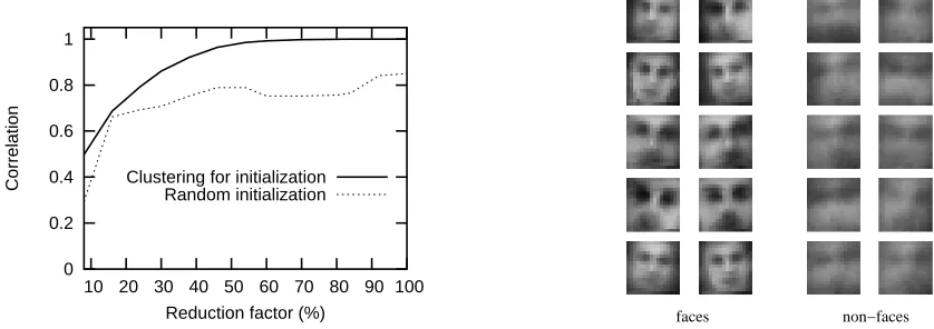
Z

prob-lem was analyzed in Sahbi (2003), where it is shown that, in the context of face detection, a good initialization of the minimization process can be obtained as follows: First cluster the initial set of support vectors {Φ(v(1)), ...,Φ(v(Nf)_{)}, resulting in N}

g centroids, each of which then represents a

dense distribution of the original support vectors. Next, each centroid, which is expressed as a linear combination of original support vectors, is replaced by one support vector which best approximates this linear combination. Finally, this new reduced set is used to initialize the search in (6) in order to improve the final solution. Details may be found in Sahbi (2003) and the whole process is illustrated in Section 7.

6.2 Determining bg: Conservation Hypothesis

Regardless of how bg is selected, g is clearly less powerful than f . However, in the hierarchical

framework, particularly near the root, the two types of mistakes (namely not detecting patterns in

Λand detecting background) are not equally problematic. Once a distinguished pattern is rejected

from the hierarchy it is lost forever. Hence we prefer to severely limit the number of missed de-tections at the expense of additional false positives; hopefully these background patterns will be filtered out before reaching the leaves.

We make the assumption that the classifiers in the f-network have a very low false negative rate. Ideally, we would choose bg such that g(x(ω))>0 for everyω∈Ωfor which f(x(ω))>0.

However, this results in an unacceptably high false positive rate. Alternatively, we seek to minimize

P0(g ≥ 0| f < 0)

subject to

P1(g < 0| f ≥0)≤ε.

Since we do not know the joint law of(f,g)under either P0or P1, these probabilities are estimated

empirically: for each bg calculate the conditional relative frequencies using the training data and

then choose the optimal bgbased on these estimates.

7. Application to Face Detection

include artificial neural networks (Schneiderman and Kanade, 2000; Sung, 1996; Rowley et al., 1998; F´eraud et al., 2001; Garcia and Delakis, 2004), networks of linear units (Yang et al., 2000), support vector machines (Osuna et al., 1997; Evgeniou et al., 2000; Heisele et al., 2001; Romdhani et al., 2001; Kienzle et al., 2004), Bayesian inference (Cootes et al., 2000), deformable templates (Miao et al., 1999), graph-matching (Leung et al., 1995), skin color learning (Hsu et al., 2001; Sahbi and Boujemaa, 2000), and more rapid techniques such as boosting a cascade of classifiers (Viola and Jones, 2001; Li and Zhang, 2004; Wu et al., 2005; Socolinsky et al., 2003; Elad et al., 2002) and hierarchical coarse-to-fine processing (Fleuret and Geman, 2001).

The face hierarchy was described in Section 3. We now introduce a specific model for (1), the probability of a chain under the background hypothesis, and finally the solution to the resulting instance of the constrained optimization problem expressed in (8) below. The probability model links the cost of the SVMs to their underlying level of invariance and selectivity. Afterwords, in Section 8, we illustrate the performance of the designed g-network in terms of speed and error on both simple and challenging face databases including the CMU and the MIT datasets.

7.1 Chain Model

Our model family is{δ(l; n,β),β∈B}, where δ(l; n,β)is the probability of a chain of “ones” of

depth l−1. These probabilities are determined by the conditional probabilities in (2). Denote these

by

δ(1; n,β) =P0(groot >0)

and

δ(l|1, ...,l−1; n,β) =P0(gt>0|gs>0,s∈

A

Specifically, we take:

δ(1; n,β) = _β1

1n1 β1>0

δ(l|1, ...,l−1; n,β) = _β β1n1+...+βl−1nl−1

1n1+...+βl−1nl−1+βlnl , β1, ...,βl>0.

Loosely speaking, the coefficientsβ={βj j=1, ...,L}are inversely proportional to the degree

of “pose invariance” expected from the SVMs at different levels. At the upper, highly invariant,

levels l of the g-network, minimizing computation yields relatively small values ofβland vice-versa

at the lower, pose-dedicated, levels. The motivation for this functional form is that the conditional false alarm rate δ(l | 1, ...,l−1; n,β) should be increasing as the number of support vectors in

the upstream levels 1, ...,l−1 increases. Indeed, when gs>0 for all nodes s upstream of node

t, and when these SVMs have a large number of support vectors and hence are very selective, the

background patterns reaching node t resemble faces very closely and are likely to be accepted by the test at t. Of course, fixing the numbers of support vectors upstream, the conditional selectivity (that is, one minus the false positive error rate) at level l grows with nl. Notice also that the model does not anticipate exponential decay, corresponding to independent tests (under P0) along the branches of the hierarchy.

Using the marginal and the conditional probabilities expressed above, the probabilityδ(l; n,β) to have a chain of ones from the root cell to any particular cell at level l is easily computed:

δ(l; n,β) = 1 β1n1

β1n1

β1n1+β2n2

...β1n1+...+βl−1nl−1

=

l

∑

βjnj

!−1

. (7)

Clearly, for any n andβ, these probabilities decrease as l increases.

7.2 The Optimization Problem

Using (7), the constrained minimization problem (5) becomes:

min

n1,...,nL 

n1 +

L

∑

l−1

∑

βini

!−1

νl nl

  s.t.      νL L

∑

βini

!−1

≤ µ

0 < nl ≤ Nl.

(8)

This problem is solved in two steps:

• Step I: Start with the solution for a binary network (i.e.,νl+1=2νl). This solution is provided

in Appendix A.

• Step II: Pass to a dyadic network using the solution to the binary network, as shown in Sahbi

(2003, p. 127).

7.3 Model Selection

We use a simple function with two degrees of freedom to characterize the growth ofβ1, ...,βL:

βl =Ψ−₁1 exp{Ψ2(l−1)} (9)

whereΨ= (Ψ1,Ψ2)are positive. HereΨ1represents the degree of pose invariance at the root cell

andΨ2is the rate of the decrease of this invariance. Let n∗(Ψ)denote the solution to (8) forβgiven

by (9) and suppose we restrictΨ∈Q, a discrete set. (In our experiments,|Q|=100 corresponding

to ten choices for each parameterΨ1andΨ2, namelyΨ1ranges from 0.0125 to 0.2 andΨ2ranges

from 0.1 to 1.0, both in equal steps.) In other words, n∗(Ψ) are the optimal numbers of support vectors found when minimizing total computation (8) under the false positive constraint for a given fixedβ={β1, ...,βL}determined by (9). ThenΨ∗is selected to minimize the discrepancy between

the model and empirical conditional false positive rates:

min Ψ∈Q

L

∑

δ(l|1, ...,l−1; n

∗_{(Ψ),Ψ)−δˆ(l|1, ...,l−1; n}∗_(Ψ))

(10)

where ˆδ(l|1, ...,l−1; n∗(Ψ))is the underlying empirical probability of observing gt >0 given that gs>0 for all ancestors s of t, averaged over all nodes t at level l, when the g-network is built with

n∗(Ψ)support vectors.

Algorithm: Design of the g-network.

- Build the f-network using standard SVM training and learning set

L

B

- for(Ψ1,Ψ2)∈Q do

-βl ← Ψ−11 exp{Ψ2(l−1)}, l=1, ...,L

- Compute n∗(Ψ)using (8).

- Build the g-network using the reduced set method and the specified costs n∗(β).

- Compute the model and empirical conditional probabilities δ(l|1, ...,l−1; n∗(Ψ),Ψ)and ˆδ(l|1, ...,l−1; n∗(Ψ)).

end

-Ψ∗ ←(10)

- The specification for the g-network is n∗(Ψ∗₎

ofΨ= (Ψ1,Ψ2) and applying the reduced set technique (6) for each sequence of costs n∗(Ψ)in

order to build the g-network.

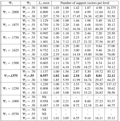
When solving the constrained minimization problem (8) (cf. Appendix A), we find the optimal numbers n∗₁, ...,n∗₆of support vectors, rounded to the nearest even integer, are given by:

n∗={2, 2,2, 4,8,22},

(cf. table 2), corresponding toΨ∗= ((Ψ−₁1)∗,Ψ∗₂) = (7.27,0.55), resulting in β∗_{={7.27,25.21,87.39, 302.95,525.09,910.11}. For example, we estimate}

P0(groot >0) =

1

2×7.27 =0.069

the false positive rate at the root.

The empirical conditional false alarms were estimated on background patterns taken from 200 images including highly textured areas (flowers, houses, trees, etc.). The conditional false positive rates for the model and the empirical results are quite similar, so that the cost in the objective function (8) approximates effectively the observed cost. In fact, when evaluating the objective

function in (8), the average cost was 3.379 kernel evaluations per pattern whereas in practice this

average cost was 3.196 per pattern taken from scenes including highly textured areas.

Again, the coefficientsβ∗_l and the complexity n∗_l of the SVM classifiers are increasing as we go down the hierarchy, which demonstrates that the best architecture of the g-network is low-to-high in complexity.

7.4 Features and Parameters

Many factors intervene in fitting our cost/error model to real observations (the conditional false alarms), including the size of the training sets and the choice of features, kernels and other parame-ters, such as the bound on the expected number of false alarms. Obviously the nature of the resulting g-network can be sensitive to variations of these factors. We have only used wavelet features, the Gaussian kernel, selecting the parameters by cross-validation, and the very small ORL database.

Ψ1 Ψ2 L1error Number of support vectors per level

Ψ2=.70 0.980 1.03 1.08 1.42 1.87 4.98 16.375

Ψ1=.2000 Ψ2=.55 0.809 1.49 2.35 3.69 4.99 11.64 32.12

Ψ2=.30 1.207 2.70 8.13 17.45 24.36 42.89 93.50

Ψ2=.70 1.129 1.00 1.08 1.46 1.98 5.40 18.12

Ψ1=.1875 Ψ2=.55 0.750 1.39 2.20 3.46 4.68 10.91 30.12

Ψ2=.30 1.367 2.53 7.62 16.36 22.83 40.20 87.62

Ψ2=.70 0.995 1.00 1.18 1.70 2.46 7.20 25.50

Ψ1=.1750 Ψ2=.55 0.766 1.30 2.05 3.23 4.37 10.19 28.12

Ψ2=.30 1.401 2.36 7.12 15.27 21.32 37.56 81.87

Ψ2=.70 0.981 1.00 1.29 2.00 3.13 9.84 37.00

Ψ1=.1625 Ψ2=.55 0.752 1.21 1.91 3.00 4.06 9.46 26.12

Ψ2=.30 1.428 2.19 6.61 14.18 19.80 34.86 76.00

Ψ2=.70 0.839 1.00 1.41 2.38 4.03 13.74 55.12

Ψ1=.1500 Ψ2=.55 0.605 1.11 1.76 2.77 3.75 8.74 24.12

Ψ2=.30 1.339 2.02 6.10 13.09 18.27 32.17 70.12

Ψ2=.70 1.137 1.00 1.56 2.87 5.30 19.72 85.12

Ψ1=.1375 Ψ2=.55 0.557 1.02 1.61 2.54 3.43 8.01 22.12

Ψ2=.30 1.580 1.85 5.59 11.99 16.74 29.47 64.25

Ψ2=.70 1.230 1.00 1.75 3.53 7.16 29.29 137.12

Ψ1=.1250 Ψ2=.55 0.808 1.00 1.71 2.89 4.21 10.56 30.62

Ψ2=.30 1.441 1.69 5.08 10.91 15.23 26.83 58.50

Ψ2=.70 NS - - -

-Ψ1=.1000 Ψ2=.55 0.958 1.00 2.21 4.69 8.60 27.23 93.37

Ψ2=.30 0.687 1.35 4.06 8.72 12.18 21.44 46.75

Ψ2=.70 NS - - -

-Ψ1=.0750 Ψ2=.55 NS - - -

-Ψ2=.30 1.242 1.01 3.05 6.55 9.14 16.11 35.12

Table 2: A sample of the simulation results. Shown, for selected values of (Ψ1, Ψ2), are the L1

error in (10) and also the numbers of support vectors which minimize cost. In practice 10×10 possible values ofΨ1andΨ2 are considered (Ψ1∈[0,0.2]andΨ2∈[0.1,1.0]).

(NS stands for “no solution”, L1refers to the sum of absolute differences, and the bold line

is the optimal solution.)

were abandoned due to extensive computation; their performance is unknown. Similar arguments apply to the choice of kernels and their parameters; for instance the scale of the Gaussian kernel controls influences both the error rate and the number of support vectors in the f-network (and also in the g-network.)

8. Experiments

All the training images of faces are based on the Olivetti database of 400 gray level pictures – ten frontal images for each of forty individuals. The coordinates of the eyes and the mouth of each picture were labeled manually. Most other methods (see below) use a far larger training set, in fact, usually ten to one hundred times larger. In our view, the smaller the better in the sense that the number of examples is a measure of performance along with speed and accuracy. Nonetheless, this criterion is rarely taken into account in the literature on face detection (and more generally in machine learning).

In order to sample the pose variation within Λt, for each face image in the original Olivetti

database, we synthesize 20 images of 64×64 pixels with randomly chosen poses in Λt. Thus, a

set of 8,000 faces is synthesized for each pose cell in the hierarchy. Background information is

collected from a set of 1,000 images taken from 28 different topical databases (including

auto-racing, beaches, guitars, paintings, shirts, telephones, computers, animals, flowers, houses, tennis,

trees and watches), from which 50,000 subimages of 64×64 pixels are randomly extracted.

Given coarse-to-fine search, the “right” alternative hypothesis at a node is “path-dependent”. That is, the appropriate “negative” examples to train against at a given node are those data points which pass all the tests from the root to the parent of the node. As with cascades, this is what we do in practice; more precisely, we merge a fixed collection of background images with a “path-dependent” set (for details see Sahbi, 2003, chap. 4).

Each subimage, either a face or background, is encoded using the 16×16 low frequency

coef-ficients of the Haar wavelet transform computed efficiently using the integral image (Sahbi, 2003; Viola and Jones, 2001). Thus, only the coefficients of the third layer of the wavelet transform are

used; see Chapter 2 of Sahbi (2003). The set of face and background patterns belonging toΛt are

used to train the underlying SVM ft in the f-network (using a Gaussian kernel).

8.1 Clustering Detections

Generally, a face will be detected at several poses; similarly, false positives will often be found in small clusters. In fact, every method faces the problem of clustering detections in order to provide a reasonable estimate of the “false alarm rate,” rendering comparisons somewhat difficult.

The search protocol was described in Section 7.1. It results in a set of detections Dg for each

non-overlapping 16×16 block in the original image and each such block in each of three

downsam-pled images (to detect larger faces). All these detections are initially collected. Evidently, there are many instances of two “nearby” poses which cannot belong to two distinct, fully visible faces. Many ad hoc methods have been designed to ameliorate this problem. We use one such method adapted to our situation: For each hierarchy, we sum the responses of the SVMs at the leaves of each complete chain (i.e., each detection in Dg) and remove all the detections from the aggregated list unless this

sum exceeds a learned thresholdτ, in which case Dgis represented by a single “average” pose. In

not increase due to pruning and yet some false positives are removed. Incompatible detections can and do remain.

Note: One can also implement a “voting” procedure to arbitrate among such remaining but

incom-patible detections. This will further reduce the false positive rate but at the expense of some missed detections. We shall not report those results; additional details can be found in Sahbi (2003). Our main intention is to illustrate the performance of the g-network on a real pattern recognition problem rather than to provide a detailed study of face detection or to optimize our error rates.

8.2 Evaluation

We evaluated the g-network in term of precision and run-time in several large scale experiments involving still images, video frames (TF1) and standard datasets of varying difficulty, including the CMU+MIT image set; some of these are extremely challenging. All our experiments were run under a 1-Ghz pentium-III mono-processor containing a 256 MB SDRM memory, which is today a standard machine in digital image processing.

The Receiver Operator Characteristic (ROC) curve is a standard evaluation mechanism in ma-chine perception, generated by varying some free parameter (e.g., a threshold) in order to investigate the trade-off between false positives and false negatives. In our case, this parameter is the threshold

τfor the aggregate SVM score of complete chains discussed in previous section. Several points on

the ROC curve are given for the TF1 and CMU+MIT test sets whereas only a single point is reported for easy databases (such as FERET).

8.2.1 FERETANDTF1 DATASETS

The FERET database (FA and FB combined) contains 3,280 images of single and frontal views of

faces. It is not very difficult: The detection rate is 98.8 % with 245 false alarms and examples are

shown in the top of Fig 10. The average run time on this set using a 1Ghz is 0.28 (s) for images of

size 256×384.

The TF1 corpus involves a News-video stream of 50 minutes broadcasted by the French TV channel TF1 on May 5th, 2002. (It was used for a video segmentation and annotation project at

INRIA and is not publicly available.) We sample the video at one frame each 4(s), resulting into

750 good quality images containing 1077 faces. Some results are shown on the bottom of Fig 10 and the performance is described in Table 8.2.1 for three points on the ROC curve. The false alarm

rate is the total number of false detections divided by the total number of hierarchies traversed, that

is, the total number of 16×16 blocks visited in processing the entire database.

8.2.2 ARF DATABASE ANDSENSITIVITYANALYSIS

The full ARF database contains 4000 images on ten DVDs; eight of these DVDs – 3,200 images

with faces of 100 individuals against uniform backgrounds – are publicly available at

(http://rvl1.ecn.purdue.edu/∼aleix/aleix face DB.html). This dataset is still very challenging due

Figure 10: Sample detections on three databases: FERET (top), ARF (middle), TF1 (bottom).

are due to occlusion of the mouth, 56 % due to occlusion of the eyes (presence of sun glasses) and 11.88 % due to face shape variation and lighting effects.

8.2.3 CMU+MIT DATASET

The CMU subset contains frontal (upright and in-plane rotated) faces whereas the MIT subset

con-tains lower quality face images. Images with an in-plane rotation of more than 200were removed,