Comments on the “Core Vector Machines: Fast SVM Training on Very
Large Data Sets”
Gaëlle Loosli [email protected]
Stéphane Canu [email protected]
LITIS, INSA de Rouen Avenue de l’Université
76801 Saint-Etienne du Rouvray France
Editor: Nello Cristianini
Abstract
In a recently published paper in JMLR, Tsang et al. (2005) present an algorithm for SVM called Core Vector Machines (CVM) and illustrate its performances through comparisons with other SVM solvers. After reading the CVM paper we were surprised by some of the reported results. In order to clarify the matter, we decided to reproduce some of the experiments. It turns out that to some extent, our results contradict those reported. Reasons of these different behaviors are given through the analysis of the stopping criterion.
Keywords: SVM, CVM, large scale, KKT gap, stopping condition, stopping criteria
1. Introduction
In a recently published paper in JMLR, Tsang et al. (2005) present an algorithm for SVM, called CVM. In this paper, some illustration of the CVM performances, compared to others solvers are shown. We have been interested in reproducing their results concerning the checkers problem be-cause we knew that SimpleSVM (Vishwanathan et al., 2003) could handle such a problem more efficiently than reported in the paper. Tsang et al. (2005, Figure 3, page 379) show that CVM’s training time is independent of the sample size and obtains similar accuracies to the other SVM solvers. We discuss those results through the analysis of the stopping criteria of the different solvers and the effects of hyper-parameters.
Coming back to the comparison of solvers, our first experiment (Section 2) shows how different sets of hyper-parameters produce different behaviors for both CVM and SimpleSVM. We also give results with libSVM (Chang and Lin, 2001a) for the sake of comparison since SMO (Platt, 1999) is a standard in SVM resolution. Our results indicates that the choice of the hyper-parameters for CVM does not only influence the training time but also greatly the performance (more than for the other methods).
Section 3 aims at understanding what influences the most the CVM accuracy. We show that CVM uses a stopping criterion which may induce complex tuning and unexpected results. We also explore the behavior of CVM when C varies compared to libSVM and SimpleSVM.
In Section 4, our second experiment points out that the choice of the magnitude of the hyper-parameter C (which behaves as a regulator) is critical, more than the bandwidth for this problem. It is interesting to notice that each method has modes that are favorable and modes that are not. The last experiments enlightens those different modes.
103 104 105 106
104 c p u t ra in in g t im e ( lo g )
103 104 105 106
101 102 103 104 105
Training size (log)
N u m b e r o f s u p p o rt v e c to rs ( lo g )
103 104 105 106
0 5 10 15 20
Training size (log)
E rr o r ra te ( % )
103 104 105 106
100 104
Training size (log)
c p u t ra in in g t im e ( lo g )
103 104 105 106
0 5 10 15 20
Training size (log)
E rr o r ra te ( % )
103 104 105 106
105
Training size (log)
N u m b e r o f s u p p o rt v e c to rs ( lo g
) 4 5 6
100 104
Training size (log)
c p u t ra in in g t im e ( lo g )
103 104 105 106
0 5 10 15 20
Training size (log)
E rr o r ra te ( % )
103 104 105 106
101 102 103 104 105
Training size (log)
N u m b e r o f s u p p o rt v e c to rs ( lo g )
103 104 105 106
0 5 10 15 20
Training size (log)
E rr o r ra te ( % )
103 104 105 106
105 104
103
102
101
Training size (log)
N u m b e r o f s u p p o rt v e c to rs ( lo g )
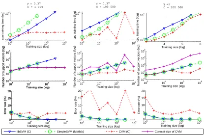
libSVM (C) SimpleSVM (Matlab) CVM (C) Coreset size of CVM
γ = 0.37
C = 1 000
γ = 0.37
C = 100 000 γ
=1 C = 100 000
About the Reproducibility All experiments presented here can be reproduced with codes and data set that are all published.
• CVM (Tsang et al., 2005) Version 1.1 (in C) downloaded fromhttp://www.cs.ust.hk/
~ivor/cvm.htmlfor Linux platform on the 3rd of April 2006.
• LibSVM (Chang and Lin, 2001a) We used the release contained in CVM (here we should
mention that a new version of libSVM exists (Fan et al., 2005), which would probably give some better results).
• SimpleSVM (Vishwanathan et al., 2003; Loosli, 2004) We used version 2.3 available at
http://asi.insa-rouen.fr/~gloosli/coreVSsimple.html, written in Matlab.
• Data We have published the used data sets at http://asi.insa-rouen.fr/~gloosli/
coreVSsimple.html, in both formats for libSVM and SimpleSVM.
Note that all results presented here are obtained using a stopping toleranceε=10−6 as proposed in the CVM paper. Moreover, from now and for the rest of the paper, SimpleSVM will refer to the specific version implemented in the toolbox, as well as SMO will refer to the libSVM implementa-tion.
2. Alternative Parameters For the Checkers
This section aims at verifying that SimpleSVM can treat one million points in problems like the checkers with adapted hyparameters. On the way, we also see that this leads to better per-formance than the one presented on Figure 3 page 379 of Tsang et al. (2005) and not only for SimpleSVM.
2.1 Original Settings
We used the parameters described in their paper (γ=0.37 and C=1000), γbeing fixed to this value so the results can easily be reproduced (the setting of the paper relies on the average distance of couples of points on the training set). Note thatγ=1/βcorresponds to the hyper-parameters directly given to the toolboxes - k(xi,xj) =exp −γ(xi−xj)2
and thatβis the notation used in the studied paper. Results are presented on Figure 1, first column.
2.2 Others Settings
Our motivation is that the checkers is a separable problem. First, this should reduce the number of support vectors and second, it should be possible to have a zero error in test. Thus we used in a second time some other hyper-parameters : the coupleγ=0.37, C=100000 on the one hand and
γ=1 and C =100000 on the second hand (found by cross-validation). Examples of results are presented on Figure 1, second and third columns.1
2.3 Results
• For the given settings, we can see similar behaviors as the one presented in the paper concern-ing trainconcern-ing size, performance and speed. In particular, due to the large number of support vectors required for this setting (graph (b), Figure 1), SimpleSVM cannot be run over 30,000 data points,
• the possibility to run SimpleSVM or CVM until 1 million points depends on the settings,
• both SimpleSVM and libSVM achieve a 0 testing error (which means to us that the settings are more adapted) while CVM shows a really unstable behavior regarding testing error,
• for CVM, training time grows very fast for large values of C, due to huge intermediate number of active points (see Section 4), even if it still gives a sparse solution in the end,
• finally, the training error shows that CVM does not converge towards the solution for all hyper-parameters.
3. Study of CVM
Because Figure 1 shows very different behaviors of the algorithms, we focus in this part on the stopping criteria and on the role played by the different hyper-parameters. To do so we first compare CVM and SimpleSVM algorithms and then we point out that stopping criteria are different and may explain the results reported in Figure 1. We illustrate our claims on Figure 2 which shows that the magnitude of C is the key hyper-parameter to explore the different behaviors of the algorithms.
3.1 Algorithm
The algorithm presented in CVM uses MEB (Minimum Enclosing Balls) but can also be closely related to decomposition methods (such as SimpleSVM). Both methods consist in two alternating steps, one that defines groups of points and the other that computes theα(the Lagrangian multipliers involved in the dual of the SVM, see Schölkopf and Smola, 2002). In order to make clear that CVM and SimpleSVM are similar, we briefly explain those steps for each. Doing so we also enlighten their differences. Then we give the two algorithms and specify where stopping conditions apply.
3.1.1 DEFINING THEGROUPS
CVM: divides the database between useless and useful points. The useful points are designated as the coreset and correspond to all the points that are candidates to be support vectors. This set can only grow since no removing step is done. Among the points of the coreset, not all are support vectors in the end.
SimpleSVM: divides the database into three groups: Iw for the non bounded support vectors
(0<αw<C), IC for the bounded points - misclassified or in the margins (αC=C) and I0 which
contains the non support vectors (α0=0).
3.1.2 FINDING THEα
SimpleSVM: solves an optimization problem such that the optimality condition leads to a linear system. This linear system hasαwas unknown.
3.1.3 ALGORITHMS
CVM: uses the following steps:
Algorithme 1 CVM algorithm
1: initialize .two points in the coreset, the first center of the ball, the first radius (see the original paper for details on the MEB)
2: if no point in the remaining points falls outside theε-ball then
3: stop (withε-tolerance) .outer loop
4: end if
5: take the furthest point from the center of the current ball, add it to the core set
6: solve the QP problem on the points contained in the coreset (using SMO with warm start with
ε-tolerance) .inner loop
7: update the ball (center and radius)
8: go to second step
Two things require computational efforts there: the distance computation involved in steps 2 and 5, and solving the QP in step 6. For the distance computation, the authors propose a heuristics that consists of sampling 59 points instead of checking all the points, thus reducing greatly the time required. Doing so they ensure at 95% that the furthest point among those 59 points is part of the 5% of points the furthest from the center. For step 6, they use warm start feature of the SMO algorithm, doing a rank-one update of the QP.
SimpleSVM: uses the following steps:
Algorithme 2 SimpleSVM algorithm
1: initialize .two points in Iw, first values ofαw
2: if no point in the remaining points is misclassified by the current solution then
3: stop (withε-tolerance)
4: end if
5: take the furthest misclassified point from the frontier, add it to Iw
6: update the linear system and retrieveαw
7: if all 0<αw<C then
8: go to second step
9: else
10: remove violating point from Iw(put it in I0or Icdepending on the constraint it violates) and go to step 6
11: end if
3.2 Stopping Criteria
We now consider the stopping criteria used in those algorithms. Indeed we have noted in the previ-ous algorithms steps where a stopping criteria is involved (theε-tolerance).
For the sake of clarity, we will also give details about theν-SVM. Indeed, we will see that the CVM stopping criterion is analog to theν-SVM one.
Notations and definitions Let x be our data labeled with y. Let k(., .)be the kernel function. We
will denoteαthe vector of Lagrangian multipliers involved in the dual problem of SVMs.
K is the kernel, such that Ki j=yiyjk(xi,xj). As defined in Tsang et al. (2005, Eq. 17), ˜K is the
modified kernel, such that ˜Ki j=yiyjk(xi,xj) +yiyj+δCi j (δi j=1 if i=j and 0 otherwise). ˜K is used for the reformulation of the SVM as a MEB problem.
As defined in Tsang et al. (2005, page 370), ˜K=Kii˜ =K+1+1
C withK=Kii(which is equal to 1 for the RBF kernel).
1 stands for vectors of ones, 0 for vectors of zeros. All vectors are columns unless followed by
a prime.
C-SVM type (SimpleSVM and SMO) The stopping criterion commonly used in classical SVM
(C-SVM) is
min(Kα1−1)≥ −ε1.
The two implementations SimpleSVM and libSVM (the C-SVM version) use similar stopping cri-teria, up to the biased term. This corresponds to the constraint of good classification. Here the magnitude of α, influenced by C, slightly modifies the tightness of the stopping condition. For SMO, a very strict stopping criteria causes a large number of iterations and slows down the training speed. This is the reason why it is usually admitted that SMO should not be run with large C values (and this idea is often extended to SVM independently of the solver, which is a wrong shortcut). On the other hand, SimpleSVM’s training speed is linked to the number of support vectors (there is no direction search with a first order gradient to slow it down). For separable problems, large C produces sparser solutions, so SimpleSVM is faster with large C.
ν-SVM type In theν-SVM setting (see Chen et al., 2005, for further details), the stopping criterion
is
min(Kα2−ρ21)≥ −ε2
whereρ2corresponds to the margin (see Chang and Lin, 2001b, for derivations). In order to compare this criterion to the previous one, it is possible to exhibit links between the two problems. Let say that for a given problem and a givenε2, theν-SVM optimal solution isα2 andρ2. To obtain the same solution using the C-SVM, one can use the following relations: C=1/ρ2(see Schölkopf and Smola, 2002, p209, prop. 7.6) andε1=ε2/ρ2. The solutionα1obtained by the C-SVM can also be compared toα2since we know that 0≤α2≤1 and 0≤α1≤C. Thus there isα2=α1/C. Thanks to those relations it is possible to express the C-SVM stopping criterion with theν-SVM terms by setting
ε1=ε2C= ε2 ρ2.
CVM CVM uses two overlapping loops. The outer one for the coreset selection and the inner one to solve the QP problem on the coreset. Thus CVM require two stopping criteria, one per loop.
Let us first consider the inner loop, that is, points that are constituting the coreset. The related multipliersα3are found using SMO. However, as mentioned in Tsang et al. (2005, Equation 5), the solved QP is similar to aν-SVM problem. Hence the stopping condition is similar to theν-SVM stopping condition. The major difference between aν-SVM and the inner loop of CVM is the use of a modified kernel ˜K instead of K. The leading stopping criterion is the one of the outer loop.
The stopping criterion of the outer loop (equivalent to Eq. 25 of the paper) is:
min (K˜α3)R −ρ31≥ −ε3K˜
where
R
indicates points that are outside the coreset. Note that if α3 is the CVM solution for a given ε3, since 10α3=1, the equivalent solution α1 given by a C-SVM is linked as follows :α3=α1/(10α1). Moreover, settingρ3=1/(10α1), using those relations and expanding the kernel expression give:
min (K+yy 0+1
CId)α1
R −1
10α1
≥ −ε3(K+1+1
C). (1)
Here again thanks to those relations it is possible to express the C-SVM stopping criterion with the outer CVM terms by taking
ε1= ε3(K+1+ 1
C) + (yy
0+1
CId)α3
`
ρ3
where`denotes the indice of the point minimizing the left-hand side part of (1). We can observe a similar scale effect to the one happening forν-SVM.
Apart from the possibility to compare fairly to other solvers, let us study the behavior of CVM depending on C or on the training set size.
• The modified kernel hides a non-negligible regularizing effect. Indeed 1/C is added to the diagonal. Thus for small C, the kernel becomes well conditioned. Hence we can expect CVM to give better results with small C.
• From its ν-SVM like form, it also gets stricter condition for small C. This strict condition increases the number of steps and, as a side effect, the probability to check more points outside the coreset when sampling the 59 points.
Overall, for a small C, CVM should be slower than SMO (since it repeats SMO) and give accurate results.
• A large C, on the contrary, does not influence the kernel conditioning anymore.
• From the form of the stopping criterion, the condition is looser.
• The inner stopping condition is loose too. The looser it is, the fewer support vectors it takes.
Overall, we can expect less accurate results for large C.
4. Experimental Results
We now propose experiments illustrating the previous analysis. We first make the training size varies and then C. For all the experiments, we useε=10−6.
Behavior of the algorithms when size is growing Figure 2 shows the results for experiments
where the training size is growing for various sets of hyper-parameters. We observe:
• for a given C, results are similar in terms of training time, regardless of the kernel bandwidth,
• the best configuration for CVM is medium C regarding training time and small C regarding accuracy,
• for small C, CVM is the most accurate method (due to a regularization on the kernel),
• for large C, CVM accuracy tends to decrease.
It is clear from this experiment that we face different behaviors depending on the hyper-parameters. Each method has a favorable mode and those are not compatible. Since the bandwidth does not influence the trends of the obtained curves, we will fix it and focus now on variations of C.
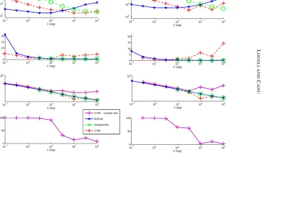
Behavior of the algorithms when C is varying Figure 3 shows how the training changes
de-pending on the value of C for each studied algorithm. The same experiment is conducted for two training sizes (10,000 points for the first column, 30,000 for the second), in order to point out that the training size amplifies sensitivity of CVM to its hyper-parameters. Each experiment reports the training time (top figure), the error rate (second figure), the number of support vectors and the size of the coreset (third figure) and the proportion of support vectors in the coreset for CVM (last figure), C∈[10−2,106].
small C SimpleSVM fails because of not enough memory, libSVM is the fastest (loose stopping
condition) and CVM the most accurate (regularized kernel). The coreset size corresponds almost exactly to the number of support vectors, which means that the selection criterion is accurate.
large C SimpleSVM is faster than libSVM (penalized by strict stopping condition) and both are as
accurate. CVM gets large error rate and we see that the less the coreset set is related to the support vectors, the less accurate the method is. The point that is not so clear is the reason why the coreset grows that much and this is still to be explored.
5. Conclusion
In their conclusion, the authors claim that “experimentally, it [CVM] is as accurate as existing SVM implementations”. We show that is not always true and furthermore that it may not converge towards the solution.
Moreover we have shown that comparisons between CVM and usual SVM solvers should be careful since the stopping criteria are different. We have illustrated this point as well as the effect of magnitude of C on the training time. We have explained partly the behavior of CVM and shown that their results may be misleading, yet it still requires further exploration (particularly regarding the actual effects of the random sub-sampling).
C O M M E N T S O N C V M
103 104
10−1 100
101 102
103
Training size (log)
103 104
101
102 103
104
Training size (log)
103 104
0 5 10 15 20 25 30 35 40
Training size (log)
103 104
10−1 100
101 102
103
Training size (log)
103 104
101
102 103
104
Training size (log)
103 104
0 5 10 15 20 25 30 35 40
Training size (log)
103 104
10−1 100
101 102
103
Training size (log)
103 104
101
102 103
104
Training size (log)
103 104
0 5 10 15 20 25 30 35 40
Training size (log)
103 104
10−1 100
101 102
103
Training size (log)
103 104
101
102 103
104
Training size (log)
103 104
0 5 10 15 20 25 30 35 40
Training size (log)
103 104
10−1 100
101 102
103
Training size (log)
103 104
101
102 103
104
Training size (log)
103 104
0 5 10 15 20 25 30 35 40
Training size (log)
103 104
10−1 100
101 102
103
Training size (log)
103 104
101
102 103
104
Training size (log)
103 104
0 5 10 15 20 25 30 35 40
Training size (log) CVM
LibSVM SimpleSVM
Results for C = 1 Left : γ = 1 Right γ = 0.3
Results for C = 1000 Left : γ = 1 Right γ = 0.3
Results for C = 1000000 Left : γ = 1 Right γ = 0.3
L O O S L I A N D C A N U
10−2 100 102 104 106
100 102 104
C (log)
10−2 100 102 104 106
0 5 10 15 20 C (log)
10−2 100 102 104 106
105
C (log)
10−2 100 102 104 106
0 50 100
C (log)
10−2 100 102 104 106
100 102 104
C (log)
10−2 100 102 104 106
0 5 10 15 20 C (log)
10−2 100 102 104 106
105
C (log)
10−2 100 102 104 106
0 50 100
C (log) CVM − coreset size
libSVM SimpleSVM CVM Training time (cpu seconds) in log scale Error rate on 2000 unseen points Number of support vectors (and size of the coreset for CVM) For CVM, proportion of points from the coreset selected as support vectors
Results obtained on 10000 training points Results obtained on 30000 training points
here an adaptiveεin order to avoid unstable behaviors but it can not be done easily. Furthermore, one who uses SVM should be aware that each method has favorable and non favorable ranges of hyper-parameters.
Finally, we acknowledge that a fast heuristic which achieves loose yet still acceptable accuracy is interesting and useful for very large databases (by itself or as a starting point for more accurate methods) but to use it with confidence, one has to know when the method is indeed accurate enough. Hence CVM may benefit from being presented along with its limits.
Acknowledgments
We would like to thank very much the anonymous reviewers for helpful comments on the stopping conditions. This work was supported in part by the IST Programme of the European Community, under the PASCAL Network of Excellence, IST-2002-506778. This publication only reflects the authors’ views.
References
Chih-Chung Chang and Chih-Jen Lin. LIBSVM: a library for support vector machines, 2001a. URL
http://www.csie.ntu.edu.tw/~cjlin/libsvm.
Chih-Chung Chang and Chih-Jen Lin. Trainingν-support vector classifiers: Theory and algorithms. Neural Computation, (9):2119–2147, 2001b.
Pai-Hsuen Chen, Chih-Jen Lin, and Bernhard Schölkopf. A tutorial on v-support vector machines. Applied Stochastic Models in Business and Industry, 21(2):111–136, 2005.
Rong-En Fan, Pai-Hsuen Chen, and Chih-Jen Lin. Working set selection using second order infor-mation for training support vector machines. Journal of Machine Learning Research, 2005.
Gaëlle Loosli. Fast svm toolbox in Matlab based on SimpleSVM algorithm, 2004. http://asi. insa-rouen.fr/~gloosli/simpleSVM.html.
John Platt. Fast training of support vector machines using sequential minimal optimization. In B. Scholkopf, C. Burges, and A. Smola, editors, Advanced in Kernel Methods - Support Vector Learning, pages 185–208. MIT Press, 1999.
Bernhard Schölkopf and Alexander J. Smola. Learning with Kernels. MIT Press, 2002.
Ivor W. Tsang, James T. Kwok, and Pak-Ming Cheung. Core vector machines: Fast SVM training on very large data sets. J. Mach. Learn. Res., 6:363–392, 2005.