Estimating the “Wrong” Graphical Model: Benefits in the
Computation-Limited Setting
Martin J. Wainwright [email protected]
Department of Statistics
Department of Electrical Engineering and Computer Sciences University of California at Berkeley
Berkeley, CA 94720, USA
Editor: Max Chickering
Abstract
Consider the problem of joint parameter estimation and prediction in a Markov random field: that is, the model parameters are estimated on the basis of an initial set of data, and then the fitted model is used to perform prediction (e.g., smoothing, denoising, interpolation) on a new noisy observa-tion. Working under the restriction of limited computation, we analyze a joint method in which the same convex variational relaxation is used to construct an M-estimator for fitting parameters, and to perform approximate marginalization for the prediction step. The key result of this paper is that in the computation-limited setting, using an inconsistent parameter estimator (i.e., an estimator that returns the “wrong” model even in the infinite data limit) is provably beneficial, since the resulting errors can partially compensate for errors made by using an approximate prediction technique. En route to this result, we analyze the asymptotic properties of M-estimators based on convex varia-tional relaxations, and establish a Lipschitz stability property that holds for a broad class of convex variational methods. This stability result provides additional incentive, apart from the obvious benefit of unique global optima, for using message-passing methods based on convex variational relaxations. We show that joint estimation/prediction based on the reweighted sum-product algo-rithm substantially outperforms a commonly used heuristic based on ordinary sum-product.
Keywords: graphical model, Markov random field, belief propagation, variational method, pa-rameter estimation, prediction error, algorithmic stability
1. Introduction
Graphical models such as Markov random fields (MRFs) are widely used in many application do-mains, including machine learning, natural language processing, statistical signal processing, and communication theory. A fundamental limitation to their practical use is the difficulty associated with computing various statistical quantities (e.g., marginals, data likelihoods etc.); such quantities are of interest both Bayesian and frequentist settings. Sampling-based methods, especially those of the Markov chain Monte Carlo (MCMC) variety (Liu, 2001; Robert and Casella, 1999), repre-sent one approach to obtaining stochastic approximations to marginals and likelihoods. A possible disadvantage of sampling methods is their relatively high computational cost. It is thus of consider-able interest for various application domains to consider less computationally intensive methods for generating approximations to marginals, log likelihoods, and other relevant statistical quantities.
marginal probabilities can be reformulated as a convex optimization problem; see Yedidia (2001) or Wainwright and Jordan (2003) for overviews. Although this optimization problem is intractable to solve exactly for general MRFs, it suggests a principled route to obtaining approximations— namely, by relaxing the original optimization problem, and taking the optimal solutions to the re-laxed problem as approximations to the exact values. In many cases, optimization of the rere-laxed problem can be carried out by “message-passing” algorithms, in which neighboring nodes in the Markov random field convey statistical information (e.g., likelihoods) by passing functions or vec-tors (referred to as messages). Well-known examples of such variational methods include mean field algorithms, the belief propagation or sum-product algorithm, as well as various extensions including generalized belief propagation and expectation propagation.
Estimating the parameters of a Markov random field from data poses another significant chal-lenge. A direct approach—for instance, via (regularized) maximum likelihood estimation—entails evaluating the cumulant generating (or log partition) function, which is computationally intractable for general Markov random fields. One viable option is the pseudolikelihood method (Besag, 1975, 1977), which can be shown to produce consistent parameter estimates under suitable assumptions, though with an associated loss of statistical efficiency. Other researchers have studied algorithms for ML estimation based on stochastic approximation (Younes, 1988; Benveniste et al., 1990), which again are consistent under appropriate assumptions, but can be slow to converge.
1.1 Overview
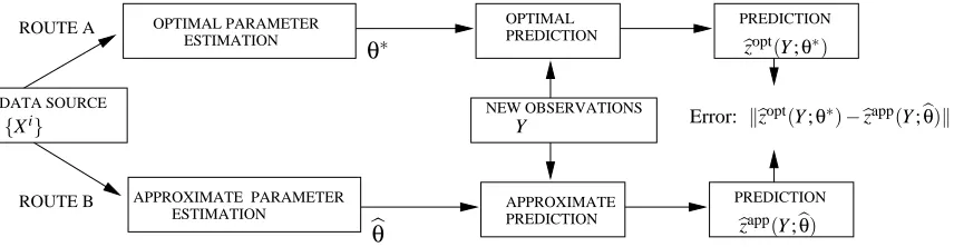
As illustrated in Figure 1, the problem domain of interest in this paper is that of joint estimation and prediction in a Markov random field. More precisely, given samples{X1, . . . ,Xn}from some un-known underlying model p(·;θ∗), the first step is to form an estimate of the model parameters. Now suppose that we are given a noisy observation of a new sample path Z∼p(·;θ∗), and that we wish to form a (near)-optimal estimate of Z using the fitted model, and the noisy observation (denoted Y ). Examples of such prediction problems include signal denoising, interpolation of missing data, and sentence parsing. Disregarding any issues of computational cost and speed, one could proceed via Route A in Figure 1—that is, one could envisage first using a standard technique (e.g., regularized maximum likelihood) for parameter estimation, and then carrying out the prediction step (which might, for instance, involve computing certain marginal probabilities) by Monte Carlo methods.
This paper, in contrast, is concerned with the computation-limited setting, in which both sam-pling or brute force methods are overly intensive. With this motivation, a number of researchers have studied the use of approximate message-passing techniques, both for problems of predic-tion (Heskes et al., 2003; Ihler et al., 2005; Minka, 2001; Mooij and Kappen, 2005b; Tatikonda, 2003; Wainwright et al., 2003a; Wiegerinck, 2005; Yedidia et al., 2005) as well as for parameter estimation (Leisink and Kappen, 2000; Sutton and McCallum, 2005; Teh and Welling, 2003; Wain-wright et al., 2003b). However, despite their wide-spread use, the theoretical understanding of such message-passing techniques remains limited1, especially for parameter estimation. Consequently, it is of considerable interest to characterize and quantify the loss in performance incurred by using computationally tractable methods versus exact methods (i.e., Route B versus A in Figure 1). More
specifically, our analysis applies to variational methods that are based on convex relaxations. This class includes a number of existing methods—among them the tree-reweighted sum-product algo-rithm (Wainwright et al., 2005), reweighted forms of generalized belief propagation (Wiegerinck, 2005), and semidefinite relaxations (Wainwright and Jordan, 2005). Moreover, it is possible to modify other variational methods—for instance, expectation propagation (Minka, 2001)—so as to “convexify” them.
APPROXIMATE PARAMETER ESTIMATION
ESTIMATION OPTIMAL PARAMETER
APPROXIMATE PREDICTION OPTIMAL PREDICTION
DATA SOURCE
PREDICTION PREDICTION
ROUTE A
ROUTE B
NEW OBSERVATIONS
PSfrag replacements
{Xi}
bθ
θ∗ bzopt(Y ;θ∗)
b zapp(Y ;bθ)
Y Error: kbz
opt(Y ;θ∗)−bzapp(Y ;bθ)k
Figure 1: Route A: computationally intractable combination of parameter estimation and predic-tion. Route B: computationally efficient combination of approximate parameter estima-tion and predicestima-tion.
1.2 Our Contributions
At a high level, the key idea of this paper is the following: given that approximate methods can lead to errors at both the estimation and prediction phases, it is natural to speculate that these sources of error might be arranged to partially cancel one another. The theoretical analysis of this paper confirms this intuition: we show that with respect to end-to-end performance, it is in fact beneficial, even in the infinite data limit, to learn the “wrong” the model by using inconsistent methods for parameter estimation. En route to this result, we analyze the asymptotic properties of M-estimators based on convex variational relaxations, and establish a Lipschitz stability property that holds for a broad class of variational methods. Such global algorithmic stability is a fundamental concern given statistical models imperfectly estimated from limited data, or for applications in which “er-rors” may be introduced into message-passing (e.g., due to quantization or other forms of communi-cation constraints in sensor networks). Thus, our global stability result provides further theoretical justification—apart from the obvious benefit of unique global optima—for using message-passing methods based on convex variational relaxations. Finally, we provide some empirical results to show that joint estimation/prediction based on the reweighted sum-product algorithm substantially outperforms a commonly used heuristic based on ordinary sum-product.
and prediction methods, with particular emphasis on the mixture-of-Gaussians observation model. In Section 7, we provide experimental results on the performance of a joint estimation/prediction method based on the tree-reweighted Bethe surrogate, and compare it to a heuristic method based on the ordinary belief propagation algorithm. We conclude in Section 8 with a summary and discussion of directions for future work.
2. Background
We begin with background on Markov random fields. Consider an undirected graph G= (V,E), consisting of a set of vertices V ={1, . . . ,N}and an edge set E. We associate to each vertex s∈V
a multinomial random variable Xstaking values in the set
X
s={0,1, . . . ,m−1}. We use the lowercase letter xsto denote particular realizations of the random variable Xs in the set
X
s. This papermakes use of the following exponential representation of a pairwise Markov random field over the multinomial random vector X :={Xs,s∈V}. We begin by defining, for each j=1, . . . ,m−1, the {0,1}-valued indicator function
Ij[xs] :=
(
1 if xs= j
0 otherwise (1)
These indicator functions can be used to define a potential functionθs(·):
X
s→Rviaθs(xs) := m−1
∑
j=1
θs; jIj[xs] (2)
whereθs={θs; j,j=1, . . . ,m−1}is the vector of exponential parameters associated with the
po-tential. Our exclusion of the index j=0 is deliberate, so as to ensure that the collection of indicator functionsφs(xs):={Ij[xs], j=1, . . . ,m−1}remain affinely independent. In a similar fashion, we
define for any pair(s,t)∈E the pairwise potential function
θst(xs,xt) := m−1
∑
j=1 m−1
∑
k=1
θst; jkIj[xs]Ik[xt],
where we useθst:={θst; jk, j,k=1,2, . . . ,m−1}to denote the associated collection of exponential
parameters, andφst(xs,xt):={Ij[xs]Ik[xs], j,k=1,2, . . . ,m−1}for the associated set of sufficient
statistics.
Overall, the probability mass function of the multinomial Markov random field in exponential form can be written as
p(x ;θ) = exp
∑
s∈V
θs(xs) +
∑
(s,t)∈E
θst(xs,xt)−A(θ) . (3)
Here the function
A(θ) := log h
∑
x∈XN
exp
∑
s∈V
θs(xs) +
∑
(s,t)∈E
θst(xs,xt)
i
(4)
The collection of distributions thus defined can be viewed as a regular and minimal exponential family (Brown, 1986). In particular, the exponential parameterθand the vector of sufficient statis-tics φare formed by concatenating the exponential parameters (respectively indicator functions) associated with each vertex and edge—viz.
θ = {θs,s∈V} ∪ {θst,(s,t)∈E}
φ(x) = {φs(xs),s∈V} ∪ {φst(xs,xt),(s,t)∈E}
This notation allows us to write Equation (3) more compactly as p(x ;θ) =exp{hθ,φ(x)i −A(θ)}. A quick calculation shows thatθ∈Rd, where d=N(m−1) +|E|(m−1)2is the dimension of this
exponential family.
The following properties of A are well-known:
Lemma 1 (a) The function A is convex, and strictly so when the sufficient statistics are affinely independent.
(b) It is an infinitely differentiable function, with derivatives corresponding to cumulants. In partic-ular, for any indicesα,β∈ {1, . . . ,d}, we have
∂A
∂θα =Eθ[φα(X)],
∂2A
∂θα∂θβ=covθ{φα(X),φβ(X)},
whereEθand covθ denote the expectation and covariance respectively.
We use µ∈Rd to denote the vector of mean parameters defined element-wise by µα=Eθ[φα(X)] for anyα∈ {1, . . . ,d}. A convenient property of the sufficient statisticsφdefined in Equations (1) and (2) is that these mean parameters correspond to marginal probabilities. For instance, when
α= (s; j)orα= (st; jk), we have respectively
µs; j = Eθ[Ij[xs]] =p(Xs=j ;θ), and (5a)
µst; jk = Eθ
Ij[xs]Ik[xt] =p(Xs= j,Xt =k ;θ). (5b)
3. Construction of Convex Surrogates
This section is devoted to a systematic procedure for constructing convex functions that represent approximations to the cumulant generating function. We begin with a quick development of an exact variational principle, one which is intractable to solve in general cases; see the papers (Pietra et al., 1997; Wainwright and Jordan, 2005) for further details. Nonetheless, this exact variational principle is useful, in that various natural relaxations of the optimization problem can be used to define convex surrogates to the cumulant generating function. After a high-level description of such constructions in general, we then illustrate it more concretely with the particular case of the “convexified” Bethe entropy (Wainwright et al., 2005).
3.1 Exact Variational Representation
Since A is a convex and continuous function (see Lemma 1), the theory of convex duality (Rock-afellar, 1970) guarantees that it has a variational representation, given in terms of its conjugate dual function A∗:Rd→R∪ {+∞}, of the following form
A(θ) = sup
µ∈Rd θT
In order to make effective use of this variational representation, it remains determine the form of the dual function. A useful fact is that the exponential family (3) arises naturally as the solution of an entropy maximization problem. In particular, consider the set of linear constraints
Ep[φ(X)]:=
∑
x∈XNp(x)φα(x) = µα forα=1, . . . ,d, (6)
where µ∈Rd is a set of target mean parameters. Letting
P
denote the set of all probability distri-butions with support onX
N, consider the constrained entropy maximization problem: maximize the entropy H(p):=−∑x∈XNp(x)log p(x)subject to the constraints (6).A first question is when there any distributions p that satisfy the constraints (6). Accordingly, we define the set
MARGφ(G) := µ∈Rdµ=Ep[φ(X)] for some p∈
P
,corresponding to the set of µ for which the constraint set (6) is non-empty. For any µ∈/MARGφ(G), the optimal value of the constrained maximization problem is−∞(by definition, since the problem is infeasible). Otherwise, it can be shown that the optimum is attained at a unique distribution in the exponential family, which we denote by p(·;θ(µ)). Overall, these facts allow us to specify the conjugate dual function as follows:
A∗(µ) =
(
−H(p(·;θ(µ))) if µ∈MARGφ(G)
+∞ otherwise. (7)
See the technical report (Wainwright and Jordan, 2003) for more details of this dual calculation. With this form of the dual function, we are guaranteed that the cumulant generating function A has the following variational representation:
A(θ) = max
µ∈MARGφ(G) θTµ
−A∗(µ) . (8)
However, in general, solving the variational problem (8) is intractable. This intractability should not be a surprise, since the cumulant generating function is intractable to compute for a general graphical model. The difficulty arises from two sources. First, the constraint set MARGφ(G) is extremely difficult to characterize exactly for a general graph with cycles. For the case of a multino-mial Markov random field (3), it can be seen (using the Minkowski-Weyl theorem) that MARGφ(G) is a polytope, meaning that it can be characterized by a finite number of linear constraints. The question, of course, is how rapidly this number of constraints grows with the number of nodes N in the graph. Unless certain fundamental conjectures in computational complexity turn out to be false, this growth must be non-polynomial; see Deza and Laurent (1997) for an in-depth discus-sion of the binary case. Tree-structured graphs are a notable exception, for which the junction tree theory (Lauritzen, 1996) guarantees that the growth is only linear in N.
that any Markov random field on a tree T = (V,E(T))can be factorized in terms of its marginals as follows
p(x ;θ(µ)) =
∏
s∈V
µs(xs)
∏
(s,t)∈E(T)
µst(xs,xt) µs(xs)µt(xt)
. (9)
Consequently, in this case, the negative entropy (and hence the dual function) can be computed explicitly as
−A∗(µ; T) =
∑
s∈V
Hs(µs)−
∑
(s,t)∈E(T)
Ist(µst) (10)
where Hs(µs) := −∑xsµs(xs)log µs(xs)and Ist(µst):=∑xs,xtµst(xs,xt)log
µst(xs,xt)
µs(xs)µt(xt)are the singleton entropy and mutual information, respectively, associated with the node s∈V and edge(s,t)∈E(T). For a general graph with cycles, in contrast, the dual function lacks such an explicit form, and is not easy to compute.
Given these challenges, it is natural to consider approximations to A∗ and MARGφ(G). As we discuss in the following section, the resulting relaxed optimization problem defines a convex surrogate to the cumulant generating function.
3.2 Convex Surrogates to the Cumulant Generating Function
We now describe a general procedure for constructing convex surrogates to the cumulant generating function, consisting of two main ingredients. Given the intractability of characterizing the marginal polytope MARGφ(G), it is natural to consider a relaxation. More specifically, let RELφ(G) be a convex and compact set that acts as an outer bound to MARGφ(G). We useτto denote elements of RELφ(G), and refer to them as pseudomarginals since they represent relaxed versions of local marginals. The second ingredient is designed to sidestep the intractability of the dual function: in particular, let B∗ be a strictly convex and twice continuously differentiable approximation to A∗. We require that the domain of B∗(i.e., dom(B∗):={τ∈Rd|B∗(τ)<+∞}) be contained within the relaxed constraint set RELφ(G).
By combining these two approximations, we obtain a convex surrogate B to the cumulant gen-erating function, specified via the solution of the following relaxed optimization problem
B(θ) := max
τ∈RELφ(G)
θTτ
−B∗(τ) . (11)
Note the parallel between this definition (11) and the variational representation of A in Equation (8). The function B so defined has several desirable properties, as summarized in the following proposition:
Proposition 2 Any convex surrogate B defined via (11) has the following properties:
(i) For eachθ∈Rd, the optimum defining B is attained at a unique pointτ(θ).
(ii) The function B is convex onRd.
(iii) It is differentiable onRd, and more specifically:
Proof (i) By construction, the constraint set RELφ(G)is compact and convex, and the function B∗ is strictly convex, so that the optimum is attained at a unique pointτ(θ).
(ii) Observe that B is defined by the maximum of a collection of functions linear inθ, which ensures that it is convex (Bertsekas, 1995).
(iii) Finally, the function θTτ−B∗(τ) satisfies the hypotheses of Danskin’s theorem (Bertsekas, 1995), from which we conclude that B is differentiable with∇B(θ) =τ(θ)as claimed.
Given the interpretation ofτ(θ)as a pseudomarginal, this last property of B is analogous to the well-known cumulant generating property of A—namely,∇A(θ) =µ(θ)—as specified in Lemma 1.
3.3 Convexified Bethe Surrogate
The following example provides a more concrete illustration of this constructive procedure, using a tree-based approximation to the marginal polytope, and a convexifed Bethe entropy approxima-tion (Wainwright et al., 2005). As with the ordinary Bethe approximaapproxima-tion (Yedidia et al., 2005), the cost function and constraint set underlying this approximation are exact for any tree-structured Markov random field.
Relaxed polytope: We begin by describing a relaxed version RELφ(G)of the marginal polytope MARGφ(φ). Letτsandτstrepresent a collection of singleton and pairwise pseudomarginals,
respec-tively, associated with vertices and edges of a graph G. These quantities, as locally valid marginal distributions, must satisfy the following set of local consistency conditions:
LOCALφ(G) := τ∈Rd+
∑
xs
τs(xs) =1,
∑
xtτst(xs,xt) =τs(xs) .
By construction, we are guaranteed the inclusion MARGφ(G)⊂LOCALφ(G). Moreover, a special case of the junction tree theory (Lauritzen, 1996) guarantees that equality holds when the underlying graph is a tree (in particular, any τ∈LOCALφ(G) can be realized as the marginals of the tree-structured distribution of the form (9)). However, the inclusion is strict for any graph with cycles; see Appendix A for further discussion of this issue.
Entropy approximation: We now define an entropy approximation B∗ρthat is finite for any pseu-domarginal τ in the relaxed set LOCALφ(G). We begin by considering a collection {T ∈T} of spanning trees associated with the original graph. Givenτ∈LOCALφ(G), there is—for each span-ning tree T —a unique tree-structured distribution that has marginalsτsandτst on the vertex set V
and edge set E(T) of the tree. Using Equations (9) and (10), the entropy of this tree-structured distribution can be computed explicitly. The convexified Bethe entropy approximation is based on taking a convex combination of these tree entropies, where each tree is weighted by a probability
ρ(T)∈[0,1]. Doing so and expanding the sum yields
B∗ρ(τ) :=
∑
T∈T
ρ(T)n
∑
s∈V
Hs(τs)−
∑
(s,t)∈E(T)
Ist(τst)
o
=
∑
s∈V
Hs(τs)−
∑
(s,t)∈E
ρstIst(τst), (12)
whereρst=∑Tρ(T)I[(s,t)∈T]are the edge appearance probabilities defined by the distribution ρover the tree collection. By construction, the function B∗ρ is differentiable; moreover, it can be shown (Wainwright et al., 2005) that it is strictly convex for any vector {ρst} of strictly positive
Bethe surrogate and reweighted sum-product: We use these two ingredients—the relaxation LOCALφ(G)of the marginal polytope, and the convexified Bethe entropy approximation (12)—to define the following convex surrogate
Bρ(θ) := max
τ∈LOCALφ(G) θTτ
−B∗ρ(τ) . (13)
Since the conditions of Proposition 2 are satisfied, we are guaranteed that Bρ is convex and dif-ferentiable onRd, and moreover that∇B
ρ(θ) =τ(θ), where (for each θ∈Rd) the quantityτ(θ)
denotes the unique optimum of problem (13). Perhaps most importantly, the optimizing pseudo-marginals τ(θ) can be computed efficiently using a tree-reweighted variant of the sum-product message-passing algorithm (Wainwright et al., 2005). This method operates by passing “messages”, which in the multinomial case are simply m-vectors of non-negative numbers, along edges of the graph. We use Mts={Mts(i),i=0, . . . ,m−1}to represent the message passed from node t to node s. In the tree-reweighted variant, these messages are updated according to the following recursion
Mts(xs) ←
∑
xt
expnθt(xt)
θst(xs,xt) ρst
o∏u∈Γ(t)\sMut(xt)
ρut
Mst(xt)1−ρst
. (14)
HereΓ(t)denotes the set of all neighbors of node t in the graph. Upon convergence of the updates, the fixed point messages M∗yield the unique global optimum of the optimization problem (13) via the following equations
τs(xs;θ) ∝ expθs(xs)
∏
u∈Γ(s)
Mus(xs)ρus, and (15a)
τst(xs,xt;θ) ∝ expθs(xs) +θt(xt) +θst
(xs,xt) ρst
∏ u∈Γ(s)
Mus(xs)
ρus ∏
v∈Γ(s)
Mvs(xs)
ρvs
Mst(xt)Mts(xs)
(15b)
Further details on these updates and their properties can be found in Wainwright et al. (2005).
4. Joint Estimation and Prediction Using Surrogates
We now turn to consideration of how convex surrogates, as constructed by the procedure described in the previous section, are useful for both approximate parameter estimation as well as prediction.
4.1 Approximate Parameter Estimation
Suppose that we are given i.i.d. samples {X1, . . . ,Xn} from an MRF of the form (3), where the underlying true parameterθ∗is unknown. One standard way in which to estimateθ∗is via maximum likelihood (possibly with an additional regularization term); in this particular exponential family setting, it is straightforward to show that the (normalized) log likelihood takes the form
`(θ) = hbµn,θi −A(θ)−λnR(θ)
where function R is a regularization term with an associated (possibly data-dependent) weightλn. The quantitiesbµn:= 1
n∑ n
i=1φ(Xi)are the empirical moments defined by the data. For the
It is intractable to maximize the regularized likelihood directly, due to the presence of the cu-mulant generating function A. Thus, a natural thought is to use the convex surrogate B to define an alternative estimator obtained by maximizing the regularized surrogate likelihood:
`B(θ) := hbµn,θi −B(θ)−λnR(θ). (16)
By design, the surrogate B and hence the surrogate likelihood`B, as well as their derivatives, can
be computed in a straightforward manner (typically by some sort of message-passing algorithm). It is thus straightforward to compute the parameter bθnachieving the maximum of the regularized surrogate likelihood (for instance, gradient descent would a simple though naive method).
For the tree-reweighted Bethe surrogate (13), we have shown in previous work (Wainwright et al., 2003b) that in the absence of regularization, the optimal parameter estimatesbθnhave a very simple closed-form solution, specified in terms of the weightsρst and the empirical marginalsbµ.
(We make use of this closed form in our experimental comparison in Section 7; see Equation (32).) If a regularizing term is added, these estimates no longer have a closed-form solution, but the op-timization problem (16) can still be solved efficiently using the tree-reweighted sum-product algo-rithm (Wainwright et al., 2003b, 2005).
4.2 Joint Estimation and Prediction
Using such an estimator, we now consider a joint approach to estimation and prediction. Recalling the basic set-up, we are given an initial set of i.i.d. samples{x1, . . . ,xn}from p(·;θ∗), where the true model parameterθ∗is unknown. These samples are used to form an estimate of the Markov random field. We are then given a noisy observation y of a new sample z∼p(·;θ∗), and the goal is to use this observation in conjunction with the fitted model to form a near-optimal estimate of z. The key point is that the same convex surrogate B is used both in forming the surrogate likelihood (16) for approximate parameter estimation, and in the variational method (11) for performing prediction. For a given fitted model parameterθ∈Rd, the central object in performing prediction is the pos-terior distribution p(z |y ;θ)∝p(z ;θ) p(y|z). In the exponential family setting, for a fixed noisy observation y, this posterior can always be written as a new exponential family member, described by parameterθ+γ(y). (Here the termγ(y)serves to incorporate the effect of the noisy observation.) With this set-up, the procedure consists of the following steps:
Joint estimation and prediction:
1. Form an approximate parameter estimate bθn from an initial set of i.i.d. data{x1, . . . ,xn} by maximizing the (regularized) surrogate likelihood`B.
2. Given a new noisy observation y (i.e., a contaminated version of z∼p(·;θ∗)) specified by a factorized conditional distribution of the form p(y|z) =∏N
s=1p(ys|zs), incorporate it into the
model by forming the new exponential parameter
bθn
s(·) +γs(y)
whereγs(y)merges the new data with the fitted modelbθn. (The specific form ofγdepends on
3. Using the message-passing algorithm associated with the convex surrogate B, compute ap-proximate marginalsτ(bθ+γ)for the distribution that combines the fitted model with the new observation. Use these approximate marginals to construct a predictionbz(y;τ)of z based on the observation y and pseudomarginalsτ.
Examples of the prediction task in the final step include smoothing (e.g., denoising of a noisy image) and interpolation (e.g., in the presence of missing data). We provide a concrete illustration of such a prediction problem in Section 6 using a mixture-of-Gaussians observation model. The most important property of this joint scheme is that the convex surrogate B underlies both the parameter estimation phase (used to form the surrogate likelihood), and the prediction phase (used in the variational method for computing approximate marginals). It is this matching property that will be shown to be beneficial in terms of overall performance.
5. Analysis
In this section, we turn to the analysis of the surrogate-based method for estimation and prediction. We begin by exploring the asymptotic behavior of the parameter estimator. We then prove a Lips-chitz stability result applicable to any variational method that is based on a strongly concave entropy approximation. This stability result plays a central role in our subsequent development of bounds on the performance loss in Section 6.
5.1 Estimator Asymptotics
We begin by considering the asymptotic behavior of the parameter estimatorbθndefined by the sur-rogate likelihood (16). Since this parameter estimator is a particular type of M-estimator (Serfling, 1980), its asymptotic behavior can be investigated using standard methods, as summarized in the following:
Proposition 3 Recall the cumulant generating function A defined in Equation (4). Let B be a strictly convex surrogate for A, defined via Equation (11) with a strictly concave entropy approximation −B∗. Consider the sequence of parameter estimates{bθn}given by
bθn := arg max
θ∈Rd{hbµ
n,θi −B(θ)−λnR(θ)} (17)
where R is a non-negative and convex regularizer, and the regularization parameter satisfiesλn=
o(√1n).
Then for a general graph with cycles, the following results hold:
(a) we havebθn−→p bθ, wherebθis (in general) distinct from the true parameterθ∗.
(b) the estimator is asymptotically normal:
√
nbθn−bθ −→d N
0, ∇2B(bθ)−1∇2A(θ∗) ∇2B(bθ)−1
Moreover, the strict convexity of B and B∗ensure that the gradient mapping∇B is one-to-one and onto the relative interior of the constraint set RELφ(G) (see Section 26 of Rockafellar (1970)). Moreover, the inverse mapping(∇B)−1exists, and is given by the dual gradient∇B∗.
Let µ∗be the moment parameters associated with the true distributionθ∗—that is, µ∗=Eθ∗[φ(X)].
In the limit of infinite data, the asymptotic value of the parameter estimate is defined by
∇B(bθ) =µ∗. (18)
Note that µ∗ belongs to the relative interior of MARGφ(G), and hence to the relative interior of RELφ(G). Therefore, Equation (18) has a unique solutionbθ=∇−1B(µ∗).
By strict convexity, the regularized surrogate likelihood (17) has a unique global maximum. Let us consider the optimality conditions defining this unique maximum bθn; they are given by
∇B(bθn) =bµn−λn∂R(bθn), where ∂R(bθn)denotes an arbitrary element of the subdifferential of the
convex function R at the pointbθn. We can now write
∇B(bθn)−∇B(bθ) = [bµn−µ∗]−λn∂R(bθn). (19)
Taking inner products with the differencebθn−bθyields
0
(a)
≤ h∇B(bθn)−∇B(bθ)iT hbθn−bθi ≤ [
b
µn−µ∗]Thbθn−bθi+λn∂R(bθn)Thbθ−bθni, (20)
where inequality (a) follows from the convexity of B. From the convexity and non-negativity of R, we have
λn∂R(bθn)Thbθ−bθni ≤ λnhR(bθ)−R(bθn)i ≤ λnR(bθ).
Applying this inequality and Cauchy-Schwartz to Equation (20) yields
0 ≤ h∇B(bθn)−∇B(bθ)iT
"
bθn−bθ kbθn−bθk
#
≤ kbµn−µ∗k+λnR(bθ)
Since λn=o(1) by assumption and kbµn−µ∗k=op(1) by the weak law of large numbers, the
quantityh∇B(bθn)−∇B(bθ)iT h bθn−bθ kbθn−bθk
i
converges in probability to zero. By the strict convexity of
B, this fact implies thatbθnconverges in probability tobθ, thereby completing the proof of part (a). To establish part (b), we observe that√n[bµn−µ∗]−→d N(0,∇2A(θ∗))by the central limit theo-rem. Using this fact and applying the delta method to Equation (19) yields that
√n∇2B(bθ)hbθn−bθi−→d N 0,∇2A(θ∗),
where we have used the fact that√nλn=o(1). The strict convexity of B guarantees that∇2B(bθ)is invertible, so that claim (b) follows.
5.2 Global Algorithmic Stability
A desirable property of any algorithm—particularly one applied to statistical data—is that it exhibit an appropriate form of stability with respect to its inputs. Not all message-passing algorithms have such stability properties. For instance, the standard sum-product message-passing algorithm, al-though stable for weakly coupled MRFs (Ihler et al., 2005; Mooij and Kappen, 2005b,a; Tatikonda and Jordan, 2002; Tatikonda, 2003), can be highly unstable in other regimes due to the appearance of multiple local optima in the non-convex Bethe problem. However, previous experimental work has shown that methods based on convex relaxations, including the reweighted sum-product (or belief propagation) algorithm (Wainwright et al., 2003b), reweighted generalized BP (Wiegerinck, 2005), and log-determinant relaxations (Wainwright and Jordan, 2005) appear to be globally
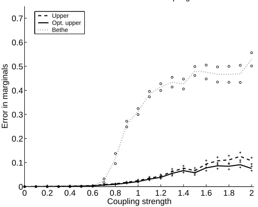
sta-ble—that is, even for very strongly coupled problems. For instance, Figure 2 provides a simple
illustration of the instability of the ordinary sum-product algorithm, contrasted with the stability of the tree-reweighted updates. Wiegerinck (2005) provides similar results for reweighted forms of the generalized belief propagation. Here we provide theoretical support for these empirical
observa-0 0.2 0.4 0.6 0.8 1 1.2 1.4 1.6 1.8 2 0
0.1 0.2 0.3 0.4 0.5 0.6 0.7
Coupling strength
Error in marginals
Grid with attractive coupling
Upper Opt. upper Bethe
Figure 2: Contrast of the instability of the ordinary sum-product algorithm with the stability of the tree-reweighted version (Wainwright et al., 2005). Results shown with a grid with
N=100 nodes over a range of attractive coupling strengths. The ordinary sum-product undergoes a phase transition, after which the quality of marginal approximations degrades substantially. The tree-reweighted algorithm, shown for two different settings of the edge weightsρst, remains stable over the full range of coupling strengths. See Wainwright
et al. (2005) for full details.
We begin by noting that for a multinomial Markov random field (3), the computation of the exact marginal probabilities is a globally Lipschitz operation:
Lemma 4 For any discrete Markov random field (3), there is a constant L<+∞such that
kµ(θ+δ)−µ(θ)k ≤ Lkδk for allθ,δ∈Rd.
This lemma, which is proved in Appendix B, guarantees that small changes in the problem pa-rameters—that is, “perturbations”δ—lead to correspondingly small changes in the computed mar-ginals.
Our goal is to establish analogous Lipschitz properties for variational methods. In particular, it turns out that any variational method based on a suitably concave entropy approximation satisfies such a stability condition. More precisely, a function f :Rn→Ris strongly convex if there exists a constant c>0 such that f(y)≥ f(x) +∇f(x)T y−x) +c
2ky−xk
2 for all x,y∈Rn. For a twice
continuously differentiable function, this condition is equivalent to having the eigenspectrum of the Hessian∇2f(x)be uniformly bounded below by c. With this definition, we have:
Proposition 5 Consider any strictly convex surrogate B based on a strongly concave entropy ap-proximation−B∗. Then there exists a constant R<+∞such that
kτ(θ+δ)−τ(θ)k ≤ Rkδk for allθ,δ∈Rd.
Proof From Proposition 2, we haveτ(θ) =∇B(θ), so that the statement is equivalent to the assertion that the gradient∇B is a Lipschitz function. Applying the mean value theorem to∇B, we can write
∇B(θ+δ)−∇B(θ) =∇2B(θ+tδ)δwhere t∈[0,1]. Consequently, in order to establish the Lipschitz
condition, it suffices to show that the spectral norm of∇2B(γ)is uniformly bounded above over all
γ∈Rd. Since B and B∗ are a strictly convex Legendre pair, we have ∇2B(θ) = [∇2B∗(τ(θ))]−1.
By the strong convexity of B∗, we are guaranteed that the spectral norm of ∇2B∗(τ)is uniformly bounded away from zero, which yields the claim.
A number of existing entropy approximations can be shown to be strongly concave. In Appendix C, we provide a detailed proof of this fact for the convexified Bethe entropy (12).
Lemma 6 For any set{ρst}of strictly positive edge appearance probabilities, the convexified Bethe entropy (12) is strongly concave.
6. Performance Bounds
In this section, we develop theoretical bounds on the performance loss of our approximate approach to joint estimation and prediction, relative to the unattainable Bayes optimum. So as not to unnec-essarily complicate the result, we focus on the performance loss in the infinite data limit2 (i.e., for which the number of samples n= +∞).
In the infinite data setting, the Bayes optimum is unattainable for two reasons:
1. it is based on knowledge of the exact parameterθ∗, which is not easy to obtain.
2. it assumes (in the prediction phase) that computing exact marginal probabilities µ of the Markov random field is feasible.
Of these two difficulties, it is the latter assumption—regarding the computation of marginal prob-abilities—that is the most serious. As discussed earlier, there do exist computationally tractable estimators ofθ∗ that are consistent though not statistically efficient under appropriate conditions; one example is the pseudolikelihood method (Besag, 1975, 1977) mentioned previously. On the other hand, MCMC methods may be used to generate stochastic approximations to marginal prob-abilities, but may require greater than polynomial complexity.
Recall from Proposition 3 that the parameter estimator based on the surrogate likelihood `B
is inconsistent, in the sense that the parameter vector bθ returned in the limit of infinite data is generally not equal to the true parameterθ∗. Our analysis in this section will demonstrate that this inconsistency is beneficial.
6.1 Problem Set-up
Although the ideas and techniques described here are more generally applicable, we focus here on a special observation model so as to obtain a concrete result.
Observation model: In particular, we assume that the multinomial random vector X ={Xs, s∈ V}defined by the Markov random field (3) is a label vector for the components in a finite mixture of Gaussians. For each node s∈V , we specify a new random variable Zsby the conditional distribution
p(Zs=zs|Xs= j)∼N(νj,σ2j) for j∈ {0,1, . . . ,m−1},
so that Zs is a mixture of m Gaussians. Such Gaussian mixture models are widely used in
spa-tial statistics as well as statistical signal and image processing (Crouse et al., 1998; Ripley, 1981; Titterington et al., 1986).
Now suppose that we observe a noise-corrupted version of zs—namely, a vector Y of
observa-tions with components of the form
Ys=αZs+
p
1−α2W
s, (21)
where Ws∼N(0,1)is additive Gaussian noise, and the parameterα∈[0,1]specifies the
signal-to-noise ratio (SNR) of the observation model. Note thatα=0 corresponds to pure noise, whereas
α=1 corresponds to completely uncorrupted observations.
Optimal prediction: Our goal is to compute an optimal estimatebz(y) of z as a function of the observation Y =y, using the mean-squared error as the risk function. The essential object in this
computation is the posterior distribution p(x | y ;θ∗)∝ p(x ;θ∗)p(y | x), where the conditional distribution p(y|x)is defined by the observation model (21). As shown in the sequel, the posterior distribution (with y fixed) can be expressed as an exponential family member of the formθ∗+γ(y) (see Equation (26a)). Disregarding computational cost, it is straightforward to show that the optimal Bayes least squares estimator (BLSE) takes the form
b
zopts (Y ;θ∗) :=
m−1
∑
j=0
µs; j(θ∗+γ(Y))
ωj(α) Ys−ανj+νj
, (22)
where µs; j(θ∗+γ) denotes the marginal probability associated with the posterior distribution p(x ;θ∗+γ), and
ωj(α) :=
ασ2 j α2σ2
j+ (1−α2)
(23)
is the usual BLSE weighting for a Gaussian with varianceσ2j.
Approximate prediction: Since the marginal distributions µs; j(θ∗+γ)are intractable to compute
exactly, it is natural to consider an approximate predictor, based on a set τ of pseudomarginals computed from a variational relaxation. More explicitly, we run the variational algorithm on the parameter vectorbθ+γthat is obtained by combining the new observation y with the fitted modelbθ, and use the outputted pseudomarginalsτs(·;bθ+γ)as weights in the approximate predictor
b
zapps (Y ;bθ) :=
m−1
∑
j=0
τs; j(bθ+γ(Y))
ωj(α) Ys−ανj+νj
, (24)
where the weightsωare defined in Equation (23).
We now turn to a comparison of the Bayes least-squares estimator (BLSE) defined in Equa-tion (22) to the surrogate-based predictor (24). Since (by definiEqua-tion) the BLSE is optimal for the mean-squared error (MSE), using the surrogate-based predictor will necessarily lead to a larger MSE. Our goal is to prove an upper bound on the maximal possible increase in this MSE, where the bound is specified in terms of the underlying modelθ∗and the SNR parameterα. More specifically, for a given problem, we define the mean-squared errors
Ropt(α,θ∗):= 1 NEkbz
opt(Y ;θ∗)−Zk2, and Rapp(α,bθ):= 1 NEkbz
app(Y ;bθ) −Zk2,
of the Bayes-optimal and surrogate-based predictors respectively, where the expectation is taken over the joint distribution of(Y,Z). We seek upper bounds on the increase∆R(α,θ∗,bθ):=Rapp(α,bθ) −Ropt(α,θ∗)of the approximate predictor relative to Bayes optimum.
6.2 Role of Stability
noise, so that the prediction of Z should be based simply on the estimated model—namely, the true model p(·;θ∗) in the Bayes optimal case, and the “incorrect” model p(·;bθ) for the method based on surrogate likelihood. The key point here is the following: by properties of the MLE and surrogate-based estimator, the following equalities hold:
∇A(θ∗) (=a) µ(θ∗) (=b) µ∗ (=c) τ(bθ) (=d) ∇B(bθ).
Here equality (a) follows from Lemma 1, whereas equality (b) follows from the moment-matching property of the MLE in exponential families. Equalities (c) and (d) hold from the Proposition 2 and the pseudomoment-matching property of the surrogate-based parameter estimator (see proof of Proposition 3). As a key consequence, it follows that the combination of surrogate-based estima-tion and predicestima-tion is funcestima-tionally indistinguishable from the Bayes-optimal behavior in the limit ofα=0. More specifically, in the limiting case, the errors systematically introduced by the in-consistent learning procedure are cancelled out exactly by the approximate variational method for computing marginal distributions. Of course, exactness for α=0 is of limited interest; however, when combined with the Lipschitz stability ensured by Proposition 5, it allows us to gain good con-trol of the low SNR regime. At the other extreme of high SNR (α≈1), the observations are nearly perfect, and hence dominate the behavior of the optimal estimator. More precisely, forαclose to 1, we haveωj(α)≈1 for all j=0,1, . . . ,m−1, so thatbzopt(Y ;θ∗)≈Y ≈bzapp(Y ;bθ). Consequently, in
the high SNR regime, accuracy of the marginal computation has little effect on the accuracy of the predictor.
6.3 Bound on Performance Loss
Although bounds of this nature can be developed in more generality, for simplicity in notation we focus here on the case of m=2 mixture components. We begin by introducing the factors that play a role in our bound on the performance loss∆R(α,θ∗,bθ). First, the Lipschitz stability enters in the form of the quantity:
L(θ∗;bθ) := sup
δ∈Rd
σmax ∇2A(θ∗+δ)−∇2B(bθ+δ), (25)
whereσmaxdenotes the maximal singular value. Following the argument in the proof of Proposi-tion 5, it can be seen that L(θ∗;bθ)is finite.
Second, in order to apply the Lipschitz stability result, it is convenient to express the effect of introducing a new observation vector y, drawn from the additive noise observation model (21), as a perturbation of the exponential parameterization. In particular, for any parameterθ∈Rd and observation y from the model (21), the conditional distribution p(x|y;θ)can be expressed as p(x;θ+ γ(y,α)), where the exponential parameterγ(y,α)has components3
γs =
1 2
( logα
2σ2
0+ (1−α2) α2σ2
1+ (1−α2)
+ (ys−αν0) 2 α2σ2
0+ (1−α2)
− (ys−αν1) 2 α2σ2
1+ (1−α2)
)
∀s∈V.(26a)
γst = 0 ∀(s,t)∈E. (26b)
See Appendix D for a derivation of these relations.
Third, it is convenient to have short notation for the Gaussian estimators of each mixture com-ponent:
gj(Ys;α) := ωj(α) (Ys−ανj) +νj for j=0,1,
With this notation, we have the following
Theorem 7 The MSE increase∆R(α,θ∗,bθ):=R(α,bθ)−R(α,θ∗)is upper bounded by
∆R(α,θ∗,bθ) ≤ E
min
1,L(θ∗;bθ)kγ(Y ;√α)k2 N
s∑N
s=1|g1(Ys)−g0(Ys)|4 N
. (27)
Before proving the bound (27), we illustrate it by considering its behavior in some special cases.
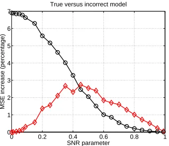
6.3.1 SUPERIORITY TOTRUEMODEL
Theorem 7 can be used to establish that applying an approximate message-passing algorithm to the “incorrect” model yields prediction results superior to those obtained by applying the same message-passing algorithm to the true underlying model. To see one regime in which this claim is true, consider the low SNR limit in whichα→0+. In this limit, it can be seen thatkγ(Y ;α)k →0, so that the the overall bound∆R(α)tends to zero. That is, the combination of approximate estimation and approximate prediction is asymptotically optimal in the low SNR limit. In sharp contrast, this claim need not be true when approximate prediction is applied to the true underlying model. As a particular example, consider a Gaussian mixture with m=2 components, with equal variances but distinct means (sayν0=−1 andν1=1). Moreover, suppose that the mixture indicator vectors
X∈ {0,1}N are sampled from an underlying distribution p(x;θ∗), and let µs= [µs;0µs;1]denote the
marginal distributions associated with this underlying model. In the limit of zero SNR (i.e.,α=0), it is straightforward to see that the BLSE of Z is simply its mean, given (for component s∈V ) by
E[Zs|Y] = E[Zs] = µs;0ν0+µs;1ν1 = µs;1−µs;0,
for the two-component mixture specified above. Now suppose that when applied to this true model,
the approximate message-passing algorithm yields an incorrect set of singleton pseudomarginals—
sayτs6=µs. Since standard message-passing algorithms are rarely (if ever) exactly correct on
non-trivial models with cycles, this assumption is more than reasonable. Consequently applying the approximate predictor to the true model will yield an estimate of Z which is incorrect, even in the zero SNR limit; in particular, the approximate estimate is given by
b
Z(Y ;θ∗) = τs;0ν0+τs;1ν1 = τs;1−τs;0 6= E[Z].
Thus, in contrast to the combination of approximate estimation with approximate estimation, apply-ing the approximate message-passapply-ing algorithm to the true model fails to be exact even in the limit of zero SNR. In fact, our later experimental results show that the superiority of using the “wrong” model holds for a broader range of SNRs as well (see Figure 4).
We conclude by turning to the high SNR limit asα→1−, in which we see thatωj(α)→1 for j=0,1, which drives the differences|g1(Ys)−g0(Ys)|, and in turn the overall bound∆R(α)to zero.
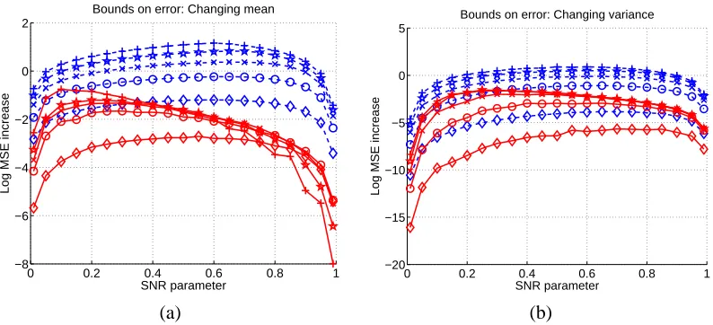
6.3.2 EFFECT OFEQUALVARIANCES
Now consider the special case of equal variancesσ2≡σ2
0=σ21, in which case ω(α)≡ω0(α) = ω1(α). Thus, the difference g1(Ys,α)−g0(Ys,α) simplifies to(1−αω(α)) (ν1−ν0), so that the
bound (27) reduces to
∆R(α,θ∗,bθ) ≤ (1−αω(α))2(ν1−ν0)2E
min
1,L(θ∗;bθ)kγ(Y ;√α)k2 N
. (28)
As shown by the simpler expression (28), forν1≈ν0, the MSE increase is very small, since such a two-component mixture is close to a pure Gaussian.
6.3.3 EFFECT OFMEAN DIFFERENCES
Finally consider the case of equal meansν≡ν0=ν1in the two Gaussian mixture components. In this case, we have g1(Ys,α)−g0(Ys,α) = [ω1(α)−ω0(α)] [Ys−αν], so that the bound (27) reduces
to
∆R(α,θ∗,bθ) ≤ [ω1(α)−ω0(α)]2 E
( min
1,L(θ∗;θb)kγ(Y ;α√ )k2 N
r∑
s(Ys−αν)4 N
)
.
Here the MSE increase depends on the SNRαand the difference
ω1(α)−ω0(α) = ασ 2 1 α2σ2
1+ (1−α2)
− ασ
2 0 α2σ2
0+ (1−α2)
= (1−α
2) (σ2 1−σ20)
α2σ2
0+ (1−α2) α2σ21+ (1−α2)
.
Observe, in particular, that the MSE increases tends to zero as the differenceσ21−σ20decreases, as should be expected intuitively.
6.4 Proof of Theorem 7
We now turn to the proof of the main bound (27). By the Pythagorean relation that characterizes the Bayes least squares estimatorbzopt(Y ;θ∗) =E(Z|Y,θ∗)[Z], we have
∆R(α;θ∗,bθ) := 1 NEkbz
app(Y ;bθ)−Zk2 2−
1
NEkbz
opt(Y ;θ∗)−Zk2 2
= 1
NEkbz
app(Y ;bθ)
−bzopt(Y ;θ∗)k22.
Using the definitions ofbzapp(Y ;bθ)andbzopt(Y ;θ∗), some algebraic manipulation yields h
bzapps (Y ;bθ)−bzopts (Y ;θ∗)i2 = hτs(bθ+γ)−µs(θ∗+γ)
i2
[g1(Ys)−g0(Ys)]2 ≤ τs(bθ+γ)−µs(θ∗+γ)
[g1(Ys)−g0(Ys)]2,
where the second inequality uses the fact that|τs−µs| ≤1 sinceτsand µsare marginal probabilities.
Next we write
1
Nkbz
app(Y ;bθ)
−bzopt(Y ;θ∗)k22 ≤ 1 N
N
∑
s=1
τs(bθ+γ)−µs(θ∗+γ)
[g1(Ys)−g0(Ys)]2 (29)
≤ √1
Nkτ(bθ+γ)−µ(θ
∗+γ)k
2
s
∑N
where the last line uses the Cauchy-Schwarz inequality.
It remains to bound the 2-normkτ(bθ+γ)−µ(θ∗+γ)k2. An initial naive bound follows from the factτs,µs∈[0,1]implies that|τs−µs| ≤1, whence
1
√
Nkτ−µk2≤ 1. (30)
An alternative bound, which will be better for small perturbations γ, can be obtained as follows. Using the relation τ(bθ) =µ(θ∗) guaranteed by the definition of the ML estimator and surrogate estimator, we have
kτ(bθ+γ)−µ(θ∗+γ)k2 = hτ(bθ+γ)−τ(bθ)i+ [µ(θ∗)−µ(θ∗+γ)] 2 = h∇2B(bθ+sγ)−∇2A(θ∗+tγ)iγ
2,
for some s,t∈[0,1], where we have used the mean value theorem. Thus, using the definition (25) of L, we have
1
√
N kτ(bθ+γ)−µ(θ
∗+γ)k2 ≤ L(θ∗;bθ)kγ(Y ;√α)k2
N . (31)
Combining the bounds (30) and (31) and applying them to Equation (29), we obtain
1
Nkbz
app(Y ;bθ)−bzopt(Y ;θ∗)k2
2 ≤ min
1,L(θ∗;bθ)kγ(Y ;√α)k2 N
s∑N
s=1|g1(Ys)−g0(Ys)|4
N .
Taking expectations of both sides yields the result.
7. Experimental Results
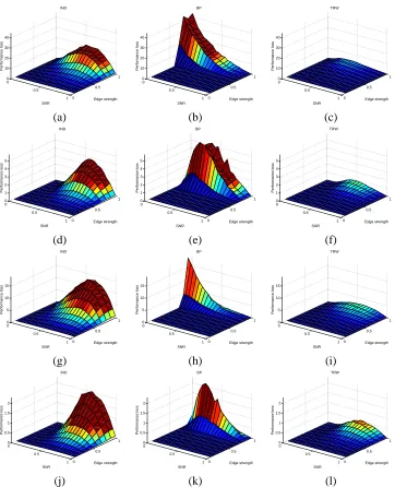
In order to test our joint estimation/prediction procedure, we have applied it to coupled Gaussian mixture models on different graphs, coupling strengths, observation SNRs, and mixture distribu-tions. Here we describe both experimental results to quantify the performance loss of the tree-reweighted sum-product algorithm (Wainwright et al., 2005), and compare it to both a baseline in-dependence model, as well as a closely related heuristic method that uses the ordinary sum-product (or belief propagation) algorithm.
7.1 Methods
In Section 4.2, we described a generic procedure for joint estimation and prediction. Here we begin by describing the special case of this procedure when the underlying variational method is the reweighted sum-product algorithm (Wainwright et al., 2005). Any instantiation of the tree-reweighted sum-product algorithm is specified by a collection of edge weightsρst, one for each
1. Given an initial set of i.i.d. data{X1, . . . ,Xn}, we first compute the empirical marginal distri-butions
bµs; j:=
1
n n
∑
i=1
I[Xsi=j], bµst; jk:=
1
n n
∑
i=1
I[Xsi= j]I[Xti=k],
and use them to compute the approximate parameter estimate
b
θn
s; j:=logbµs; j, θbns; j:=ρst log b µst; jk
bµs; jbµt;k
. (32)
As shown in our previous work (Wainwright et al., 2003b), the estimates (32) are the global maxima of the surrogate likelihood (16) based on the convexified Bethe approximation (12) without any regularization term (i.e., R=0).
2. Given the new noisy observation Y of the form (21), we incorporate it by by forming the new exponential parameter
b
θn
s+γs(Y),
where Equation (26a) definesγsfor the Gaussian mixture model under consideration.
3. We then compute approximate marginals τ(bθ+γ) by running the TRW sum-product algo-rithm with edge appearance weightsρst, using the message updates (14), on the graphical
model distribution with exponential parameterbθ+γ. We use the approximate marginals (see Equation (15)) to construct the predictionbzappin Equation (24).
We evaluated the tree-reweighted sum-product based on its increase in mean-squared error (MSE) over the Bayes optimal predictor (22). Moreover, we compared the performance of the tree-reweighted approach to the following alternatives:
(a) As a baseline, we used the independence model in which the mixture distributions at each node are all assumed to be independent. In this case, ML estimates of the parameters are given bybθs; j=logbµs; j, with all of the coupling termsbθst; jk equal to zero. The prediction step
reduces to computing the Bayes least squares estimate at each node independently, based only on the local data ys.
(b) The standard sum-product or belief propagation (BP) approach is closely related to the tree-reweighted sum-product method, but based on the edge weights ρst =1 for all edges. In
particular, we first form the approximate parameter estimatebθusing Equation (32) withρst=
1. As shown in our previous work (Wainwright et al., 2003b), this approximate parameter estimate uniquely defines the Markov random field for which the empirical marginalsbµsand
bµst are fixed points of the ordinary belief propagation algorithm. We note that a parameter
estimator of this type has been used previously by other researchers (Freeman et al., 2000; Ross and Kaebling, 2005). In the prediction step, we then use the ordinary belief propagation algorithm (i.e., again withρst=1) to compute approximate marginals of the graphical model
with parameterbθ+γ. Finally, based on these approximate BP marginals, we compute the approximate predictor using Equation (24).
Although our methods are more generally applicable, here we show representative results for
(a) Mixture ensemble A is bimodal, with components(ν0,σ2
0) = (−1,0.5)and(ν1,σ21) = (1,0.5).
(b) Mixture ensemble B was constructed with mean and variance components(ν0,σ2
0) = (0,1)
and(ν1,σ2
1) = (0,9); these choices serve to mimic heavy-tailed behavior.
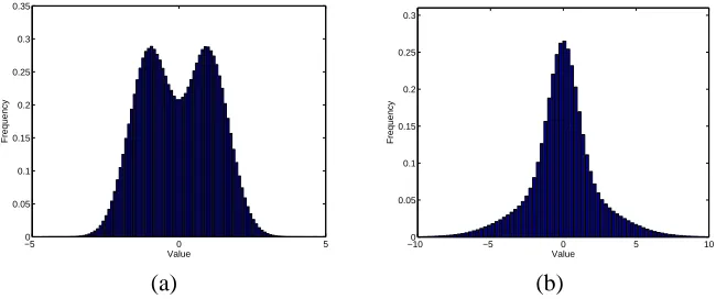
In both cases, each mixture component is equally weighted; see Figure 3 for histograms of the resulting mixture ensembles.
−5 0 5
0 0.05 0.1 0.15 0.2 0.25 0.3 0.35
Value
Frequency
−100 −5 0 5 10
0.05 0.1 0.15 0.2 0.25 0.3
Value
Frequency
(a) (b)
Figure 3: Histograms of different Gaussian mixture ensembles. (a) Ensemble A: a bimodal ensem-ble with(ν0,σ2
0) = (−1,0.5)and(ν1,σ21) = (1,0.5). (b) Ensemble B: mimics a
heavy-tailed distribution, with(ν0,σ2
0) = (0,1)and(ν1,σ21) = (0,9).
Here we show results for a 2-D grid with N=64 nodes. Since the mixture variables have m=2 states, the coupling distribution can be written as
p(x ;θ∗)∝exp
∑
s∈V θ∗
sxs+
∑
(s,t)∈E
θ∗
stxsxt ,
where x∈ {−1,+1}N are “spin” variables indexing the mixture components. In all trials (except
those in Section 7.2), we choseθ∗s =0 for all nodes s∈V , which ensures uniform marginal
dis-tributions p(xs;θ∗) = [0.5 0.5]T at each node. We tested two types of coupling in the underlying
Markov random field:
(a) In the case of attractive coupling, for each coupling strengthβ∈[0,1], we chose edge param-eters asθ∗st∼
U
[0,β].(b) In the case of mixed coupling, for each coupling strengthβ∈[0,1], we chose edge parameters asθ∗st∼
U
[−β,β].Here
U
[a,b]denotes a uniform distribution on the interval[a,b]. In all cases, we varied the SNR parameterα, as specified in the observation model (21), in the interval[0,1].7.2 Comparison between “Incorrect” and True Model