Fast SVM Training Using Approximate Extreme Points
Manu Nandan [email protected]
Department of Computer and Information Science and Engineering University of Florida
Gainesville, FL 32611, USA
Pramod P. Khargonekar [email protected]
Department of Electrical and Computer Engineering University of Florida
Gainesville, FL 32611, USA
Sachin S. Talathi [email protected]
Qualcomm Research Center 5775 Morehouse Dr
San Diego, CA 92121, USA
Editor:Sathiya Keerthi
Abstract
Applications of non-linear kernel support vector machines (SVMs) to large data sets is seriously hampered by its excessive training time. We propose a modification, called the approximate extreme points support vector machine (AESVM), that is aimed at overcoming this burden. Our approach relies on conducting the SVM optimization over a carefully selected subset, called the representative set, of the training data set. We present analytical results that indicate the similarity of AESVM and SVM solutions. A linear time algorithm based on convex hulls and extreme points is used to compute the representative set in kernel space. Extensive computational experiments on nine data sets compared AESVM to LIBSVM (Chang and Lin, 2011), CVM (Tsang et al., 2005) , BVM (Tsang et al., 2007), LASVM (Bordes et al., 2005), SVMperf (Joachims and Yu, 2009), and the random features method (Rahimi and Recht, 2007). Our AESVM implementation was found to train much faster than the other methods, while its classification accuracy was similar to that of LIBSVM in all cases. In particular, for a seizure detection data set, AESVM training was almost 500 times faster than LIBSVM and LASVM and 20 times faster than CVM and BVM. Additionally, AESVM also gave competitively fast classification times.
Keywords: support vector machines, convex hulls, large scale classification, non-linear kernels, extreme points
1. Introduction
time complexity for SVMs with non-linear kernels is typically quadratic in the size of the training data set (Shalev-Shwartz and Srebro, 2008). The difficulty of the long training time is exacerbated when grid search with cross-validation is used to derive the optimal hyper-parameters, since this requires multiple SVM training runs. Another problem that sometimes restricts the applicability of SVMs is the long classification time. The time complexity of SVM classification is linear in the number of support vectors and in some applications the number of support vectors is found to be very large (Guo et al., 2005).
In this paper, we propose a new approach for fast SVM training. Consider a two class data set ofN data vectors,X={xi: xi∈RD, i= 1,2, ..., N}, and the corresponding target
labelsY={yi : yi ∈[−1,1], i= 1,2, ..., N}. The SVM primal problem can be represented
as the following unconstrained optimization problem (Teo et al., 2010; Shalev-Shwartz et al., 2011):
min
w,b F1(w, b) =
1 2kwk
2+ C
N
N
X
i=1
l(w, b, φ(xi)), (1)
wherel(w, b, φ(xi)) =max{0,1−yi(wTφ(xi) +b)},∀xi∈X
and φ:RD →H, b∈R, andw∈H, a Hilbert space.
Here l(w, b, φ(xi)) is the hinge loss of xi. Note that SVM formulations where the penalty
parameterC is divided byN have been used extensively (Sch¨olkopf et al., 2000; Franc and Sonnenburg, 2008; Joachims and Yu, 2009). These formulations enable better analysis of the scaling of C with N (Joachims, 2006). The problem in (1) requires optimization over N variables. In general, for SVM training algorithms, the training time will reduce if the size of the training data set is reduced.
In this paper, we present an alternative to (1), called approximate extreme points support vector machines (AESVM), that requires optimization over only a subset of the training data set. The AESVM formulation is:
min
w,b F2(w, b) =
1 2kwk
2+ C
N
M
X
t=1
βtl(w, b, φ(xt)), (2)
where xt∈X∗,w∈H, and b∈R.
Here M is the number of vectors in the selected subset ofX, called the representative set
X∗. The constants βt are defined in (9). We will prove in Section 3.2 that:
• F1(w1∗, b∗1)−F2(w∗2, b∗2)≤C √
C, where (w∗1, b∗1) and (w∗2, b∗2) are the solutions of (1) and (2) respectively.
• Under the assumptions given in corollary 4, F1(w∗2, b∗2)−F1(w∗1, b∗1)≤2C √
C.
• The AESVM problem minimizes an upper bound of a low rank Gram matrix approx-imation of the SVM objective function.
reduction in size of the training set, AESVM is also observed to result in fast classification. Considering that the representative set will have to be computed several times if grid search is used to find the optimum hyper-parameter combination, we also propose fast algorithms to compute Z∗. In particular, we present an algorithm of time complexity O(N) and an alternative algorithm of time complexity O(N log2 NP) to compute Z∗, where P is a predefined large integer.
Our main contribution is the new AESVM formulation that can be used for fast SVM training. We develop and analyze our technique along the following lines:
• Theoretical: Theorems 1 and 2 and Corollaries 3 to 5 provide some theoretical basis for the use of AESVM as a computationally less demanding alternative to the SVM formulation.
• Algorithmic: The algorithm DeriveRS, described in Section 4, computes the represen-tative set in linear time.
• Experimental: Our extensive experiments on nine data sets of varying characteristics illustrate the suitability of applying AESVM to classification on large data sets.
This paper is organized as follows: in Section 2, we briefly discuss recent research on fast SVM training that is closely related to this work. Next, we provide the definition of the representative set and discuss properties of AESVM. In Section 4, we present efficient algorithms to compute the representative set and analyze its computational complexity. Section 5 describes the results of our computational experiments. We compared AESVM to the widely used LIBSVM library, core vector machines (CVM), ball vector machines (BVM), LASVM, SVMperf, and the random features method by Rahimi and Recht (2007). Our experiments used eight publicly available data sets and a data set on EEG from an animal model of epilepsy (Talathi et al., 2008; Nandan et al., 2010). We conclude with a discussion of the results of this paper in Section 6.
2. Related Work
Several methods have been proposed to efficiently solve the SVM optimization problem. SVMs require special algorithms, as standard optimization algorithms such as interior point methods (Boyd and Vandenberghe, 2004; Shalev-Shwartz et al., 2011) have large memory and training time requirements that make it infeasible for large data sets. In the following sections we discuss the most widely used strategies to solve the SVM optimization problem. We present a comparison of some of these methods to AESVM in Section 6. SVM solvers can be broadly divided into two categories as described below.
2.1 Dual Optimization
given below:
max
α L1(α) = N
X
i=1
αi−
1 2
N
X
i=1 N
X
j=1
αiαjyiyjK(xi,xj), (3)
subject to 0≤αi≤
C N and
N
X
i=1
αiyi= 0.
Here K(xi,xj) = φ(xi)Tφ(xj), is the kernel product (Sch¨olkopf and Smola, 2001) of the
data vectors xi and xj, and α is a vector of all variables αi. Solving the dual problem is
computationally simpler, especially for non-linear kernels and a majority of the SVM solvers use dual optimization. Some of the major dual optimization algorithms are discussed below.
Decomposition methods (Osuna et al., 1997) have been widely used to solve (3). These methods optimize over a subset of the training data set, called the ‘working set’, at each al-gorithm iteration. SVMlight(Joachims, 1999) and SMO (Platt, 1999) are popular examples of decomposition methods. Both these methods have a quadratic time complexity for linear and non-linear SVM kernels (Shalev-Shwartz and Srebro, 2008). Heuristics such as shrink-ing and cachshrink-ing (Joachims, 1999) enable fast convergence of decomposition methods and reduce their memory requirements. LIBSVM (Chang and Lin, 2011) is a very popular im-plementation of SMO. Adual coordinate descent(Hsieh et al., 2008) SVM solver computes the optimalα value by modifying one variable αi per algorithm iteration. Dual coordinate
descent SVM solvers, such as LIBLINEAR (Fan et al., 2008), have been proposed primarily for the linear kernel.
Approximations of the Gram matrix(Fine and Scheinberg, 2002; Drineas and Mahoney, 2005), have been proposed to increase training speed and reduce memory requirements of SVM solvers. The Gram matrix is theNxN square matrix composed of the kernel products K(xi,xj), ∀xi,xj ∈X. Training set selectionmethods attempt to reduce the SVM training time by optimizing over a selected subset of the training set. Several distinct approaches have been used to select the subset. Some methods use clustering based approaches (Pavlov et al., 2000) to select the subsets. In Yu et al. (2003), hierarchical clustering is performed to derive a data set that has more data vectors near the classification boundary than away from it. Minimum enclosing ball clustering is used in Cervantes et al. (2008) to remove data vectors that are unlikely to contribute to the SVM training. Random sampling of training data is another approach followed by approximate SVM solvers. Lee and Mangasarian (2001) proposed reduced support vector machines (RSVM), in which only a random subset of the training data set is used. Bordes et al. (2005) proposed the LASVM algorithm that uses active selectiontechniques to train SVMs on a subset of the training data set.
Bredensteiner, 2000) using core sets. However, there are no published results on solving L1-SVM with non-linear kernels using their algorithm.
Another method used to approximately solve the SVM problem is to map the data vectors into a randomized feature space that is relatively low dimensional compared to the kernel space H (Rahimi and Recht, 2007). Inner products of the projections of the data
vectors are approximations of their kernel product. This effectively reduces the non-linear SVM problem into the simpler linear SVM problem, enabling the use of fast linear SVM solvers. This method is referred as RfeatSVM in the following sections of this document.
2.2 Primal Optimization
In recent years, linear SVMs have found increased use in applications with high-dimensional data sets. This has led to a surge in publications on efficient primal SVM solvers, which are mostly used for linear SVMs. To overcome the difficulties caused by the non-differentiability of the primal problem, the following methods are used.
Stochastic sub-gradient descent (Zhang, 2004) uses the sub-gradient computed at some data vector xi to iteratively updatew. Shalev-Shwartz et al. (2011) proposed a stochastic
sub-gradient descent SVM solver, Pegasos, that is reported to be among the fastest linear SVM solvers. Cutting plane algorithms (Kelley, 1960) solve the primal problem by succes-sively tightening a piecewise linear approximation. It was employed by Joachims (2006) to solve linear SVMs with their implementation SVMperf. This work was generalized in Joachims and Yu (2009) to include non-linear SVMs by approximately estimatingw with arbitrary basis vectors using the fix-point iteration method (Sch¨olkopf and Smola, 2001). Teo et al. (2010) proposed a related method for linear SVMs, that corrected some stability issues in the cutting plane methods.
3. Analysis of AESVM
As mentioned in the introduction, AESVM is an optimization problem on a subset of the training data set called the representative set. In this section we first define the representa-tive set. Then we present some properties of AESVM. These results are intended to provide theoretical justifications for the use of AESVM as an approximation to the SVM problem (1).
3.1 Definition of the Representative Set
The convex hull of a set Xis the smallest convex set containing X (Rockafellar, 1996) and can be obtained by taking all possible convex combinations of elements of X. AssumingX
is finite, the convex hull is a polygon. The extreme points ofX,EP(X), are defined to be the vertices of the convex polygon formed by the convex hull ofX. Any vectorxi inXcan be represented as a convex combination of vectors inEP(X):
xi =
X
xt∈EP(X)
πi,txt, where 0≤πi,t≤1, and
X
xt∈EP(X)
πi,t = 1.
intuition that the use of extreme points may provide computational efficiency. However, extreme points are not useful in all cases, as for some kernels all data vectors are extreme points in kernel space. For example, for the Gaussian kernel,K(xi,xi) =φ(xi)Tφ(xi) = 1.
This implies that all the data vectors lie on the surface of the unit ball in the Gaussian kernel space1 and therefore are extreme points. Hence, we introduce the concept of approximate extreme points.
Consider the set of transformed data vectors:
Z={zi :zi =φ(xi),∀xi∈X}. (4)
Here, the explicit representation of vectors in kernel space is only for the ease of under-standing and all the computations are performed using kernel products. LetV be a positive integer that is much smaller thanN and be a small positive real number. For notational simplicity, we assume N is divisible by V. Let Zl be subsets of Zfor l= 1,2, ...,(NV ), such
that Z = ∪
lZl and Zl∩Zm = ∅ for l 6= m, where m = 1,2, ...,( N
V). We require that the
subsets Zl satisfy|Zl|=V,∀l and
∀zi,zj ∈Zl, we have yi=yj, (5)
where |Zl| denotes the cardinality of Zl. Let Zlq be an arbitrary subset of Zl, Zlq ⊆ Zl.
Next, for any zi∈Zl we define:
f(zi,Zlq) =min
µi
kzi− X
zt∈Zlq
µi,tztk2, (6)
s.t. 0≤µi,t ≤1, and
X
zt∈Zlq
µi,t= 1.
A subset Zl∗ is said to be an- approximate extreme points subset of Zl if:
max
zi∈Zl
f(zi, Zl∗)≤.
We will drop the prefixfor simplicity and refer toZl∗as approximate extreme points subset. Note that it is not unique. Intuitively, its cardinality will be related to computational savings obtained using the approach proposed in this paper. We have chosen to not use approximate extreme points subset of smallest cardinality to maintain flexibility.
It can be seen that µi,t for zt ∈ Z∗l are analogous to the convex combination weights
πi,t forxt∈EP(X). The representative setZ∗ ofZis the union of the sets of approximate
extreme points of its subsets Zl.
Z∗=
N V
∪ l=1Z
∗ l.
The representative set has properties that are similar to EP(X). Given anyzi∈Z, we can find Zl such that zi ∈ Zl. Let γi,t ={µi,t forzt ∈ Z∗l and zi ∈ Zl, and 0 otherwise}.
Now using (6), we can write:
zi =
X
zt∈Z∗
γi,tzt+τi. (7)
Hereτi is a vector that accounts for the approximation errorf(zi,Zlq) in (6). From (6) and
(7) we can conclude that:
kτik2≤∀zi∈Z. (8)
Since will be set to a very small positive constant, we can infer that τi is a very small
vector. The weightsγi,t are used to defineβt in (2) as:
βt= N
X
i=1
γi,t. (9)
For ease of notation, we refer to the set X∗ := {xt : zt ∈ Z∗} as the representative set of X in the remainder of this paper. For the sake of simplicity, we assume that all γi,t, βt,X, and X∗ are arranged so thatX∗ is positioned as the firstM vectors ofX, where
M =|Z∗|.
3.2 Properties of AESVM
Consider the following optimization problem.
min
w,b F3(w, b) =
1 2kwk
2 + C
N
N
X
i=1
l(w, b,ui), (10)
whereui=
M
X
t=1
γi,tzt,zt∈Z∗,w∈H, and b∈R.
We use the problem in (10) as an intermediary between (1) and (2). The intermediate problem (10) has a direct relation to the AESVM problem, as given in the following theorem. The properties of themax function given below are relevant to the following discussion:
max(0, A+B)≤max(0, A) +max(0, B), (11)
max(0, A−B)≥max(0, A)−max(0, B), (12)
N
X
i=1
max(0, ciA) =max(0, A) N
X
i=1
ci, (13)
forA, B, ci ∈R andci ≥0.
Theorem 1 Let F3(w, b) and F2(w, b) be as defined in (10) and (2) respectively. Then,
Proof Let L2(w, b,X∗) = NC
M
P
t=1
l(w, b,zt) N
P
i=1
γi,t and L3(w, b,X∗) = NC N
P
i=1
l(w, b,ui), where
ui = M
P
t=1
γi,tzt. From the properties ofγi,t in (6), and from (5) we get:
L3(w, b,X∗) = C N N X i=1 max " 0, (
1−yi(wT M
X
t=1
γi,tzt+b)
)# = C N N X i=1 max " 0, M X t=1 γi,t
1−yt(wTzt+b)
#
.
Using properties (11) and (13) we get:
L3(w, b,X∗)≤ C
N N X i=1 M X t=1 max
0, γi,t
1−yt(wTzt+b)
= C N
M
X
t=1
max0,1−yt(wTzt+b)
N
X
i=1
γi,t
=L2(w, b,X∗).
Adding 12kwk2 to both sides of the inequality above we get F3(w, b)≤F2(w, b).
The following theorem gives a relationship between the SVM problem and the interme-diate problem.
Theorem 2 Let F1(w, b) and F3(w, b) be as defined in (1) and (10) respectively. Then,
− C
N
N
X
i=1
max0, yiwTτi ≤F1(w, b)−F3(w, b)≤
C N
N
X
i=1
max0,−yiwTτi ,
∀w∈Hand b∈R, where τi ∈His the vector defined in (7).
Proof Let L1(w, b,X) = NC
N
P
i=1
l(w, b,zi), denote the average hinge loss that is minimized
in (1) andL3(w, b,X∗) be as defined in Theorem 1. Using (7) and (1) we get:
L1(w, b,X) = C N
N
X
i=1
max
0,1−yi(wTzi+b)
= C N N X i=1 max (
0,1−yi(wT( M
X
t=1
γi,tzt+τi) +b)
)
From the properties of γi,t in (6), and from (5) we get:
L1(w, b,X) =
C N N X i=1 max ( 0, M X t=1
γi,t(1−yt(wTzt+b))−yiwTτi
)
. (14)
Using (11) on (14), we get:
L1(w, b,X)≤
C N N X i=1 max " 0, M X t=1 γi,t
1−yt(wTzt+b)
# + C N N X i=1 max
0,−yiwTτi
=L3(w, b,X∗) +
C N
N
X
i=1
max0,−yiwTτi .
Using (12) on (14), we get:
L1(w, b,X)≥
C N N X i=1 max " 0, M X t=1 γi,t
1−yt(wTzt+b)
# − C N N X i=1
max0, yiwTτi
=L3(w, b,X∗)− C
N
N
X
i=1
max
0, yiwTτi .
From the two inequalities above we get,
L3(w, b,X∗)−
C N
N
X
i=1
max0, yiwTτi ≤ L1(w, b,X)
≤ L3(w, b,X∗) +
C N N X i=1 max
0,−yiwTτi .
Adding 12kwk2 to the inequality above we get
F3(w, b)−
C N
N
X
i=1
max0, yiwTτi ≤F1(w, b)≤F3(w, b) +
C N
N
X
i=1
max0,−yiwTτi .
Using the above theorems we derive the following corollaries. These results provide the theoretical justification for AESVM.
Corollary 3 Let (w∗1, b∗1) be the solution of (1) and (w2∗, b∗2) be the solution of (2). Then,
F1(w∗1, b ∗
1)−F2(w2∗, b ∗ 2)≤C
√
Proof It is known that kw1∗k ≤ √C (see Shalev-Shwartz et al., 2011, Theorem 1). It is straight forward to see that the same result also applies to AESVM, kw∗2k ≤√C . Based on (8) we know thatkτik ≤
√
. From Theorem 2 we get:
F1(w∗2, b∗2)−F3(w∗2, b∗2)≤
C N N X i=1 max
0,−yiw2∗Tτi ≤
C N
N
X
i=1
kw2∗kkτik
≤ C N N X i=1 √
C=C
√
C.
Since (w∗1, b∗1) is the solution of (1), F1(w∗1, b∗1) ≤ F1(w∗2, b∗2). Using this property and
Theorem 1 in the inequality above, we get:
F1(w∗1, b∗1)−F2(w∗2, b∗2)≤F1(w1∗, b∗1)−F3(w∗2, b∗2) ≤F1(w2∗, b∗2)−F3(w∗2, b∗2)≤C
√
C.
Now we demonstrate some properties of AESVM using the dual problem formulations of AESVM and the intermediate problem. The dual form of AESVM is given by:
max
ˆ
α L2( ˆα) = M
X
t=1
ˆ αt−
1 2 M X t=1 M X s=1 ˆ
αtαˆsytyszTtzs, (15)
subject to 0≤αˆt≤
C N
N
X
i=1
γi,t and M
X
t=1
ˆ
αtyt= 0.
The dual form of the intermediate problem is given by:
max ˘
α L3( ˘α) = N
X
i=1
˘ αi−
1 2 N X i=1 N X j=1 ˘
αiα˘jyiyjuTi uj, (16)
subject to 0≤α˘i ≤
C N and N X i=1 ˘
αiyi = 0.
Consider the mapping function h:RN →RM, defined as
h( ˘α) ={α˜t: ˜αt= N
X
i=1
γi,tα˘i}. (17)
It can be seen that the objective functionsL2(h( ˘α)) andL3( ˘α) are identical.
L2(h( ˘α)) = M
X
t=1
˜ αt−
1 2 M X t=1 M X s=1 ˜
αtα˜sytyszTtzs
=
N
X
i=1
˘ αi−
1 2 N X i=1 N X j=1 ˘
αiα˘jyiyjuTi uj
It is also straight forward to see that, for any feasible ˘α of (16), h( ˘α) is a feasible point of (15) as it satisfies the constraints in (15). However, the converse is not always true. With that clarification, we present the following corollary.
Corollary 4Let (w∗1, b∗1) be the solution of (1) and(w∗2, b∗2) be the solution of (2). Letαˆ2 be the dual variable corresponding to (w∗2, b∗2). Let h( ˘α2) be as defined in (17). If there exists anα˘2 such that h( ˘α2) = ˆα2 and α˘2 is a feasible point of (16), then,
F1(w∗2, b∗2)−F1(w1∗, b∗1)≤2C √
C.
Proof Let (w3∗, b∗3) be the solution of (10) and ˘α3 the solution of (16). We know that
L3( ˘α2) =L2( ˆα2) =F2(w2∗, b∗2) and L3( ˘α3) =F3(w∗3, b∗3). Since L3( ˘α3)≥L3( ˘α2), we get
F3(w∗3, b ∗
3)≥F2(w∗2, b ∗ 2).
But, from Theorem 1 we knowF3(w∗3, b3∗)≤F3(w2∗, b∗2)≤F2(w∗2, b∗2). Hence
F3(w∗3, b∗3) =F3(w∗2, b∗2).
From the above result we get
F3(w∗2, b∗2)−F3(w1∗, b∗1)≤0. (18)
From Theorem 2 we have the following inequalities:
−C
N
N
X
i=1
max0, yiw∗T1 τi ≤F1(w∗1, b ∗
1)−F3(w∗1, b ∗
1), and (19)
F1(w∗2, b∗2)−F3(w∗2, b∗2)≤
C N N X i=1 max
0,−yiw2∗Tτi . (20)
Adding (19) and (20) we get:
F1(w∗2, b∗2)−F1(w∗1, b∗1)≤R+
C N N X i=1 max
0,−yiw∗T2 τi +max
0, yiw1∗Tτi , (21)
whereR=F3(w∗2, b∗2)−F3(w∗1, b∗1). Using (18) and the propertieskw2∗k ≤ √
C andkw∗1k ≤ √
C in (21) we get
F1(w2∗, b ∗
2)−F1(w∗1, b ∗ 1)≤
C N N X i=1
max0,−yiw∗T2 τi +max
0, yiw∗T1 τi
≤ C
N
N
X
i=1
kw∗2kkτik+kw∗1kkτik
≤ C N N X i=1 2 √
C= 2C
√
Now we prove a relationship between AESVM and the Gram matrix approximation methods mentioned in Section 2.1.
Corollary 5 Let L1(α), L3( ˘α), and F2(w, b) be the objective functions of the SVM dual (3), intermediate dual (16) and AESVM (2) respectively. Let zi, τi, and ui be as defined in (4), (7), and (10) respectively. Let Gand G˜ be the NxN matrices with Gij =yiyjzTi zj and G˜ij =yiyjuiTuj respectively. Then for any feasible α, α,˘ w,and b:
1. Rank of G˜ =M, L1(α) = N
P
i=1
αi−12αGαT, L3( ˘α) = N
P
i=1
˘
αi−12α˘G˜α˘T, and
Trace(G−G˜)≤N + 2
M
X
t=1 zTt
N
X
i=1
γi,tτi.
2. F2(w, b)≥L3( ˘α).
Proof UsingG, the SVM dual objective functionL1(α) can be represented as:
L1(α) = N
X
i=1
αi−
1 2αGα
T.
Similarly, L3( ˘α) can be represented using ˜Gas:
L3( ˘α) = N
X
i=1
˘ αi−
1 2α˘
˜
Gα˘T.
Applying ui = M
P
t=1
γi,tzt, ∀zt∈Z∗ to the definition of ˜G, we get:
˜
G= ΓAΓT.
Here Ais the MxM matrix comprised of Ats=ytyszTtzs, ∀zt,zs∈Z∗ and Γ is theNxM matrix with the elements Γit = γi,t. Hence the rank of ˜G = M and intermediate dual
problem (16) is a low rank approximation of the SVM dual problem (3).
The Gram matrix approximation error can be quantified using (7) and (8) as:
Trace(G−G˜) =
N
X
i=1
"
zTi zi−( M
X
t=1
γi,tzt)T( M
X
s=1
γi,szs)
# = N X i=1 "
τiTτi+ 2 M
X
t=1
γi,tzTtτi
#
≤N + 2
M
X
t=1 zTt
N
X
i=1
γi,tτi.
By the principle of duality, we know that F3(w, b)≥L3( ˘α), ∀w∈Hand b∈R, where
˘
α is any feasible point of (16). Using Theorem 1 on the inequality above, we get
Thus the AESVM problem minimizes an upper boundF2(w, b), of a rank M Gram matrix
approximation of L1(α).
Based on the theoretical results in this section, it is reasonable to suggest that for small values of, the solution of AESVM is close to the solution of SVM.
4. Computation of the Representative Set
In this section, we present algorithms to compute the representative set. The AESVM formulation can be solved with any standard SVM solver such as SMO and hence we do not discuss methods to solve it. As described in Section 3.1, we require an algorithm to compute approximate extreme points in kernel space. Osuna and Castro (2002) proposed an algorithm to derive extreme points of the convex hull of a data set in kernel space. Their algorithm is computationally intensive, with a time complexity of O(N S(N)), and is unsuitable for large data sets asS(N) typically has a super-linear dependence on N. The functionS(N) denotes the time complexity of a SVM solver (required by their algorithm), to train on a data set of size N. We next propose two algorithms leveraging the work by Osuna and Castro (2002) to compute the representative set in kernel space Z∗ with much smaller time complexities.
We followed the divide and conquer approach to develop our algorithms. The data set is first divided into subsets Xq, q = 1,2, .., Q, where |Xq| < P, Q ≥ NP and X = {X1,X2, ..,XQ}. The parameter P is a predefined large integer. It is desired that each subset Xq contains data vectors that are more similar to each other than data vectors in
other subsets. Our notion of similarity of data vectors in a subset, is that the distances be-tween data vectors within a subset is less than the distances bebe-tween data vectors in distinct subsets. Since performing such a segregation is computationally expensive, heuristics are used to greatly simplify the process. Instead of computing the distance of all data vectors from each other, only the distance from a few selected data vectors are used to segregate the data in the methods FLS2 and SLS described below.
The first level of segregation is followed by another level of segregation. We can regard the first level of segregation as coarse segregation and the second as fine segregation. Finally, the approximate extreme points of the subsets obtained after segregation, are computed. The two different algorithms to compute the representative set differ only in the first level of segregation as described below.
4.1 First Level of Segregation
We propose the methods, FLS1 and FLS2 given below to perform a first level of segregation. In the following description we use arrays ∆0 and ∆02 of N elements. Each element of ∆0 (∆02), δi (δ2i) , contains the index in X of the last data vector of the subset to which xi
belongs. It is straight forward to replace this N element array with a smaller array of size equal to the number of subsets. We use aN element array for ease of description. The set
X0 denotes any set of data vectors.
For some applications, such as anomaly detection on sequential data, data vectors are found to be homogeneous within intervals. For example, the atmospheric conditions typi-cally do not change within a few minutes and hence weather data is homogeneous for a short span. For such data sets it is enough to segregate the data vectors based on its position in the training data set. The same method can also be used on very large data sets without any homogeneity, in order to reduce computation time. The complexity of this method is O(N0), where N0 =|X0|.
[X0,∆0] = FLS1(X0, P)
1. For outerIndex = 1 to ceiling(|XP0|)
2. For innerIndex = (outerIndex - 1)P to min((outerIndex)P,|X0|) 3. SetδinnerIndex =min((outerIndex)P,|X0|)
2. FLS2(X0, P)
When the data set is not homogeneous within intervals or it is not excessively large we use the more sophisticated algorithm, FLS2, of time complexityO(N0 log2NP0) given below. In step 1 of FLS2, the distance di in kernel space of all xi ∈ X0 from xj is computed as
di =kφ(xi)−φ(xj)k2 =k(xi,xi) +k(xj,xj)−2k(xi,xj). The algorithm FLS2(X0, P), in
effect builds a binary search tree, with each node containing the data vectorxk selected in
step 2 that partitions a subset of the data set into two. The size of the subsets successively halve, on downward traversal from the root of the tree to the other nodes. When the size of all the subsets at a level become≤P the algorithm halts. The complexity of FLS2 can be derived easily when the algorithm is considered as an incomplete binary search tree building method. The last level of such a tree will have O(NP0) nodes and consequently the height of the tree isO(log2NP0). At each level of the tree the calls to the BFPRT algorithm (Blum et al., 1973) and the rearrangement of the data vectors in steps 2 and 3 are of O(N0) time complexity. Hence the overall time complexity of FLS2(X0, P) is O(N0 log2NP0).
4.2 Second Level of Segregation
After the initial segregation, another method SLS(X0, V,∆0) is used to further segregate each setXq into smaller subsetsXqr of maximum size V,Xq={Xq1,Xq2, ....,XqR}, whereV is
predefined (V < P) and R =ceiling(|XVq|). The algorithm SLS(X0, V,∆0) is given below. In step 2.b, xt is the data vector inXq that is farthest from the origin in the space of the
data vectors. For some kernels, such as the Gaussian kernel, all data vectors are equidistant from the origin in kernel space. If the algorithm choosesal in step 2.b based on distances in
[X0,∆0] = FLS2(X0, P)
1. Compute distance di in kernel space of allxi ∈X0 from the first vector xj inX0
2. Select xk such that there exists |X20| data vectors xi ∈ X0 with di < dk, using the
linear time BFPRT algorithm
3. Using xk, rearrange X0 as X0 = {X1,X2}, where X1 = {xi :di < dk,xi ∈ X0} and X2 ={xi :xi∈X0 and xi6∈X1}
4. If |X20| ≤P
Foriwhere xi∈X1, setδi = index of last data vector in X1.
Foriwhere xi∈X2, setδi = index of last data vector in X2.
5. If |X20| > P
Run FLS2(X1, P) and FLS2(X2, P)
complexity of SLS(X0, V,∆0) considering the Q For loop iterations is O(NP0PV2) ⇒O(NV0P), sinceQ=O(NP0).
[X0,∆02] = SLS(X0, V,∆0) 1. Initialize l= 1
2. For q = 1to Q
(a) Identify subsetXq ofX0 using ∆0
(b) Setal=φ(xt), where xt∈argmax i
kxik2,xi ∈Xq
(c) Compute distance di in kernel space of allxi ∈Xq fromal
(d) Selectxk such that, there exists V data vectors xi ∈Xq withdi < dk, using the
BFPRT algorithm
(e) Usingxk, rearrange Xq as Xq ={X1,X2}, where X1 ={xi :di < dk,xi ∈Xq}
and X2 ={xi :xi∈Xq and xi 6∈X1}
(f) Foriwherexi ∈X1, setδi2 = index of last data vector inX1, whereδi2 is theith
element of ∆02 (g) RemoveX1 from Xq
(h) If|X2|> V
Set: l=l+ 1 and al=xk
Repeat steps 2.c to 2.h
(i) If |X2| ≤V
4.3 Computation of the Approximate Extreme Points
After computing the subsetsXqr, the algorithm DeriveAE is applied to eachXqr to compute
its approximate extreme points. The algorithm DeriveAE is described below. DeriveAE uses three routines. SphereSet(Xqr) returns all xi ∈Xqr that lie on the surface of the smallest
hypersphere in kernel space that contains Xqr. It computes the hypersphere as a hard
margin support vector data descriptor (SVDD) (Tax and Duin, 2004). SphereSort(Xqr)
returns data vectors xi ∈ Xqr sorted in descending order of distance in the kernel space
from the center of the SVDD hypersphere. CheckPoint(xi,Ψ) returns TRUE if xi is an
approximate extreme point of the set Ψ in kernel space. The operator A\B indicates a set operation that returns the set of the members of A excluding A∩B. The matrix X∗qr
contains the approximate extreme points ofXqr and βqr is a|X
∗
qr|sized vector.
[X∗qr, βqr] = DeriveAE(Xqr)
1. Initialize: X∗qr = SphereSet(Xqr) and Ψ =∅
2. Setζ = SphereSort(Xqr\X
∗ qr)
3. For eachxi taken in order fromζ, call the routine CheckPoint(xi,X∗qr ∪Ψ)
If it returnsF ALSE, then set Ψ = Ψ∪xi
4. Initialize a matrix Γ of size |Xqr|x|X
∗
qr|with all elements set to 0
Setµk,k = 1∀xk ∈X∗qr, where µi,j is the element in the i
th row and jth column
of Γ
5. For eachxi ∈Xqr and xi 6∈X
∗
qr, execute CheckPoint(xi,X
∗ qr)
Set theith row of Γ = µi, whereµi is the result of CheckPoint(xi,X∗qr)
6. For j = 1 to |X∗qr|
Setβqjr =
|Xqr|
P
k=1
µk,j
CheckPoint(xi,Ψ) is computed by solving the following quadratic optimization problem:
min µi
p(xi,Ψ) =kφ(xi)− |Ψ|
X
t=1
µi,tφ(xt)k2,
s.t. xt∈Ψ,0≤µi,t ≤1 and |Ψ|
X
t=1
µi,t = 1,
wherekφ(xi)− |Ψ|
P
t=1
µi,tφ(xt)k2=K(xt,xt) + |Ψ|
P
t=1 |Ψ|
P
s=1
µi,tµi,sK(xt,xs)−2 |Ψ|
P
t=1
µi,tK(xi,xt). If the
optimized value of p(xi,Ψ)≤, CheckPoint(xi,Ψ) returns TRUE and otherwise it returns
FALSE. It can be seen that the formulation of p(xi,Ψ) is similar to (6). The value of µi
Now we compute the time complexity of DeriveAE. We use the fact that the opti-mization problem in CheckPoint(xi,Ψ) is essentially the same as the dual optimization problem of SVM given in (3). Since DeriveAE solves several SVM training problems in steps 1,3, and 5, it is necessary to know the training time complexity of a SVM. As any SVM solver method can be used, we denote the training time complexity of each step of DeriveAE that solves an SVM problem as O(S(Aqr)). Here Aqr is the largest value
of X∗qr ∪Ψ during the run of DeriveAE(Xqr). This enables us to derive a generic
ex-pression for the complexity of DeriveAE, independent of the SVM solver method used. Hence the time complexity of step 1 is O(S(Aqr)). The time complexity of steps 3 and
5 are O(V S(Aqr)) and O(Aqr S(Aqr)) respectively. The time complexity of step 2 is
O(V |Ψ1|+V log2V), where Ψ1 = SphereSet(Xqr). Hence the time complexity of
De-riveAE isO(V |Ψ1|+V log2V+V S(Aqr). Since |Ψ1|is typically very small, we denote the
time complexity of DeriveAE byO(V log2V+V S(Aqr)). For SMO based implementations
of DeriveAE, such as the implementation we used for Section 5, typicallyS(Aqr) =O(A
2 qr).
4.4 Combining All the Methods to Compute X∗
To derive X∗, it is required to first rearrange X, so that data vectors from each class are grouped together as X = {X+,X−}. Here X+ = {x
i : yi = 1,xi ∈ X}and X− = {xi : yi = −1,xi ∈ X}. Then the selected segregation methods are run on X+ and X− separately. The algorithm DeriveRS given below, combines all the algorithms defined earlier in this section with a few additional steps, to compute the representative set of
X. The complexity of DeriveRS2 can easily be computed by summing the complexities of its steps. The complexity of steps 1 and 6 is O(N). The complexity of step 2 is O(N) if FLS1 is run or O(N log2NP) if FLS2 is run. In step 3, the O(N PV ) method SLS is run. In steps 4 and 5, DeriveAE is run on all the subsets Xqr giving a total complexity of
O(N log2V +V
Q
P
q=1 R
P
r=1
S(Aqr)). Here we use the fact that the number of subsets Xqr is
O(NV). Thus the complexity of DeriveRS isO(N(PV + log2V) +V
Q
P
q=1 R
P
r=1
S(Aqr)) when FLS1
is used and O(N(log2NP +PV + log2V) +V
Q
P
q=1 R
P
r=1
S(Aqr)) when FLS2 is used.
5. Experiments
We focused our experiments on an SMO (Fan et al., 2005) based implementation of AESVM and DeriveRS. We evaluated the classification performance of AESVM using the nine data sets, described below. Next, we present an evaluation of the algorithm DeriveRS, followed by an evaluation of AESVM.
[X∗,Y∗, β] = DeriveRS(X,Y,P,V)
1. SetX+={xi:xi∈X, yi = 1} and X−={xi :xi ∈X, yi=−1}
2. Run [X+,∆+] = FLS(X+,P) and [X−,∆−] = FLS(X−,P), where FLS is FLS1 or FLS2
3. Run [X+,∆+2] = SLS(X+,V,∆+) and [X−,∆−2] = SLS(X−,V,∆−) 4. Using ∆+2, identify each subset Xqr of X
+ and run [X∗
qr, βqr] = DeriveAE(Xqr)
SetN+∗= sum of number of data vectors in all X∗qr derived fromX+
5. Using ∆−2, identify each subset Xqr of X
− and run [X∗
qr, βqr] = DeriveAE(Xqr)
SetN−∗= sum of number of data vectors in all X∗qr derived fromX−
6. Combine in the same order, all X∗qr to obtain X∗ and allβqr to obtain β
Set Y∗ = {yi : yi = 1 for i = 1,2, .., N+∗; and yi = −1 for i = 1 +N+∗,2 +
N+∗, .., N−∗+N+∗}
5.1 Data Sets
Nine data sets of varied size, dimensionality and density were used to evaluate DeriveRS and our AESVM implementation. For data sets D2, D3 and D4, we performed five fold cross validation. We did not perform five fold cross-validation on the other data sets, because they have been widely used in their native form with a separate training and testing set.
D1 KDD’99 intrusion detection data set:3 This data set is available as a training set of 4898431 data vectors and a testing set of 311027 data vectors, with forty one features (D = 41). As described in Tavallaee et al. (2009), a huge portion of this data set is comprised of repeated data vectors. Experiments were conducted only on the distinct data vectors. The number of distinct training set vectors wasN = 1074974 and the number of distinct testing set vectors was N = 77216. The training set density = 33%.
D2 Localization data for person activity:4 This data set has been used in a study on agent-based care for independent living (Kaluˇza et al., 2010). It hasN = 164860 data vectors of seven features. It is comprised of continuous recordings from sensors attached to five people and can be used to predict the activity that was performed by each person at the time of data collection. In our experiments we used this data set to validate a binary problem of classifying the activities ‘lying’ and ‘lying down’ from the other activities. Features 3 and 4, that gives the time information, were not used in our experiments. Hence for this data setD= 5. The data set density = 96%.
3. D1 is available for download athttp://archive.ics.uci.edu/ml/datasets/KDD+Cup+1999+Data. 4. D2 is available for download athttp://archive.ics.uci.edu/ml/datasets/Localization+Data+for+
D3 Seizure detection data set: This data set has N = 982863 data vectors, three features (D= 3) and density = 100%. It is comprised of continuous EEG recordings from rats induced with status epilepticus and is used to evaluate algorithms that classify seizure events from seizure-free EEG. An important characteristic of this data set is that it is highly unbalanced, the total number of data vectors corresponding to seizures is minuscule compared to the remaining data. Details of the data set can be found in Nandan et al. (2010), where it is used as data set A.
D4 Forest cover type data set:5 This data set hasN = 581012 data vectors and fifty four features (D= 54) and density = 22%. It is used to classify the forest cover of areas of 30mx30m size into one of seven types. We followed the method used in Collobert et al. (2002), where a classification of forest cover type 2 from the other cover types was performed.
D5 IJCNN1 data set:6 This data set was used in IJCNN 2001 generalization ability chal-lenge (Chang and Lin, 2001). The training set and testing set have 49990 (N = 49990) and 91701 data vectors respectively. It has 22 features (D= 22) and training set den-sity = 59%
D6 Adult income data set:7 This data set derived from the 1994 Census database, was used to classify incomes over $50000 from those below it. The training set hasN = 32561 withD= 123 and density = 11%, while the testing set has 16281 data vectors. The data is pre-processed as described in Platt (1999).
D7 Epsilon data set:8 This is a data set that was used for 2008 Pascal large scale learning challenge and in Yuan et al. (2011). It is comprised of 400000 data vectors that are 100% dense with D= 2000. Since this is too large for our experiments, we used the first 10% of the training set9 giving N = 40000. The testing set has 100000 data vectors.
D8 MNIST character recognition data set:10 The widely used data set (Lecun et al., 1998) of hand written characters has a training set of N = 60000, D = 780 and density = 19%. We performed the binary classification task of classifying the character ‘0’ from the others. The testing set has 10000 data vectors.
5. D4 is available for download athttp://archive.ics.uci.edu/ml/datasets/Covertype.
6. D5 is available for download athttp://www.csie.ntu.edu.tw/~cjlin/libsvmtools/datasets/binary. html#ijcnn1.
7. D6 is available for download athttp://www.csie.ntu.edu.tw/~cjlin/libsvmtools/datasets/binary. html#a9a.
8. D7 is available for download athttp://www.csie.ntu.edu.tw/~cjlin/libsvmtools/datasets/binary. html#epsilon.
9. AESVM and the other SVM solvers are fully capable of training on this data set. However, the excessive training time makes it impractical to train the solvers on the entire data set for this paper.
D9 w8a data set:11 This artificial data set used in Platt (1999) was randomly generated and hasD= 300 features. The training set has N = 49749 with a density = 4% and the testing set has 14951 data vectors.
5.2 Evaluation of DeriveRS
We began our experiments with an evaluation of the algorithm DeriveRS, described in Section 4. The performance of the two methods FLS1 and FLS2 were compared first. DeriveRS was run on D1, D2, D4 and D5 with the parameters P = 104, V = 103, = 10−2, and g = [2−4,2−3,2−2, ...,22], first with FLS1 and then FLS2. For D2, DeriveRS was run on the entire data set for this particular experiment, instead of performing five fold cross-validation. This was done because, D2 is a small data set and the difference between the two first level segregation methods can be better observed when the data set is as large as possible. The relatively small value of P = 104 was also chosen considering the small size of D2 and D5. To evaluate the effectiveness of FLS1 and FLS2, we also ran DeriveRS with FLS1 and FLS2 after randomly reordering each data set. The results are shown in Figure 1.
Figure 1: Performance of variants of DeriveRS withg= [2−4,2−3,2−2, ...,22], for data sets D1, D2, D4, and D5. The results of DeriveRS with FLS1 and FLS2, after ran-domly reordering the data sets are shown as Random+FLS1 and Random+FLS2, respectively
For all data sets, FLS2 gave smaller representative sets than FLS1. For D1, DeriveRS with FLS2 was significantly faster and gave much smaller results than FLS1. For D2, D4 and D5, even though the representative sets derived by FLS1 and FLS2 are almost equal in size, FLS1 took noticeably less time. The results of DeriveRS obtained after randomly rearranging the data sets, indicate the utility of FLS2. For all the data sets, the results of FLS2 after random reordering was seen to be significantly better than the results of FLS1 after random rearrangement. Hence we can infer that the good results obtained with FLS2 are not caused by any pre-existing order in the data sets. A sharp increase was observed in representative set sizes and computation times for FLS1, when the data sets were randomly rearranged.
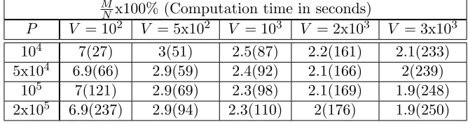
Next we investigated the impact of changes in the values of the parameters P and V on the performance of DeriveRS. All combinations of P = {104,5x104,105,2x105} and V ={102,5x102,103,2x103,3x103}were used to compute the representative set of D1. The computations were performed for= 10−2 and g= 1. The method FLS2 was used for the first level segregation in DeriveRS. The results are shown in Table 1. As expected for an
algorithm of time complexityO(N(log2NP +PV + log2V) +V
Q
P
q=1 R
P
r=1
S(Aqr)), the computation
time was generally observed to increase for an increase in the value ofV orP. It should be noted that our implementation of DeriveRS was based on SMO and henceS(Aqr) =O(A
2 qr).
In some cases the computation time decreased whenP orV increased. This is caused by a
decrease in the value of O(
Q
P
q=1 R
P
r=1
A2qr), which is inferred from the observed decrease of the size of the representative set M (M ≈
Q
P
q=1 R
P
r=1
Aqr). A sharp decrease in M was observed
whenV was increased. The impact of increasingP on the size of the representative set was found to be less drastic. This observation indicates that DeriveAE selects fewer approximate extreme points whenV is larger.
M
Nx100% (Computation time in seconds)
P V = 102 V = 5x10² V = 103 V = 2x10³ V = 3x10³
104 7(27) 3(51) 2.5(87) 2.2(161) 2.1(233)
5x10⁴ 6.9(66) 2.9(59) 2.4(92) 2.1(166) 2(239) 105 7(121) 2.9(69) 2.3(98) 2.1(169) 1.9(248) 2x10⁵ 6.9(237) 2.9(94) 2.3(110) 2(176) 1.9(250)
Table 1: The impact of varyingP and V on the result of DeriveRS
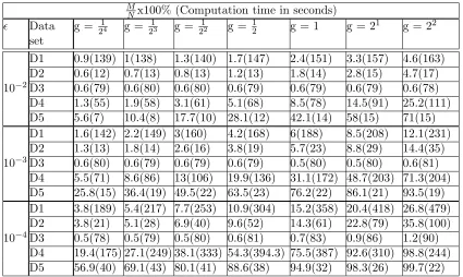
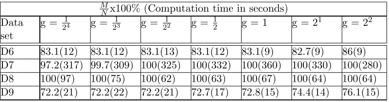
the representative set has to be computed using DeriveRS for all values of kernel hyper-parameter g in the grid. This is because the kernel space varies when the value of g is varied. For all the computations, the input parameters were set as P = 105 and V = 103. The first level segregation in DeriveRS was performed using FLS2. Three values of the tolerance parameterwere investigated, = 10−2,10−3 or 10−4.
The results of the computation for data sets D1 - D5, are shown in the Table 2. The percentage of data vectors in the representative set was found to increase with increasing values of g. This is intuitive, as when g increases the distance between the data vectors in kernel space increases. With increased distances, more data vectorsxi become approximate extreme points. The increase in the number of approximate extreme points with g causes the rising trend of computation time shown in Table 2. For a decrease in the value of , M increases. This is because, for smaller fewer xi would satisfy the condition: optimized p(xi,Ψ) ≤ in CheckPoint(xi,Ψ). This results in the selection of a larger number of approximate extreme points in DeriveAE.
M
Nx100% (Computation time in seconds)
Data
set
g = 214 g = 1
23 g = 1
22 g = 1
2 g = 1 g = 2
1 g = 22
10−2
D1 0.9(139) 1(138) 1.3(140) 1.7(147) 2.4(151) 3.3(157) 4.6(163) D2 0.6(12) 0.7(13) 0.8(13) 1.2(13) 1.8(14) 2.8(15) 4.7(17) D3 0.6(79) 0.6(80) 0.6(80) 0.6(79) 0.6(79) 0.6(79) 0.6(78) D4 1.3(55) 1.9(58) 3.1(61) 5.1(68) 8.5(78) 14.5(91) 25.2(111) D5 5.6(7) 10.4(8) 17.7(10) 28.1(12) 42.1(14) 58(15) 71(15)
10−3
D1 1.6(142) 2.2(149) 3(160) 4.2(168) 6(188) 8.5(208) 12.1(231) D2 1.3(13) 1.8(14) 2.6(16) 3.8(19) 5.7(23) 8.8(29) 14.4(35) D3 0.6(80) 0.6(79) 0.6(79) 0.6(79) 0.5(80) 0.5(80) 0.6(81) D4 5.5(71) 8.6(86) 13(106) 19.9(136) 31.1(172) 48.7(203) 71.3(204) D5 25.8(15) 36.4(19) 49.5(22) 63.5(23) 76.2(22) 86.1(21) 93.5(19)
10−4
D1 3.8(189) 5.4(217) 7.7(253) 10.9(304) 15.2(358) 20.4(418) 26.8(479) D2 3.8(21) 5.1(28) 6.9(40) 9.6(52) 14.3(61) 22.8(79) 35.8(100) D3 0.5(78) 0.5(79) 0.5(80) 0.6(81) 0.7(83) 0.9(86) 1.2(90) D4 19.4(175) 27.1(249) 38.1(333) 54.3(394.3) 75.5(387) 92.6(310) 98.8(244) D5 56.9(40) 69.1(43) 80.1(41) 88.6(38) 94.9(32) 98.3(26) 99.7(22)
Table 2: The percentage of the data vectors in X∗ (given by MNx100) and its computation time for data sets D1-D5
M
Nx100% (Computation time in seconds)
Data set
g = 214 g = 213 g = 212 g = 12 g = 1 g = 21 g = 22
D6 83.1(12) 83.1(12) 83.1(13) 83.1(12) 83.1(9) 82.7(9) 86(9) D7 97.2(317) 99.7(309) 100(325) 100(332) 100(360) 100(330) 100(280) D8 100(97) 100(75) 100(62) 100(63) 100(67) 100(64) 100(64) D9 72.2(21) 72.2(22) 72.2(21) 72.7(17) 72.8(15) 74.4(14) 76.1(15)
Table 3: The percentage of data vectors inX∗and its computation time for data sets D6-D9 with= 10−2
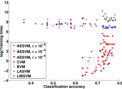
5.3 Comparison of AESVM to SVM Solvers
To judge the accuracy and efficiency of AESVM, its classification performance was compared with the SMO implementation in LIBSVM, ver. 3.1. We chose LIBSVM because it is a state-of-the-art SMO implementation that is routinely used in similar comparison studies. To compare the efficiency of AESVM to other popular approximate SVM solvers we chose CVM, BVM, LASVM, SVMperf, and RfeatSVM. A description of these methods is given in Section 2. We chose these methods because they are widely cited, their software implementations are freely available and other studies (Shalev-Shwartz et al., 2011) have reported fast SVM training using some of these methods. LASVM is also an efficient method for online SVM training. However, since we do not investigate online SVM learning in this paper, we did not test the online SVM training performance of LASVM. We compared AESVM with CVM and BVM even though they are L2-SVM solvers, as they has been reported to be faster alternatives to SVM implementations such as LIBSVM.
The implementation of AESVM and DeriveRS were built upon the LIBSVM implemen-tation. All methods except SVMperfwere allocated a cache of size 600 MB. The parameters for DeriveRS were P = 105 and V = 103, and the first level segregation was performed using FLS2. To reflect a typical SVM training scenario, we performed a grid search with all eighty four combinations of the SVM hyper-parameters C0 = {2−4,2−3, ...,26,27} and g = {2−4,2−3,2−2, ...,21,22}. As mentioned earlier, for data sets D2, D3 and D4, five fold cross-validation was performed. The results of the comparison have been split into sub-sections given below, due to the large number of SVM solvers and data sets used.
5.3.1 Comparison to CVM, BVM, LASVM and LIBSVM
number of support vectors. It can be seen that, AESVM generally gave more accurate results for a fraction of the training time of the other algorithms, and also resulted in less classification time. The training time and classification times of AESVM increased when was reduced. This is expected given the inverse relation of M to shown in Tables 2 and 3. The variation in accuracy with is not very noticeable.
0.4
0.5
0.6
0.7
0.8
−
4
−
2
0
2
4
6
8
10
12
log(Training time)
Classification accuracy
AESVM,
ε
= 10
−2AESVM,
ε
= 10
−3AESVM,
ε
= 10
−4CVM
BVM
LASVM
LIBSVM
Figure 2: Plot of training time against classification accuracy of the SVM algorithms on D2
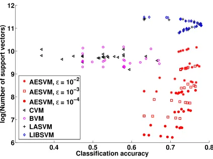
Figures 2 and 3 indicate that AESVM gave better results than the other algorithms for SVM training and classification on D2, in terms of standard metrics. To present a more quantitative and easily interpretable comparison of the algorithms, we define the seven performance metrics given below. These metrics combine the results of all runs of each algorithm into a single value, for each data set. For the first five metrics, we take LIBSVM as a baseline of comparison, as it gives the most accurate solution among the tested methods. Furthermore, an important objective of these experiments is to show the similarity of the results of AESVM and LIBSVM. In the description given below, F can refer to any SVM
0.4
0.5
0.6
0.7
0.8
6
7
8
9
10
11
12
log(Number of support vectors)
Classification accuracy
AESVM,
ε
= 10
−2AESVM,
ε
= 10
−3AESVM,
ε
= 10
−4CVM
BVM
LASVM
LIBSVM
Figure 3: Plot of classification time, represented by the number of support vectors, against classification accuracy of the SVM algorithms on D2
1. Expected training time speedup, ET S: The expected speedup in training time is indi-cated by:
ET S = 1 RS
R
X
r=1 S
X
s=1
T Lrs TFrs
.
Here T Lrs and TFrs are the training times of LIBSVM and F respectively, in the sth
cross-validation fold with the rth set of hyper-parameters of grid search.
2. Overall training time speedup, OT S: It indicates overall training time speedup for the entire grid search with cross-validation, including the time taken to compute the representative set. The total time taken by DeriveRS to compute the representative set for all values of g is represented as TX∗. For methods other than AESVM and
RfeatSVM2 (see Section 5.3.3),TX∗= 0.
OT S=
R
P
r=1 S
P
s=1
T Lrs
R
P
r=1 S
P
s=1
TFrs+TX∗
3. Expected classification time speedup, ECS: The expected speedup in classification time is indicated by:
ECS = 1
RS R X r=1 S X s=1
N Lrs NFrs
.
HereN LrsandNFrs are the number of support vectors in the solution of LIBSVM and Frespectively.
4. Classification time speedup for optimal hyper-parameters,CT S: The speedup in classi-fication time for the optimal hyper-parameters (hyper-parameters that result in max-imum classification accuracy) chosen by grid search is indicated by:
CT S=
max r
S
P
s=1
N Lrs
max r
S
P
s=1
NFrs
.
5. Root mean squared error of classification accuracy, RM SE: The similarity of the solution ofF to LIBSVM, in terms of its classification accuracy, is indicated by:
RM SE = 1
RS R X r=1 S X s=1
(CLrs−CFrs)2
!0.5
.
Here CLrs and CFrs are the classification accuracy of LIBSVM and Frespectively.
6. Maximum classification accuracy: It gives the best classification results of an SVM solver, for the set of SVM hyper-parameters that are tested.
max. acc. =max r 1 S S X s=1
CFrs.
7. Mean and standard deviation of classification accuracies: It indicates the classification performance of an SVM solver, that can be expected for arbitrary hyper-parameter values.
mean acc. = 1 RS R X r=1 S X s=1
CFrs, and std. acc. =
v u u t1 R R X r=1 1 S S X s=1
CFrs−mean acc.
!2
.
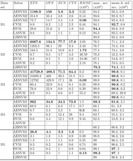
Data set
Solver ET S OT S ECS CT S RM SE
(x102)
max. acc. (x102)
mean & std. acc. (x102)
D1
AESVM1 1188.9 156 5.8 3.3 0.22 94.2 92.4, 0.8
AESVM2 314.8 50.4 3.8 2.6 0.14 93.6 92.3, 0.7
AESVM3 72.7 14.7 2.4 1.8 0.06 93.8 92.4, 0.8
CVM 8.9 6.2 1.2 2.3 0.44 94.1 92.7, 0.8
BVM 28.6 21.6 2 1.9 0.6 94.4 92.6, 0.9
LASVM 0.8 0.8 1.1 1 0.12 94.3 92.5, 0.8
LIBSVM 93.9 92.4, 0.8
D2
AESVM1 6067.6 134.5 77.7 17.8 3.85 76.5 71.1, 3.3
AESVM2 1202.5 86.1 29 9.4 2.43 76.7 72.4, 3.6
AESVM3 164.5 21.8 10.9 6.2 1.73 77.4 73.1, 3.6
CVM 0.7 0.5 4.7 4.3 26.59 70.3 52.2, 0.8
BVM 0.8 0.5 5 5.6 24.06 67.1 54.6, 0.7
LASVM 0.2 0.1 1 1 2.18 78.1 73.5, 0.5
LIBSVM 78.2 74.1, 3.5
D3
AESVM1 41728.8 488.5 71.5 64.4 0.2 99.9 99.8, 0.1
AESVM2 21689.3 468 39.5 51.5 0.1 99.9 99.8, 0.1
AESVM3 12792 429.9 17.1 36 0.09 99.9 99.8, 0.1
CVM 60.4 23.9 0.4 0.1 0.33 99.9 99.8, 0.2
BVM 76.8 22.8 0.6 0.2 0.39 99.9 99.8, 0.2
LASVM 0.9 0.5 0.6 0.7 55.2 99.9 69.3, 29.9
LIBSVM 99.9 99.8, 0.1
D4
AESVM1 962 34.6 24.5 72.8 1.5 68.3 61.6, 3.1
AESVM2 68.8 6.1 6.3 17.1 0.7 68.1 61, 3.3
AESVM3 6.7 2.3 2.3 5 0.3 68.1 60.8, 3.2
CVM 8 6.2 12.4 28 9.4 63.7 55.5, 3.1
BVM 6.6 4.4 12.1 8.9 9.44 62.3 54.9, 3.4
LASVM - - -
-LIBSVM 68.2 60.6, 3.2
D5
AESVM1 26.6 4.1 3.3 1.6 0.5 98.8 96.2, 2.6
AESVM2 3.1 1.8 1.5 0.9 0.39 98.9 96.3, 2.6
AESVM3 1.3 1.1 1.1 0.9 0.25 99 96.4, 2.6
CVM 0.3 0.2 0.8 0.6 0.74 99 96.6, 2.5
BVM 0.5 0.3 1 0.9 0.84 99.1 97, 2
LASVM 0.6 0.5 1 1.1 0.13 99.2 97, 2
LIBSVM 99 96.6, 2.4
Comparing AESVM to CVM, BVM and LASVM, we see that AESVM in general gave the least values of RM SE and the largest values of ET S, OT S, ECS and CT S. In a few cases LASVM gave lowRM SE values. However, in all our experiments LASVM took longer to train than the other algorithms including LIBSVM. We could not complete the evaluation of LASVM for D4 due to its large training time, which was more than 40 hours for some hyper-parameter combinations. The five algorithms under comparison were found to give similar maximum classification accuracies for D1, D3 and D5. For D2 and D4, CVM and BVM gave significantly smaller maximum classification accuracies. Another interesting result is that for D3, the mean and standard deviation of classification accuracy of LASVM was found to be widely different from the other algorithms. For all the tested values of the maximum, mean and standard deviation of the classification accuracies of AESVM were found to be similar.
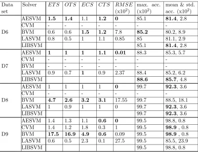
Next we present the results of performance comparison of CVM, BVM, LASVM, AESVM, and LIBSVM on the high-dimensional data sets D6-D9. As described in Section 5.2, De-riveRS was run with only = 10−2 for these data sets. The results of the performance comparison are shown in Table 5. CVM was found to take longer than 40 hours to train on D6, D7 and D8 with some hyper-parameter values and hence we could not complete its evaluation for those data sets. BVM also took longer than 40 hours to train on D7 and it was also not evaluated for D7. AESVM consistently reportedET S,OT S,ECS and CT S values that are larger than 1 unlike the other algorithms, except for D9 where the CT S value for AESVM was 0.6. However it should be noted that the other methods also had sim-ilarly lowCT S values for D9. Similar to the results in Table 4, LASVM and BVM resulted in very largeRM SE values for some data sets. The maximum classification accuracies of all algorithms were similar. On some data sets, BVM and LASVM were observed to give significantly lower mean and higher standard deviation of classification accuracy.
5.3.2 Comparison to SVMperf
SVMperf differs from the other SVM solvers in its ability to compute a solution close to the SVM solution for a given number of support vectors (k). The algorithm complexity depends onkasO(k2) per iteration. We first used a value ofk= 1000 for our experiments,
as it has been reported to give good performance (Joachims and Yu, 2009). SVMperf was tested on data sets D1, D4, D5, D6, D8 and D9, with the Gaussian kernel12 and the same hyper-parameter grid as described earlier. The results of the grid search are presented in Table 6. The results of our experiments on AESVM (with = 10−2) and LIBSVM are repeated in Table 6 for ease of reference. The maximum, mean and standard deviation of classification accuracies are represented as max. acc., mean & std. acc. respectively.
Based on the results obtained fork= 1000, other values ofkwere also tested. For data sets D1, D4 and D5, though SVMperf gave classification accuracies similar to the that of LIBSVM and AESVM, the training times were similar to or higher than the training times of LIBSVM. To test the ability of SVMperf to give fast training, we also tested it withk= 400 for D1, D4 and D5. For the high dimensional data sets (D6, D8 and D9), theRM SE values were significantly higher for SVMperf, while the mean classification accuracy was noticeably lower than AESVM. Considering the possibility that the value ofk= 1000 is insufficient to
Data set
Solver ET S OT S ECS CT S RM SE (x102)
max. acc. (x102)
mean & std. acc. (x102)
D6
AESVM 1.5 1.4 1.1 1.2 0 85.1 81.4, 2.8
CVM - - -
-BVM 0.6 0.6 1.5 1.2 7.8 85.2 80.2, 8.9
LASVM 0.8 0.5 1 1.1 0.85 85 81.1, 2.9
LIBSVM 85.1 81.4, 2.8
D7
AESVM 1 1 1 1.1 0.01 88.3 85.3, 5.7
CVM - - -
-BVM - - -
-LASVM 0.9 0.7 1 0.9 2.37 88.4 85.2, 6.2
LIBSVM 88.6 85.7, 4.8
D8
AESVM 1 1 1 1 0 99.7 92.3, 3.6
CVM - - -
-BVM 4.7 2.6 3.2 3.1 17.55 99.7 88.5, 18.1
LASVM 1 0.9 1 1 0 99.7 92.3, 3.6
LIBSVM 99.7 92.3, 3.6
D9
AESVM 1.4 1.3 1.1 0.6 0 99.5 98.8, 0.8
CVM 1.4 1.2 1.8 0.3 1 99.5 98.9 , 0.8
BVM 17.5 16.9 4.9 0.6 0.09 99.5 98.9 , 0.8
LASVM 0.6 0.5 2.3 0.1 27.5 99.5 85.5, 23.9
LIBSVM 99.5 98.8, 0.8
Table 5: Performance comparison of AESVM (with = 10−2), CVM, BVM, LASVM and LIBSVM on data sets D6-D9
result in an accurate solution for these data sets, we tested D6 and D9 with k= 2000 and D8 withk= 3000. Even though the training time increased significantly with an increase in k, the values ofRM SEand the mean and standard deviation of accuracies did not improve significantly. The training time speedup values of SVMperf are much lower than AESVM for all tested k values for all data sets, except for D8. The maximum accuracies of all the algorithms were similar. Due to the ability of SVMperfto approximatewwith a small set of kvectors, the classification time speedups of SVMperfare significantly higher than AESVM. However, this approximation comes at the cost of increased training time and sometimes results in a loss of accuracy, as illustrated in Table 6.
5.3.3 Comparison to RfeatSVM
Data set
Solver ET S OT S ECS CT S RM SE
(x102)
max. acc. (x102)
mean & std. acc. (x102)
D1
AESVM 1188.9 156 5.8 3.3 0.22 94.2 92.4, 0.8
SVMperf k = 400
6.7 1.6 17 6.6 0.89 93.9 92.7, 0.4
SVMperf k = 1000
3.7 0.9 2.6 2.6 0.74 94 92.7, 0.5
LIBSVM 93.9 92.4, 0.8
D4
AESVM 962 34.6 24.5 72.8 1.5 68.3 61.6, 3.1
SVMperf k = 400
10.2 3.7 467.1 694.3 3.7 68.4 62.9, 2.2
SVMperf k = 1000
3.1 1.2 186.8 277.7 2.14 68.1 61.8, 2.7
LIBSVM 68.2 60.6, 3.2
D5
AESVM 26.6 4.1 3.3 1.6 0.5 98.8 96.2, 2.6
SVMperf k = 400
0.8 0.4 14.6 8.2 2.9 98.8 96.5, 2.4
SVMperf k = 1000
0.2 0.1 5.8 3.3 0.26 99 96.7, 2.4
LIBSVM 99 96.6, 2.4
D6
AESVM 1.5 1.4 1.1 1.2 0 85.1 81.4, 2.8
SVMperf k = 1000
1.1 0.9 20 12.1 9.39 85.2 79.6, 10.7
SVMperf k = 2000
0.3 0.2 10 6 6.5 85.1 80.1, 7.8
LIBSVM 85.1 81.4, 2.8
D8
AESVM 1 1 1 1 0 99.7 92.3, 3.6
SVMperf k = 1000
37.6 23.8 49 9.9 54.2 99.9 55.7, 42.3
SVMperf k = 3000
3.5 1.2 16.3 3.3 51.4 99.8 59.2, 41.6
LIBSVM 99.7 92.3, 3.6
D9
AESVM 1.4 1.3 1.1 0.6 0 99.5 98.8, 0.8
SVMperf k =1000
1.2 0.9 21.3 3 22.6 99.2 86.1, 18.8
SVMperf k =2000
0.4 0.3 10.7 1.5 20.6 99.4 87.3, 17.3
LIBSVM 99.5 98.8, 0.8
Table 6: Performance comparison of SVMperf, AESVM (with= 10−2), and LIBSVM
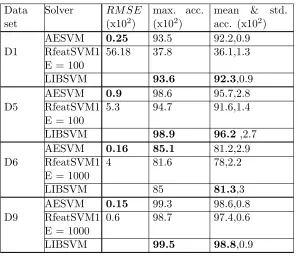
in spite of the availability of faster linear SVM implementations, as it is an exact SVM solver. Hence only the performance metrics related to accuracy were used to compare the performance of AESVM, LIBSVM and RfeatSVM1. The random Fourier features method, described in Algorithm 1 of Rahimi and Recht (2007), was used to project the data sets D1, D5, D6 and D9 into a randomized feature space of dimension E.
Data set
Solver RM SE
(x102)
max. acc. (x102)
mean & std. acc. (x102) D1
AESVM 0.25 93.5 92.2,0.9
RfeatSVM1 E = 100
56.18 37.8 36.1,1.3
LIBSVM 93.6 92.3,0.9
D5
AESVM 0.9 98.6 95.7,2.8
RfeatSVM1 E = 100
5.3 94.7 91.6,1.4
LIBSVM 98.9 96.2 ,2.7
D6
AESVM 0.16 85.1 81.2,2.9
RfeatSVM1 E = 1000
4 81.6 78,2.2
LIBSVM 85 81.3,3
D9
AESVM 0.15 99.3 98.6,0.8
RfeatSVM1 E = 1000
0.6 98.7 97.4,0.6
LIBSVM 99.5 98.8,0.9
Table 7: Performance comparison of RfeatSVM1 (RfeatSVM solved using LIBSVM), AESVM (with = 10−2), and LIBSVM
The results of the accuracy comparison are given in Table 7. We used a smaller hyper-parameter grid of all twenty four combinations of C0 = {2−4,2−2,1,22,24,26} and g = {2−4,2−2,1,22} for our experiments. The results reported in Table 7 for AESVM and LIBSVM were computed for this smaller grid. We selected the number of dimensions (E) of the randomized feature space for D1 and D6 based on Rahimi and Recht (2007). The maximum accuracy for RfeatSVM1 was found to be much less than AESVM and LIBSVM for all data sets. TheRM SE values for RfeatSVM1 were significantly higher than AESVM and mean accuracy noticeably lower for most data sets, especially for D1 and D6.
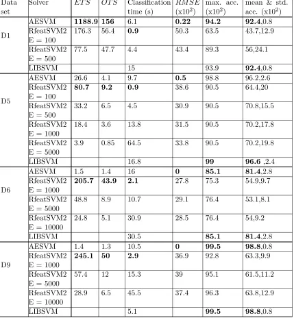
Next we investigated the training and classification time requirements of RfeatSVM by solving it using the fast linear SVM solver LIBLINEAR (Fan et al., 2008), referred to as RfeatSVM2 in the remainder of this paper. The entire hyper-parameter grid used in the previous sections were used in this experiment. The results of the performance comparison of RfeatSVM2, AESVM and LIBSVM are presented in Table 8. Theclassification time
Data set
Solver ET S OT S Classification time (s)
RM SE (x102)
max. acc. (x102)
mean & std. acc. (x102)
D1
AESVM 1188.9 156 6.1 0.22 94.2 92.4,0.8
RfeatSVM2 E = 100
176.3 56.4 0.9 50.3 63.5 43.7,12.9
RfeatSVM2 E = 500
77.5 47.7 4.4 43.4 89.3 56,24.1
LIBSVM 15 93.9 92.4,0.8
D5
AESVM 26.6 4.1 9.7 0.5 98.8 96.2,2.6
RfeatSVM2 E = 100
80.7 9.2 0.9 38.6 90.5 64.4,20
RfeatSVM2 E = 500
33.2 6.5 4.5 30.9 90.5 70.8,15.5
RfeatSVM2 E = 1000
18.4 3.6 13.8 31.5 90.5 70.2,17.8
RfeatSVM2 E = 5000
3.9 0.85 64.5 33.8 90.5 70.2,19.8
LIBSVM 16.8 99 96.6 ,2.4
D6
AESVM 1.5 1.4 16 0 85.1 81.4,2.8
RfeatSVM2 E = 1000
205.7 43.9 2.1 27.8 75.3 54.9,9.7
RfeatSVM2 E = 5000
48.8 8.9 10.7 29.1 76.4 53.1,8.1
RfeatSVM2 E = 10000
24.8 5.1 30.9 28.5 76.4 54,9.2
LIBSVM 30.5 85.1 81.4,2.8
D9
AESVM 1.4 1.3 10.5 0 99.5 98.8,0.8
RfeatSVM2 E = 1000
245.1 50 2.9 36.9 92.8 63.3,9.9
RfeatSVM2 E = 5000
57.4 12 15.3 39 95.1 61.5,11.2
RfeatSVM2 E = 10000
28.9 6.5 45.5 37.4 96.3 63.8,12.9
LIBSVM 5.1 99.5 98.8,0.8
Table 8: Performance comparison of RfeatSVM2 (RfeatSVM solved using LIBLINEAR), AESVM (with = 10−2), and LIBSVM
its optimal hyper-parameters. For RfeatSVM2 the classification time includes the time taken to derive the random Fourier features of the test vectors.
speed-ups than AESVM for small values of E, except for D1 where AESVM was much faster. However, with increasing E the classification time and training time increased to more than AESVM for most data sets. For all data sets, theRM SE, and maximum, mean and standard deviation of accuracy of RfeatSVM2 were significantly worse than AESVM. Increasing the number of dimensions E, resulted in only a slight improvement in the clas-sification performance of RfeatSVM2. An important observation was that the projected data sets were found to be almost 100% dense, which results in large memory requirements for RfeatSVM1 and RfeatSVM2. Even though, technically the value of E can be increased arbitrarily, its value is practically limited by the memory requirements of RfeatSVM.
5.4 Performance with the Polynomial Kernel
To validate our proposal of AESVM as a fast alternative to SVM for all non-linear kernels, we performed a few experiments with the polynomial kernel, k(x1,x2) = (1 +xT1x2)d. The hyper-parameter grid composed of all twelve combinations of C0 = {2−4,2−2,1,22} and d={2,3,4} was used to compute the solutions of AESVM and LIBSVM on the data sets D1, D4 and D6. The results of the computation of the representative set using DeriveRS are shown in Table 9. The parameters for DeriveRS wereP = 105,V = 103 and = 10−2, and the first level segregation was performed using FLS2. The performance comparison of AESVM and LIBSVM with the polynomial kernel is shown in Table 10. Like in the case of the Gaussian kernel, we found that AESVM gave results similar to LIBSVM with the polynomial kernel, while taking shorter training and classification times.
M
Nx100% (Computation time in seconds)
Data set
d = 2 d = 3 d = 4
D1 8(109) 13.2(199) 26(638) D4 20.1(67) 48(260.1) 81.3(1166.4) D6 87.8(11) 84(12.5) 91(13.7)
Table 9: Results of DeriveRS for the polynomial kernel
6. Discussion
Data set
Solver ET S OT S ECS CT S RM SE (x102)
max. acc. (x102)
mean & std. acc. (x102)
D1 AESVM 21.1 6.4 2.7 2.6 0.13 93.9 93.4, 0.4
LIBSVM 94.1 93.5, 0.4
D4 AESVM 7 1.6 2.6 1.9 0.8 64.9 61.2, 2.7
LIBSVM 64.5 60.7, 2.5
D6 AESVM 3.8 5.3 1.1 1.1 0.04 84.6 81, 2.4
LIBSVM 84.6 81, 2.3
Table 10: Performance comparison of AESVM (with = 10−2), and LIBSVM with the polynomial kernel
D1 D2 D3 D4 D5 D6 D7 D8 D9
0 20 40 60 80 100
Mean Accuracy x 10
2
Datasets AESVM, ε= 10−2 CVM
BVM LASVM SVMperf RfeatSVM1 LIBSVM
Figure 4: Plot of mean classification accuracy of all SVM solvers
lack of availability of a software implementation and of published results on L1-SVM with non-linear kernels using their approach, the authors find such a comparison study beyond the scope of this paper.
The theoretical and experimental results presented in this paper demonstrate that the solutions of AESVM and SVM are similar in terms of the resulting classification accuracy.
![Figure 1: Performance of variants of DeriveRS with g = [2−4, 2−3, 2−2, ..., 22], for data setsD1, D2, D4, and D5](https://thumb-us.123doks.com/thumbv2/123dok_us/9805342.1966473/20.612.98.518.337.578/figure-performance-variants-derivers-data-setsd-d-d.webp)