Loss Minimization and Parameter Estimation
with Heavy Tails
Daniel Hsu djhsu@cs.columbia.edu
Department of Computer Science Columbia University
New York, NY 10027, USA
Sivan Sabato sabatos@cs.bgu.ac.il
Department of Computer Science Ben-Gurion University of the Negev Beer-Sheva 8410501, Israel
Editor:David Dunson
Abstract
This work studies applications and generalizations of a simple estimation technique that provides exponential concentration under heavy-tailed distributions, assuming only bounded low-order moments. We show that the technique can be used for approximate minimization of smooth and strongly convex losses, and specifically for least squares linear regression. For instance, our d-dimensional estimator requires just ˜O(dlog(1/δ)) random samples to obtain a constant factor approximation to the optimal least squares loss with probability 1−δ, without requiring the covariates or noise to be bounded or subgaussian. We provide further applications to sparse linear regression and low-rank covariance matrix estimation with similar allowances on the noise and covariate distributions. The core technique is a generalization of the median-of-means estimator to arbitrary metric spaces.
Keywords: Heavy-tailed distributions, unbounded losses, linear regression, least squares
1. Introduction
The minimax principle in statistical estimation prescribes procedures (i.e., estimators) that minimize the worst-case risk over a large class of distributions generating the data. For a given loss function, the risk is the expectation of the loss of the estimator, where the expectation is taken over the data examined by the estimator. For example, for a large class of loss functions including squared loss, the empirical mean estimator minimizes the worst-case risk over the class of Gaussian distributions with known variance (Wolfowitz, 1950). In fact, Gaussian distributions with the specified variance are essentially the worst-case family of distributions for squared loss, at least up to constants (see,e.g., Catoni, 2012, Proposition 6.1).
where only very low order moments may be finite. For example, the Pareto distributions with shape parameter α > 0 are unbounded and have finite moments only up to orders
< α; these distributions are commonly associated with the modeling of extreme events that
manifest in data. Bounds on the expected behavior of an estimator are insufficient in these cases, since the high-probability guarantees that may be derived from such bounds (say, using Markov’s inequality) are rather weak. For example, if the risk (i.e., expected loss) of an estimator is bounded by , then all that we may derive from Markov’s inequality is that the loss is no more than /δ with probability at least 1−δ. For small values of
δ ∈ (0,1), the guarantee is not very reassuring, but it may be all one can hope for in these extreme scenarios—see Remark 7 in Section 3.1 for an example where this is tight. Much of the work in statistical learning theory is also primarily concerned with such high probability guarantees, but the bulk of the work makes either boundedness or subgaussian tail assumptions that severely limit the applicability of the results even in settings as simple as linear regression (see, e.g., Srebro et al., 2010; Shamir, 2014).
Recently, it has been shown that it is possible to improve on methods which are optimal for expected behavior but suboptimal when high-probability deviations are concerned (Au-dibert and Catoni, 2011; Catoni, 2012; Brownlees et al., 2014). These improvements, which are important when dealing with heavy-tailed distributions, suggest that new techniques (e.g., beyond empirical risk minimization) may be able to remove the reliance on bound-edness or control of high-order moments. Bubeck et al. (2013) show how a more robust mean estimator can be used for solving the stochastic multi-armed bandit problem under heavy-tailed distributions.
This work applies and generalizes a technique for controlling large deviations from the expected behavior with high probability, assuming only bounded low-order moments such as variances. We show that the technique is applicable to minimization of smooth and strongly convex losses, and derive specific loss bounds for least squares linear regression, which match existing rates, but without requiring the noise or covariates to be bounded or subgaussian. This contrasts with several recent works (Srebro et al., 2010; Hsu et al., 2014; Shamir, 2014) concerned with (possibly regularized) empirical risk minimizers that require such assumptions. It is notable that in finite dimensions, our result implies that a constant factor approximation to the optimal loss can be achieved with a sample size that is independent of the size of the optimal loss. This improves over the recent work of Mahdavi and Jin (2013), which has a logarithmic dependence on the optimal loss, as well as a suboptimal dependence on specific problem parameters (namely condition numbers). We also provide a new generalization of the basic technique for general metric spaces, which we apply to least squares linear regression with heavy tail covariate and noise distributions, yielding an improvement over the computationally expensive procedure of Audibert and Catoni (2011).
although our aim is expressly different in that our aim is good performance on the same probability distribution generating the data, rather than an uncontaminated or otherwise better behaved distribution. Our new technique can be cast as a simple selection problem in general metric spaces that generalizes the scalar median.
We demonstrate the versatility of our technique by giving further examples in sparse linear regression (Tibshirani, 1996) under heavy-tailed noise and low-rank covariance co-variance matrix approximation (Koltchinskii et al., 2011) under heavy-tailed covariate dis-tributions. We also show that for prediction problems where there may not be a reasonable metric on the predictors, one can achieve similar high-probability guarantees by using me-dian aggregation in the output space.
The initial version of this article (Hsu and Sabato, 2013, 2014) appeared concurrently with the simultaneous and independent work of Minsker (2013), which develops a different generalization of the median-of-means estimator for Banach and Hilbert spaces. We pro-vide a new analysis and comparison of this technique to ours in Section 7. We have also since become aware of the earlier work by Lerasle and Oliveira (2011), which applies the median-of-means technique to empirical risks in various settings much like the way we do in Algorithm 3, although our metric formulation is more general. Finally, the recent work of Brownlees et al. (2014) vastly generalizes the techniques of Catoni (2012) to apply to much more general settings, although they retain some of the same deficiencies (such as the need to know the noise variance for the optimal bound for least squares regression), and hence their results are not directly comparable to ours.
2. Overview of Main Results
This section gives an overview of the main results.
2.1 Preliminaries
Let [n] := {1,2, . . . , n} for any natural number n ∈ N. Let 1{P} take value 1 if the predicate P is true, and 0 otherwise. Assume an example space Z, and a distribution D over the space. Further assume a space of predictors or estimatorsX. We consider learning or estimation algorithms that accept as input an i.i.d. sample of size ndrawn from D and a confidence parameter δ ∈ (0,1), and return an estimator (or predictor) ˆw ∈ X. For a (pseudo) metric ρ onX, let Bρ(w0, r) := {w∈X:ρ(w0,w)≤r}denote the ball of radius
r around w0.
We assume a loss function `:Z ×X→R+that assigns a non-negative number to a pair of an example from Z and a predictor fromX, and consider the task of finding a predictor that has a small loss in expectation over the distribution of data points, based on an input sample ofnexamples drawn independently fromD. The expected loss of a predictorw on the distribution is denoted L(w) = EZ∼D(`(Z,w)). Let L? := infwL(w). Our goal is to
find ˆwsuch that L( ˆw) is close to L?.
sub-logarithmically on 1/δ, which is the dependence achieved when the distribution of the excess loss has exponentially decreasing tails. Note that we assume that the value ofδ is provided as input to the estimation algorithm, and only demand the probabilistic guarantee for this given value of δ. Therefore, strictly speaking, the excess loss need not exhibit exponential concentration. Nevertheless, in this article, we shall say that an estimation algorithm achieves exponential concentration whenever it guarantees, on inputδ, an excess loss that grows only as log(1/δ).
2.2 Robust Distance Approximation
Consider an estimation problem, where the goal is to estimate an unknown parameter of the distribution, using a random i.i.d. sample from that distribution. We show throughout this work that for many estimation problems, if the sample is split into non-overlapping subsamples, and estimators are obtained independently from each subsample, then with high probability, this generates a set of estimators such that some fraction of them are close, under a meaningful metric, to the true, unknown value of the estimated parameter. Importantly, this can be guaranteed in many cases even under under heavy-tailed distributions.
Having obtained a set of estimators, a fraction of which are close to the estimated parameter, the goal is now to find a single good estimator based on this set. This goal is captured by the following general problem, which we termRobust Distance Approximation. A Robust Distance Approximation procedure is given a set of points in a metric space and returns a single point from the space. This single point should satisfy the following condition: If there is an element in the metric space that a certain fraction of the points in the set are close to, then the output point should also be close to the same element. Formally, let (X, ρ) be a metric space. LetW ⊆Xbe a (multi)set of size k and let w? be
a distinguished element inX. For α ∈(0,12) and w∈X, denote by ∆W(w, α) the minimal
number r such that |{v ∈ W |ρ(w, v) ≤ r}|> k(12 +α). We often omit the subscript W
and write simply ∆ when W is known. We define the following problem:
Definition 1 (Robust Distance Approximation) Fix α ∈(0,12). Given W and (X, ρ)
as input, return y∈X such thatρ(y, w?)≤Cα·∆W(w?, α), for some constantCα≥0. Cα
is the approximation factorof the procedure.
In some cases, learning with heavy-tailed distributions requires using a metric that de-pends on the distribution. Then, the Robust Distance Estimation procedure has access only to noisy measurements of distances in the metric space, and is required to succeed with high probability. In Section 3 we formalize these notions, and provide simple implementations of Robust Distance Approximation for general metric spaces, with and without direct access to the metric. For the case of direct access to the metric our formulation is similar to that of Nemirovsky and Yudin (1983).
2.3 Convex Loss Minimization
results to the relevant sections. Detailed discussion of related work for each application is also provided in the appropriate sections.
First, we consider smooth and convex losses. We assume that the parameter space Xis a Banach space with a normk · k and a dual norm k · k∗. We prove the following result:1 Theorem 2 There exists an algorithm that accepts as input an i.i.d. sample of sizendrawn fromDand a confidence parameterδ ∈(0,1), and returnswˆ ∈X, such that if the following conditions hold:
• the dual normk · k∗ is γ-smooth;
• there exists α > 0 and sample size nα such that, with probability at least 1/2, the
empirical lossw7→Lˆ(w)isα-strongly convex with respect tok · kwhenever the sample is of size at leastnα;
• n≥Clog(1/δ)·nα for some universal constant C >0;
• w7→`(z,w) is β-smooth with respect to k · k for all z∈ Z;
• w7→L(w) is β¯-smooth with respect to k · k;
then with probability at least 1−δ, for another universal constant C0 >0,
L( ˆw)≤
1 +C
0ββγ¯ dlog(1/δ)e
nα2
L?.
This gives a constant approximation of the optimal loss with a number of samples that does not depend on the value of the optimal loss. The full results for smooth convex losses are provided in Section 4. Theorem 2 is stated in full as Corollary 16, and we further provide a result with more relaxed smoothness requirements. As apparent in the result, the only requirements on the distribution are those that are implied by the strong convexity and smoothness parameters. This allows support for fairly general heavy-tailed distributions, as we show below.
2.4 Least Squares Linear Regression
A concrete application of our analysis of smooth convex losses is linear regression. In linear regression,X is a Hilbert space with an inner producth·,·iX, and it is both the data space
and the parameter space. The loss`≡`sqis the squared loss
`sq((x, y),w) := 1 2(x
>
w−y)2. Lsq and Lsq? are defined similarly to Land L?.
Unlike standard high-probability bounds for regression, we give bounds that make no assumption on the range or the tails of the distribution of the response variables, other than a trivial requirement that the optimal squared loss be finite. The assumptions on the distribution of the covariates are also minimal.
Let Σ be the second-moment operator a 7→ E(XhX,aiX), where X is a random data point from the marginal distribution ofDonX. For a finite-dimensionalX,Σ is simply the (uncentered) covariance matrixE[XX>]. First, consider the finite-dimensional case, where X=Rd, and assumeΣ is not singular. Let k · k2 denote the Euclidean norm in Rd. Under only bounded 4 +moments of the marginal on X(a condition that we specify in full detail in Section 5), we show the following guarantee.
Theorem 3 Assume the marginal of X has bounded 4 + moments. There is a constant
C >0and an algorithm that accepts as input a sample of sizenand a confidence parameter
δ∈(0,1), and returns wˆ ∈X, such that if n≥Cdlog(1/δ), with probability at least 1−δ,
Lsq( ˆw)≤Lsq? +O E(kΣ
−1/2X(X>
w?−Y)k22) log(1/δ)
n
!
.
This theorem is stated in full as Theorem 19 in Section 5. Under standard finite fourth-moment conditions, this result translates to the bound
Lsq( ˆw)≤
1 +O
dlog(1/δ)
n
Lsq? ,
with probability≥1−δ. These results improve over recent results by Audibert and Catoni (2011), Catoni (2012), and Mahdavi and Jin (2013). We provide a full comparison to related work in Section 5.
Theorem 3 can be specialized for specific cases of interest. For instance, suppose X is bounded and well-conditioned in the sense that there exists R < ∞ such that Pr[X>
Σ−1X ≤ R2] = 1, but Y may still be heavy-tailed. Under this assumption we have the following result.
Theorem 4 Assume Σ is not singular. There exists an algorithm that accepts as input a sample of size n and a confidence parameter δ ∈(0,1), and returns wˆ ∈X, such that with probability at least 1−δ, for n≥O(R2log(R) log(e/δ)),
Lsq( ˆw)≤
1 +O
R2log(1/δ)
n
Lsq? .
This theorem is stated in full as Theorem 20 in Section 5. Note that
E(X>Σ−1X) =Etr(X>Σ−1X) = tr(Id) =d,
2.5 Other Applications, Comparisons, and Extensions
The general method studied here allows handling heavy tails in other applications as well. We give two examples in Section 6. First, we consider parameter estimation using L1 -regularized linear least squares regression (Lasso) under random subgaussian design. We show that using the above approach, parameter estimation bounds can be guaranteed for general bounded variance noise, including heavy-tailed noise. This contrasts with standard results that assume sub-Gaussian noise. Second, we show that low-rank covariance matrix approximation can be obtained for heavy-tailed distributions, under a bounded 4 + mo-ment assumption. These two applications have been analyzed also in the independent and simultaneous work of Minsker (2013).
All the results above are provided using a specific solution to the Robust Distance Approximation problem, which is easy to implement for any metric space. For the case of a fully known metric, in a Banach or a Hilbert space, Minsker (2013) proposed a different solution, which is based on the geometric median. In Section 7, we provide a detailed comparison of the approximation factor achieved by each approach, as well as some general lower bounds. Several interesting open questions remain regarding this general problem.
Lastly, in Section 8, we give a short proof to the intuitive fact that in some prediction problem, one can replace Robust Distance Approximation with taking the median of the predictions of the input estimators. This gives a possible improper-learning algorithm for relevant learning settings.
All of the techniques we have developed in this work are simple enough to implement and empirically evaluate, and indeed in some simulated experiments, we have verified the improvements over standard methods such as the empirical mean when the data follow heavy-tailed distributions. However, at present, the relatively large constant factors in our bounds are real enough to restrict the empirical improvements only to settings where very high confidence (i.e., small values of δ) is required. By contrast, with an appropriately determined noise variance, the techniques of Catoni (2012) and Brownlees et al. (2014) may yield improvements more readily. Nevertheless, since our techniques are more general in some respects, it is worth investigating whether they can be made more practical (e.g., with greater sample reuse or overlapping groups), and we plan to do this in future work.
3. The Core Techniques
In this section we present the core technique used for achieving exponential concentration. We first demonstrate the underlying principle via the median-of-means estimator, and then explain the generalization to arbitrary metric spaces. Finally, we show a new generalization that supports noisy feature measurements.
3.1 Warm-up: Median-of-Means Estimator
Algorithm 1 Median-of-means estimator
input SampleS ⊂Rof size n, number of groupsk∈Nsuch that k≤n/4. output Population mean estimate ˆµ∈R.
1: Randomly partitionS into ksubsets S1, S2, . . . , Sk, each of size at least bn/kc.
2: For eachi∈[k], letµi ∈R be the sample mean ofSi.
3: Return ˆµ:= median{µ1, µ2, . . . , µk}.
of each group. Note that the possible non-uniqueness of the median does not affect the result; the arguments below apply to any one of them. The input parameter k should be thought of as a constant determined by the desired confidence level (i.e.,k= Θ(log(1/δ)) for confidence δ ∈ (0,1)). It is well known that the median-of-means achieves estimation with exponential concentration. The following proposition gives a simple statement and proof. The constant 6 in the statement (see Eq. (1) below) is lower the constant in the analysis of Lerasle and Oliveira (2011, Proposition 1), which is 2√6e≈8.08, but we require a larger value ofn. By requiring an even largern, the constant in the statement below can approach 3√3.
Proposition 5 Let xbe a random variable with meanµand variance σ2<∞, and letS be a set ofnindependent copies ofx. Assumek≤n/2. With probability at least1−e−k/4.5, the estimate µˆ returned by Algorithm 1 on input (S, k) satisfies|ˆµ−µ| ≤σp8k/n. Therefore, if k= 4.5dlog(1/δ)e and n≥18dlog(1/δ)e, then with probability at least1−δ,
|ˆµ−µ| ≤6σ r
dlog(1/δ)e
n . (1)
Proof First, assumek dividesn. Pick any i∈[k], and observe that Si is an i.i.d. sample
of sizen/k. Therefore, by Chebyshev’s inequality, Pr[|µi−µ| ≤p6σ2k/n]≥5/6. For each
i∈[k], letbi :=1{|µi−µ| ≤p
6σ2k/n}. Note that thebiare independent indicator random variables, each withE(bi)≥5/6. By Hoeffding’s inequality, Pr[Pki=1bi> k/2]≥1−e−k/4.5.
In the event that Pki=1bi > k/2, at least half of the µi are within p
6σ2k/n of µ, which means that the same holds for the median of theµi. Ifkdoes not dividenthen the analysis can be carried out by substitutingnwithbn/kck≥n−k≥ 3
4n, which scales the guarantee by a factor of p4/3.
Using the terminology of Robust Distance Approximation with the metricρ(x, y) =|x−
y|, the proof shows that with high probability over the choice ofW, ∆W(µ,0)≤ p
12σ2k/n. The result then immediately follows because on the space (R, ρ), the median is a Robust Distance Approximation procedure with C0 = 1.
Remark 6 (Catoni’s M-estimator) Catoni (2012) proposes a mean estimator µˆ that satisfies|ˆµ−µ|=O(σplog(1/δ)/n) with probability at least1−δ. Remarkably, the leading constant in the bound is asymptotically optimal: it approaches √2 as n → ∞. However, the estimator takes both δ and σ as inputs. Catoni also presents an estimator that takes only σ as an input; this estimator guarantees a O(σlog(1/δ)/√n) bound for all values of
Remark 7 (Empirical mean) Catoni (2012) shows that the empirical mean cannot pro-vide a qualitatively similar guarantee. Specifically, for anyσ > 0 and δ∈(0,1/(2e)), there is a distribution with mean zero and varianceσ2 such that the empirical averageµˆemp of n i.i.d. draws satisfies
Pr
|ˆµemp| ≥
σ
√ 2nδ
1−2eδ
n
n−21
≥2δ. (2)
Therefore the deviation of the empirical mean necessarily scales with 1/√δ rather than
p
log(1/δ) (with probability Ω(δ)).
3.2 Generalization to Arbitrary Metric Spaces
We now consider a simple generalization of the median-of-means estimator for arbitrary metric spaces, first mentioned in Nemirovsky and Yudin (1983). Let X be the parameter (solution) space,w? ∈Xbe a distinguished point inX(the target solution), andρa metric on X(in fact, a pseudometric suffices).
The first abstraction captures the generation of candidate solutions obtained from inde-pendent subsamples. We assume there is an oracle APPROXρ,εwhich satisfies the following
assumptions.
Assumption 1 A query to APPROXρ,ε returns a random w∈Xsuch that Prhρ(w?,w)≤ε
i
≥2/3.
Note that the 2/3 could be replaced by another constant larger than half; we have not optimized the constants. The second assumption regards statistical independence. For an integerk, let w1, . . . ,wk be responses tok separate queries to APPROXρ,ε.
Assumption 2 w1, . . . ,wk are statistically independent.
The proposed procedure, given in Algorithm 2, generateskcandidate solutions by query-ing APPROXρ,ε ktimes, and then selecting a single candidate using a generalization of the
median. Specifically, for each i ∈[k], the smallest ball centered atwi that contains more
than half of{w1,w2, . . . ,wk}is determined; thewi with the smallest such ball is returned.
If there are multiple such wi with the smallest radius ball, any one of them may be
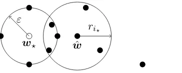
se-lected. This selection method is a Robust Distance Approximation procedure. The proof is given below and illustrated in Figure 1. Nemirovsky and Yudin (1983) proposed a similar technique, however their formulation relies on knowledge of ε.
Proposition 8 Let ri := min{r ≥ 0 : |Bρ(wi, r)∩W| > k/2}. Selecting wi? such that
i?= argminiri is a Robust Distance Approximation procedure withC0 = 3.
Proof Assume that ∆(w?,0)≤ε. Then|Bρ(w?, ε)∩W|> k/2. For anyv∈Bρ(w?, ε)∩W,
by the triangle inequality, |Bρ(v,2ε) ∩W| > k/2. This implies that ri? ≤ 2ε, and so
|Bρ(wi?,2ε)∩W|> k/2. By the pigeonhole principle,Bρ(w?, ε)∩Bρ(wi?,2ε)6=∅.
w? ε
ˆ w
ri?
Figure 1: The argument in the proof of Proposition 8, illustrated on the Euclidean plane. If more than half of thewi (depicted by full circles) are withinεof w? (the empty
circle), then the selectedwi? is withinε+ri? ≤3εofw?.
Algorithm 2 Robust approximation
input Number of candidates k, query access to APPROXρ,ε.
output Approximate solution ˆw∈X.
1: Query APPROXρ,ε ktimes. Letw1, . . . ,wk be the responses to the queries; set W :=
{w1,w2, . . . ,wk}.
2: For eachi∈[k], letri:= min{r≥0 :|Bρ(wi, r)∩W|> k/2}; set i? := arg mini∈[k]ri.
3: Return ˆw:=wi?.
Again, the number of candidateskdetermines the resulting confidence level. The follow-ing theorem provides a guarantee for Algorithm 2. We note that the resultfollow-ing constants here might not be optimal in specific applications, since they depend on the arbitrary constant in Assumption 1.
Proposition 9 Suppose that Assumption 1 and Assumption 2 hold. Then, with probability at least 1−e−k/18, Algorithm 2 returns wˆ ∈
Xsatisfying ρ(w?,w)ˆ ≤3ε.
Proof For each i ∈ [k], let bi := 1{ρ(w?,wi)≤ε}. Note that the bi are independent
indicator random variables, each withE(bi)≥2/3. By Hoeffding’s inequality, Pr[Pki=1bi> k/2]≥1−e−k/18. In the event thatPki=1bi > k/2, more than half of thewi are contained
in the ball of radiusεaround w?, that is ∆W(w?,0)≤ε. The result follows from
Proposi-tion 8.
3.3 Random Distance Measurements
In some problems, the most appropriate metric on X in which to measure accuracy is not directly computable. For instance, the metric may depend on population quantities which can only be estimated; moreover, the estimates may only be relatively accurate with some constant probability. For instance, this is the case when the metric depends on the population covariance matrix, a situation we consider in Section 5.2.3.
To capture such cases, we assume access to a metric estimation oracle as follows. Let
w1, . . . ,wkbe responses tokqueries to APPROXρ,. The metric estimation oracle, denoted
as an estimate ofρ(v,wj). This estimate is required to be weakly accurate, as captured by
the following definition of the random variables Zj. Let f1, . . . , fk be responses to queries to DIST1ρ, . . . ,DISTkρ, respectively. For j∈[k], define
Zj :=1{∀v∈X, (1/2)ρ(v,wj)≤fj(v)≤2ρ(v,wj)}.
Zj = 1 indicates that fj provides a sufficiently accurate estimate of the distances fromwj.
Note thatfj need not correspond to a metric. We assume the following.
Assumption 3 For any j∈[k], Pr[Zj = 1]≥8/9.
We further require the following independence assumption.
Assumption 4 The random variables Z1, . . . , Zk are statistically independent.
Note that there is no assumption on the statistical relationship between Z1, . . . , Zk and
w1, . . . ,wk.
Algorithm 3 is a variant of Algorithm 2 that simply replaces computation ofρ-distances with computations using the functions returned by querying the DISTjρ’s. The resulting selection procedure is, with high probability, a Robust Distance Approximation.
Lemma 10 Consider a run of Algorithm 3, with output wˆ. Let Z1, . . . , Zk as defined above, and suppose that Assumption 3 and Assumption 4 hold. Then, with probability at least 1−e−k/648,
ρ( ˆw,w?)≤9·∆W(w?,
5 36), where W ={w1, . . . ,wk}.
Proof By Assumptions 3 and 4, and by Hoeffding’s inequality,
Pr
k X
j=1
Zj >
31 36k
≥1−e
−k/648 (3)
Assume this event holds, and denote ε= ∆W(w?,365). We have|B(w?, ε)∩W| ≥ 2336k.
Let i∈[k] such that wi ∈Bρ(w?, ε). Then, for any j ∈ [k] such that wj ∈Bρ(w?, ε),
by the triangle inequality ρ(wi,wj) ≤2ε. There are at least 2336k such indices j, therefore
for more thank/2 of the indices j, we have
ρ(wi,wj)≤2εandZj = 1.
For j such that this holds, by the definition of Zj, fj(wi) ≤ 4ε. It follows that ri :=
median{fj(wi)|j∈[k]} ≤4.
Now, let i ∈ [k] such that wi ∈/ B(w?,9). Then, for any j ∈ [k] such that wj ∈ Bρ(w?, ε), by the triangle inequality ρ(wi,wj) ≥ ρ(w?,wi)−ρ(w?,wj) >8ε. As above,
for more thank/2 of the indices j,
ρ(wi,wj)>8εandZj = 1.
For j such that this holds, by the definition of Zj, fj(wi) > 4ε. It follows that ri :=
median{fj(wi)|j∈[k]}>4.
Algorithm 3 Robust approximation with random distances
input Number of candidates k, query access to APPROXρ,ε, query access to DISTρ.
output Approximate solution ˆw∈X.
1: Query APPROXρ,ε ktimes. Letw1, . . . ,wk be the responses to the queries; set W :=
{w1,w2, . . . ,wk}.
2: Fori∈[k], let fi be the response of DISTjρ, and set ri := median{fj(wi) :j∈[k]}; set i? := arg mini∈[k]ri.
3: Return ˆw:=wi?.
1. ri ≤4εfor all wi ∈W ∩Bρ(w?, ε), and
2. ri >4εfor all wi ∈W \Bρ(w?,9ε).
In this event the wi∈W with the smallestri satisfies wi∈Bρ(w?,9ε).
The properties of the approximation procedure and of APPROXρ,are combined to give
a guarantee for Algorithm 3.
Theorem 11 Suppose that Assumptions 1,2,3,4 all hold. With probability at least1−2e−k/648, Algorithm 3 returnswˆ ∈Xsatisfying ρ(w?,w)ˆ ≤9ε.
Proof For each i∈ [k], let bi := 1{ρ(w?,wi)≤ε}. By Assumptions 1 and 2, the bi are
independent indicator random variables, each with E(bi)≥2/3. By Hoeffding’s inequality,
Pr[Pki=1bi > 2336k]≥1−e−k/648. The result follows from Lemma 10 and a union bound. In the following sections we show several applications of these general techniques.
4. Minimizing Strongly Convex Losses
In this section we apply the core techniques to the problem of approximately minimizing strongly convex losses, which includes least squares linear regression as a special case.
4.1 Preliminaries
Suppose (X,k · k) is a Banach space, with the metric ρ induced by the norm k · k. We sometimes denote the metric by k · k as well. Denote by k · k∗ the dual norm, so kyk∗ =
sup{hy,xi:x∈X,kxk ≤1}fory∈X∗.
The derivative of a differentiable function f:X → R at x ∈ X in direction u ∈ X is denoted by h∇f(x),ui. We sayf is α-strongly convex with respect tok · k if
f(x)≥f(x0) +h∇f(x0),x−x0i+α
2kx−x
0k2
for all x,x0∈X; it isβ-smooth with respect to k · kif for all x,x0 ∈X
f(x)≤f(x0) +h∇f(x0),x−x0i+β
2kx−x
We say k · k is γ-smooth if x7→ 1 2kxk
2 is γ-smooth with respect to k · k. We define n
α to
be the smallest sample size such that the following holds: With probability≥5/6 over the choice of an i.i.d. sample T of size |T| ≥nα fromD, for allw∈X,
LT(w)≥LT(w?) +h∇LT(w?),w−w?i+
α
2kw−w?k
2. (4)
In other words, the sampleT induces a lossLT which isα-strongly convex aroundw?.2 We
assume thatnα<∞for someα >0.
We use the following facts in our analysis.
Proposition 12 (Srebro et al., 2010) If a non-negative functionf:X→R+isβ-smooth with respect to k · k, then k∇f(x)k2
∗ ≤4βf(x) for allx∈X.
Proposition 13 (Juditsky and Nemirovski, 2008) LetX1,X2, . . . ,Xnbe independent
copies of a zero-mean random vectorX, and letk · kbeγ-smooth. ThenEkn−1Pni=1Xik2 ≤
(γ/n)EkXk2.
Recall that Z is a data space, and D is a distribution over Z. Let Z be a Z-valued random variable with distributionD. Let`:Z ×X→R+ be a non-negative loss function, and for w∈X, let L(w) :=E(`(Z,w)) be the expected loss. Also define the empirical loss with respect to a sampleT fromZ,LT(w) :=|T|−1Pz∈T`(z,w). To simplify the discussion
throughout, we assume`is differentiable, which is anyway our primary case of interest. We assume that L has a unique minimizer w? := arg minw∈XL(w).3 Let L? := minwL(w).
Setw? such thatL? =L(w?).
4.2 Subsampled Empirical Loss Minimization
To use Algorithm 2, we implement APPROXk·k,ε based on loss minimization over
subsam-ples, as follows: Given a sampleS ⊆ Z, randomly partition S intok groups S1, S2, . . . , Sk,
each of size at leastb|S|/kc, and let the response to thei-th query to APPROXk·k,ε be the
loss minimizer on Si,i.e., wi = arg minw∈XLSi(w). We call this implementation
subsam-pled empirical loss minimization. Clearly, if S is an i.i.d. sample from D, then w1, . . . ,wk
are statistically independent, and so Assumption 2 holds. Thus, to apply Proposition 9, it is left to show that Assumption 1 holds as well.4
The following lemma proves that Assumption 1 holds under these assumptions with
ε:=
r
32γkEk∇`(Z,w?)k2∗
nα2 . (5)
Lemma 14 Letεbe as defined in Eq. (5). Assume k≤n/4, and thatS is an i.i.d. sample fromDof size nsuch that bn/kc ≥nα. Then subsampled empirical loss minimization using
the sample S is a correct implementation of APPROXk·k,ε for up to k queries.
2. Technically, we only need the sample size to guarantee Eq. (4) for allw∈Bk·k(w?, r) for somer >0. 3. This holds, for instance, ifL is strongly convex.
4. An approach akin to the bootstrap technique (Efron, 1979) could also seem natural here: In this approach, S1, . . . , Skwould be generated by randomly sub-sampling fromS, with possible overlap between the
Proof LetT =bn/kc. Sincen≥4k, we havebn/kck≥n−k≥ 3
4n, therefore 1/T ≤ 4k
3n. It
is clear thatw1,w2, . . . ,wk are independent by the assumption. Fix somei∈[k]. Observe
that∇L(w?) =E(∇`(Z,w?)) = 0, and therefore by Proposition 13:
Ek∇LSi(w?)k 2
∗ ≤(γ/T)Ek∇`(Z,w?)k2∗≤
4γk
3n Ek∇`(Z,w?)k
2
∗.
By Markov’s inequality,
Pr
k∇LSi(w?)k 2
∗ ≤
8γk
n E(k∇`(Z,w?)k
2
∗)
≥ 5 6.
Moreover, the assumption that bn/kc ≥ nα implies that with probability at least
5/6, Eq. (4) holds for T = Si. By a union bound, both of these events hold simulta-neously with probability at least 2/3. In the intersection of these events, letting wi :=
arg minw∈XLSi(w),
(α/2)kwi−w?k2 ≤ −h∇LSi(w?),wi−w?i+LSi(wi)−LSi(w?) ≤ k∇LSi(w?)k∗kwi−w?k,
where the last inequality follows from the definition of the dual norm, and the optimality of wi on LSi. Rearranging and combining with the above probability inequality implies
Prhkwi−w?k ≤ε i
≥ 2 3
as required.
Combining Lemma 14 and Proposition 9 gives the following theorem.
Theorem 15 Letnα be as defined in Section 4.1, and assume thatk · k∗ isγ-smooth. Also,
assume k:= 18dlog(1/δ)e, n≥72dlog(1/δ)e, and that S is an i.i.d. sample from D of size
n such that bn/kc ≥nα. Finally, assume Algorithm 3 uses the subsampled empirical loss
minimization to implement APPROXk·k,ε, where ε is as in Eq. (5). Then with probability
at least 1−δ, the parameter wˆ returned by Algorithm 2 satisfies
kwˆ −w?k ≤72 r
γdlog(1/δ)eEk∇`(Z,w?)k2∗
nα2 .
We give an easy corollary of Theorem 15 for the case where `is smooth. This is the full version of Theorem 2.
Corollary 16 Assume the same conditions as Theorem 15, and also that: • w7→`(z,w) is β-smooth with respect to k · k for all z∈ Z;
• w7→L(w) is β¯-smooth with respect to k · k.
Then with probability at least 1−δ,
L( ˆw)≤
1 +10368β ¯
βγdlog(1/δ)e
nα2
Proof This follows from Theorem 15 by first concluding thatE[k∇`(Z,w?)k2∗]≤4βL(w?),
using the β-strong smoothness assumption on ` and Proposition 12, and then noting that
L( ˆw)−L(w?) ≤
¯
β
2kwˆ −w?k2, due to the strong smoothness of L and the optimality of
L(w?).
Corollary 16 implies that for smooth losses, Algorithm 2 provides a constant factor ap-proximation to the optimal loss with a sample size max{nα, γββ/α¯ 2} ·O(log(1/δ)) (with probability at least 1−δ). In subsequent sections, we exemplify cases where the two argu-ments of the max are roughly of the same order, and thus imply a sample size requirement ofO(γββ/α¯ 2log(1/δ)). Note that there is no dependence on the optimal lossL(w?) in the
sample size, and the algorithm has no parameters besides k=O(log(1/δ)).
We can also obtain a variant of Theorem 15 based on Algorithm 3 and Theorem 11, in which we assume that there exists some sample size nk,DISTk·k that allows DISTk·k to
be correctly implemented using an i.i.d. sample of size at least nk,DISTk·k. Under such an
assumption, essentially the same guarantee as in Theorem 15 can be afforded to Algorithm 3 using the subsampled empirical loss minimization to implement APPROXk·k,ε (for ε as in
Eq. (5)) and the assumed implementation of DISTk·k. Note that since Theorem 11 does not
require APPROXk·k,εand DISTk·kto be statistically independent, both can be implemented
using the same sample.
Theorem 17 Letnαbe as defined in Section 4.1,nk,DISTk·k be as defined above, and assume
that k · k∗ is γ-smooth. Also, assume k := 648dlog(2/δ)e, S is an i.i.d. sample from D of size n such that n ≥ max{4k, nk,DISTk·k}, and bn/kc ≥ nα. Further, assume Algorithm 3
implementsAPPROXk·k,ε using S with subsampled empirical loss minimization, where εis
as in Eq. (5), and implementsDISTk·k usingS as well. Then with probability at least1−δ,
the parameter wˆ returned by Algorithm 3 satisfies
kwˆ −w?k ≤1296 r
γdlog(2/δ)eEk∇`(Z,w?)k2∗
nα2 .
Remark 18 (Mean estimation and empirical risk minimization) The problem of es-timating a scalar population mean is a special case of the loss minimization problem, where Z = X = R, and the loss function of interest is the square loss `(z, w) = (z−w)2. The
minimum population loss in this setting is the varianceσ2 ofZ,i.e.,L(w?) =σ2. Moreover, in this setting, we haveα=β= ¯β= 2, so the estimatewˆ returned by Algorithm 2 satisfies, with probability at least 1−δ,
L( ˆw) =
1 +Olog(1/δ) n
L(w?).
In Remark 7 a result from Catoni (2012) is quoted which implies that if n = o(1/δ), then the empirical mean wˆemp := arg minw∈RLS(w) = |S|−1Pz∈Sz (i.e., empirical risk
(loss) minimization for this problem) incurs loss
L( ˆwemp) =σ2+ ( ˆwemp−w?)2= (1 +ω(1))L(w?)
objective also does not work, since any non-trivial regularized objective necessarily provides an estimator with a positive error for some distribution with zero variance.
In the next section we use the analysis for general smooth and convex losses to derive new algorithms and bounds for linear regression.
5. Least Squares Linear Regression
In linear regression, the parameter spaceXis a Hilbert space with inner producth·,·iX, and
Z := X×R, where in the finite-dimensional case, X = Rd for some finite integer d. The loss here is the squared loss, denoted by`=`sq, and defined as
`sq((x, y),w) := 1 2(x
>
w−y)2.
The regularized squared loss, for λ≥0, is denoted
`λ((x, y),w) := 1
2(hx,wiX−y) 2+1
2λhw,wiX.
Note that `0 = `sq. We analogously define Lsq, LsqT , Lsq? , Lλ, etc. as the squared-loss
equivalents of L, LT, L?. Finally, denote by Id the identity operator on X.
The proposed algorithm for regression (Algorithm 4) is as follows. Set k=Clog(1/δ), where C is a universal constant. First, draw kindependent random samples i.i.d. from D, and perform linear regression with λ-regularization on each sample separately to obtain k
linear regressors. Then, use the same k samples to generate k estimates of the covariance matrix of the marginal of D on the data space. Finally, use the estimated covariances to select a single regressor from among thekat hand. The slightly simpler variants of steps 4 and 5 can be used in some cases, as detailed below.
In Section 5.1, the full results for regression, mentioned in Section 2, are listed in full detail, and compared to previous work. The proofs are provided in Section 5.2.
5.1 Results
Let X ∈ X be a random vector drawn according to the marginal of D on X, and let Σ : X→Xbe the second-moment operatora7→E(XhX,aiX). For a finite-dimensionalX,Σis
simply the (uncentered) covariance matrixE[XX>]. For a sampleT :={X1,X2, . . . ,Xm}
ofmindependent copies ofX, denote byΣT :X→Xthe empirical second-moment operator a7→m−1Pm
i=1XihXi,aiX.
Consider first the finite-dimensional case, where X=Rd, and assume Σ is not singular. Letk · k2 denote the Euclidean norm inRd. In this case we obtain a guarantee for ordinary least squares with λ = 0. The guarantee holds whenever the empirical estimate of Σ is close to the true Σ in expectation, a mild condition that requires only bounded low-order moments. For concreteness, we assume the following condition.5
Algorithm 4 Regression for heavy-tails
input λ≥0, sample size n, confidenceδ ∈(0,1). output Approximate predictor ˆw∈X.
1: Setk:=dCln(1/δ)e.
2: Draw krandom i.i.d. samples S1, . . . , Sk from D, each of sizebn/kc.
3: For eachi∈[k], letwi ∈argminw∈XLλSi(w).
4: For eachi∈[k], ΣSi ← 1
|Si|
P
(x,·)∈Sixx
>.
[Variant: S ← ∪i∈[k]Si;ΣS ← |S1|
P
(x,·)∈Sxx
>
].
5: For eachi∈[k], letri be the median of the values in
{hwi−wj,(ΣSj+λId)(wi−wj)i |j∈[k]\ {i}}.
[Variant: UseΣS instead ofΣSj].
6: Seti?:= arg mini∈[k]ri.
7: Return ˆw:=wi?.
Condition 1 (Srivastava and Vershynin 2013) There exists c, η >0 such that Pr
h
kΠΣ−1/2Xk22> t
i
≤ ct−1−η, for t > c·rank(Π)
for every orthogonal projectionΠ in Rd.
Under this condition, we show the following guarantee for least squares regression.
Theorem 19 Assume Σ is not singular. If X satisfies Condition 1 with some fixed pa-rametersc >0 andη >0, then if Algorithm 4 is run withn≥O(dlog(1/δ))and δ∈(0,1), with probability at least 1−δ,
Lsq( ˆw)≤Lsq? +O EkΣ
−1/2X(X>
w?−Y)k22log(1/δ)
n
!
.
Our loss bound is given in terms of the following population quantity
EkΣ−1/2X(X>w?−Y)k22 (6) which we assume is finite. This assumption only requires bounded low-order moments of X and Y and is essentially the same as the conditions from Audibert and Catoni (2011) (see the discussion following their Theorem 3.1). Define the following finite fourth-moment conditions:
κ1 :=
q
EkΣ−1/2Xk42 EkΣ−1/2Xk22
=
q
EkΣ−1/2Xk42
d <∞ and
κ2 :=
p
E(X>w?−Y)4
E(X>w?−Y)2
=
p
E(X>w?−Y)4 Lsq?
Under these conditions, EkΣ−1/2X(X>w? −Y)k22 ≤ κ1κ2dLsq? (via Cauchy-Schwartz); if κ1 and κ2 are constant, then we obtain the bound
Lsq( ˆw)≤
1 +O
dlog(1/δ)
n
Lsq?
with probability ≥1−δ. In comparison, the recent work of Audibert and Catoni (2011) proposes an estimator for linear regression based on optimization of a robust loss function which achieves essentially the same guarantee as Theorem 19 (with only mild differences in the moment conditions, see the discussion following their Theorem 3.1). However, that estimator depends on prior knowledge about the response distribution, and removing this dependency using Lepski’s adaptation method (Lepski, 1991) may result in a suboptimal convergence rate. It is also unclear whether that estimator can be computed efficiently.
Other analyses for linear least squares regression and ridge regression by Srebro et al. (2010) and Hsu et al. (2014) consider specifically the empirical minimizer of the squared loss, and give sharp rates of convergence to Lsq? . However, both of these require either
boundedness of the loss or boundedness of the approximation error. In Srebro et al. (2010), the specialization of the main result to square loss includes additive terms of order
O(pL(w?)blog(1/δ)/n+blog(1/δ)/n), whereb >0 is assumed to bound the square loss of
any predictions almost surely. In Hsu et al. (2014), the convergence rate includes an addi-tive term involving almost-sure bounds on the approximation error/non-subgaussian noise (The remaining terms are comparable to Eq. (9) for λ= 0, and Eq. (7) for λ > 0, up to logarithmic factors). The additional terms preclude multiplicative approximations toL(w?)
in cases where the loss or approximation error is unbounded. In recent work, Mendelson (2014) proposes a more subtle ‘small-ball’ criterion for analyzing the performance of the risk minimizer. However, as evident from the lower bound in Remark 18, the empirical risk minimizer cannot obtain the same type of guarantees as our estimator.
The next result is for the case where there exists R < ∞ such that Pr[X>
Σ−1X ≤
R2] = 1 (and, here, we do not assume Condition 1). In contrast, Y may still be heavy-tailed. Then, the following result can be derived using Algorithm 4. Moreover, the simpler variant of Algorithm 4 suffices here.
Theorem 20 AssumeΣ is not singular. Letwˆ be the output of the variant of Algorithm 4 with λ= 0. With probability at least 1−δ, for n≥O(R2log(R) log(1/δ)),
Lsq( ˆw)≤
1 +O
R2log(2/δ)
n
Lsq? .
Note that E(X>Σ−1X) = Etr(X>Σ−1X) = tr(Id) = d, therefore R = Ω( √
d). If indeed
R= Θ(√d), then a total sample size ofO(dlog(d) log(1/δ)) suffices to guarantee a constant factor approximation to the optimal loss. This is minimax optimal up to logarithmic fac-tors (Nussbaum, 1999). We also remark that the boundedness assumption can be replaced by a subgaussian assumption on X, in which case the sample size requirement becomes
O(dlog(1/δ)).
losses `, with a sample complexity scaling with log(1/L˜). Here, ˜L is an upper bound on
L?, which must be known by the algorithm. The specialization of Mahdavi and Jin’s main result to square loss implies a sample complexity of ˜O(dR8log(1/(δLsq? )) if Lsq? is known.
In comparison, Theorem 20 shows that ˜O(R2log(1/δ)) suffice when using our estimator. It would be interesting to understand whether the bound for the stochastic gradient method of Mahdavi and Jin (2013) can be improved, and whether knowledge of L? is actually
necessary in the stochastic oracle model. We note that the main result of Mahdavi and Jin (2013) can be more generally applicable than Theorem 15, because Mahdavi and Jin (2013) only assumes that the population lossL(w) is strongly convex, whereas Theorem 15 requires the empirical loss LT(w) to be strongly convex for large enough samples T. While our
technique is especially simple for the squared loss, it may be more challenging to implement well for other losses, because the local norm around w? may be difficult to approximate
with an observable norm. We thus leave the extension to more general losses as future work. Finally, we also consider the case where X is a general, infinite-dimensional Hilbert space,λ >0, the norm ofX is bounded, andY again may be heavy-tailed.
Theorem 21 Let V > 0 such that Pr[hX,XiX ≤ V2] = 1. Let wˆ be the output of the variant of Algorithm 4 with λ > 0. With probability at least 1−δ, as soon as n ≥
O((V2/λ) log(V /√λ) log(2/δ)),
Lλ( ˆw)≤
1 +O
(1 +V2/λ) log(2/δ)
n
Lλ?.
If the optimal unregularized squared loss Lsq? is achieved by w¯ ∈X withhw¯,wi¯ X≤B2,
the choice λ= Θ(pLsq? V2log(2/δ)/(B2n))yields that if n≥O˜(B2V2log(2/δ)/Lsq? ) then
Lsq( ˆw)≤Lsq? +O
r
Lsq? B2V2log(1/δ)
n +
(Lsq? +B2V2) log(1/δ) n
. (7)
By this analysis, a constant factor approximation for Lsq? is achieved with a sample of
size ˜O(B2V2log(1/δ)/Lsq
? ). As in the finite-dimensional setting, this rate is known to be
optimal up to logarithmic factors (Nussbaum, 1999). It is interesting to observe that in the non-parametric case, our analysis, like previous analyses, does require knowledge ofL? ifλ
is to be set correctly, as in Mahdavi and Jin (2013).
5.2 Analysis
We now show how the analysis of Section 4 can be applied to analyze Algorithm 4. For a sample T ⊆ Z, if LT is twice-differentiable (which is the case for squared loss), by Taylor’s theorem, for anyw∈X, there exist t∈[0,1] and ˜w=tw?+ (1−t)w such that
LT(w) =LT(w?) +h∇LT(w?),w−w?iX+
1
2hw−w?,∇ 2L
T( ˜w)(w−w?)iX,
Therefore, to establish a bound onnα, it suffices to control
Pr
inf δ∈X\{0},w˜∈Rd
hδ,∇2LT( ˜w)δi
X
kδk2 ≥α
(8)
Lemma 22 (Specialization of Lemma 1 from Oliveira 2010) Fix any λ ≥ 0, and assumehX,(Σ+λId)−1XiX≤rλ2 almost surely. For anyδ ∈(0,1), ifm≥80r2λln(4m2/δ), then with probability at least 1−δ, for alla∈X,
1
2ha,(Σ+λId)aiX≤ ha,(ΣT +λId)aiX≤2ha,(Σ+λId)aiX.
We use the boundedness assumption for sake of simplicity; it is possible to remove the boundedness assumption, and the logarithmic dependence on the cardinality of T, under different conditions on X (e.g., assumingΣ−1/2X has subgaussian projections, see Litvak et al. 2005). We now prove Theorem 20, Theorem 21 and Theorem 19.
5.2.1 Ordinary Least Squares in Finite Dimensions
Consider first ordinary least squares in the finite-dimensional case. In this caseX=Rd, the inner product ha,biX =a>
bis the usual coordinate dot product, and the second-moment operator isΣ=E(XX>). We assume thatΣ is non-singular, soLhas a unique minimizer. Here Algorithm 4 can be used withλ= 0. It is easy to see that Algorithm 4 with thevariant steps is a specialization of Algorithm 2 with subsampled empirical loss minimization when
`=`sq, with the norm defined by kak=√a>Σ
Sa. We now prove the guarantee for finite
dimensional regression.
Proof[of Theorem 20] The proof is derived from Corollary 16 as follows. First, suppose for simplicity thatΣs=Σ, so that kak=
√
a>Σa. It is easy to check thatk · k
∗ is 1-smooth,
` is R2-smooth with respect to k · k, and Lsq is 1-smooth with respect to k · k. Moreover, consider a random sampleT. By definition
δ>∇2L
T( ˜w)δ
kδk2 = δ>
ΣTδ
δ>
Σδ .
By Lemma 22 with λ= 0, Pr[inf{δ>
ΣTδ/(δ>Σδ) : δ ∈Rd\ {0}} ≥1/2]≥5/6, provided that|T| ≥80R2log(24|S|2). Thereforen
0.5 =O(R2logR). We can thus apply Corollary 16 with α = 0.5, β =R2, ¯β = 1, γ = 1, and n0.5 =O(R2logR), so with probability at least 1−δ, the parameter ˆwreturned by Algorithm 4 satisfies
L( ˆw)≤
1 +O
R2log(1/δ)
n
L(w?), (9)
as soon asn≥O(R2log(R) log(1/δ)).
Now, by Lemma 22, if n ≥ O(R2log(R/δ)), with probability at least 1−δ, the norm induced by ΣS satisfies (1/2)a>Σa ≤ a>ΣSa ≤ 2a>Σa for all a ∈ Rd. Therefore, by a union bound, the norm used by the algorithm is equivalent to the norm induced by the true
Σ up to constant factors, and thus leads to the same guarantee as given above (where the constant factors are absorbed into the big-O notation).
orthonormal basis vectors e1,e2, . . . ,ed, and Y := X>w?+Z for Z ∼ N(0, σ2)
indepen-dent of X. Here, w? is an arbitrary vector in Rd, R = √
d, and the optimal square loss is L(w?) = σ2. Among n independent copies of (X, Y), let ni be the number of copies
withX =ei, soPdi=1ni=n. Estimating w? is equivalent todGaussian mean estimation
problems, with a minimax loss of
inf ˆ w supw?
E L( ˆw)−L(w?) = inf
ˆ w supw?
E
1
dkwˆ −w?k
2 2
= 1
d d X
i=1
σ2
ni ≥
dσ2
n =
dL(w?)
n . (10)
Note that this also implies a lower bound for any estimator with exponential concentration. That is, for any estimator ˆw, if there is someA >0 such that for any δ∈(0,1),P[L( ˆw)>
L(w?) +Alog(1/δ)]< δ, then A≥E(L( ˆw)−L(w?))≥dL(w?)/n.
5.2.2 Ridge Regression
In a general, possibly infinite-dimensional, Hilbert spaceX, Algorithm 4 can be used with
λ >0. In this case, Algorithm 4 with the variant steps is again a specialization of
Algo-rithm 2 with subsampled empirical loss minimization when `=`λ, with the norm defined by kak=pa>(ΣS+λId)a.
Proof [of Theorem 21] As in the finite-dimensional case, assume first that ΣS = Σ, and
consider the norm k · k defined by kak := pha,(Σ+λId)aiX. It is easy to check that k · k∗ is 1-smooth. Moreover, since we assume that Pr[hX,XiX ≤ V2] = 1, we have
hx,(Σ+λI)−1xiX ≤ hx,xiX/λ for all x ∈ X, so Pr[hX,(Σ+λI)−1XiX ≤ V2/λ] = 1. Therefore `λ is (1 +V2/λ)-smooth with respect to k · k. In addition,Lλ is 1-smooth with respect to k · k. Using Lemma 22 with rλ = V /λ, we have, similarly to the proof of Theorem 20, n0.5 =O((V2/λ) log(V /
√
λ)). Setting α = 0.5, β = 1 +V2/λ, ¯β = 1, γ = 1, and n0.5 as above, we conclude that with probability 1−δ,
Lλ( ˆw)≤
1 +O
(1 +V2/λ) log(1/δ)
n
Lλ(w?),
as soon as n ≥ O((V2/λ) log(V /√λ) log(1/δ)). Again as in the proof of Theorem 20, by Lemma 22 Algorithm 4 may use the observable norm a 7→ ha,(ΣS + λI)ai1/2
X
in-stead of the unobservable norm a 7→ ha,(Σ +λI)ai1/2
X by applying a union bound, if
n≥O((V2/λ) log(2V /(δ√λ))), losing only constant factors, .
We are generally interested in comparing to the minimum square lossLsq? := infw∈XLsq(w),
rather than the minimum regularized square loss infw∈XLλ(w). Assuming the minimizer
is achieved by some ¯w∈Xwithhw¯,wi¯ X≤B2, the choiceλ= Θ(pLsq? V2log(2/δ)/(B2n))
yields
Lsq( ˆw) +λhwˆ,wiˆ X≤Lsq? +O
r
Lsq? B2V2log(2/δ)
n +
(Lsq? +B2V2) log(2/δ) n
By this analysis, a constant factor approximation for Lsq? is achieved with a sample of
size ˜O(B2V2log(1/δ)/Lsq? ). As in the finite-dimensional setting, this rate is known to be
optimal up to logarithmic factors (Nussbaum, 1999). Indeed, a similar construction to that from Section 5.2.1 implies
inf ˆ w supw?
E L( ˆw)−L(w?)) ≥ Ω
1
d·
L?B2V2Pdi=1n−i 1
B2V2+L
?Pdi=1n
−1
i
≥ Ω
1
d·
L?B2V2d2/n
B2V2+L
?d2/n
(11) (here, X ∈ {Vei:i∈[d]} has Euclidean lengthV almost surely, andB is a bound on the
Euclidean length ofw?). For d= p
B2V2n/σ2, the bound becomes
inf ˆ w supw?
E L( ˆw)−L(w?)) ≥ Ω r
L?B2V2
n
.
As before, this minimax bound also implies a lower bound on any estimator with exponential concentration.
5.2.3 Heavy-tail Covariates
When the covariates are not bounded or subgaussian, the empirical second-moment matrix may deviate significantly from its population counterpart with non-negligible probability. In this case it is not possible to approximate the normkak=pa>(Σ+λId)a in Step 2 of
Algorithm 2 using a single small sample (as discussed in Section 5.2.1 and Section 5.2.2). However, we may use Algorithm 3 instead of Algorithm 2, which only requires the stochastic distance measurements to be relatively accurate with some constant probability. The full version of Algorithm 4 is exactly such an implementation.
We now prove Theorem 19. Define cη := 512(48c)2+2/η(6 + 6/η)1+4/η (which is Cmain
from Srivastava and Vershynin, 2013). The following lemma shows thatO(d) samples suffice so that the expected spectral norm distance between the empirical second-moment matrix and Σ is bounded.
Lemma 23 (Implication of Corollary 1.2 from Srivastava and Vershynin, 2013) Let X satisfy Condition 1, and let X1,X2, . . . ,Xn be independent copies of X. Let
b
Σ:= n1Pni=1XiX>i. For any ∈(0,1), if n≥cη−2−2/ηd, then
EkΣ−1/2ΣΣb −1/2−Idk2 ≤ .
Lemma 23 implies that n0.5 = O(c0ηd) where c0η = cη ·2O(1+1/η). Therefore, for k = O(log(1/δ)), subsampled empirical loss minimization requiresn≥k·n0.5 =O(c0ηdlog(1/δ))
samples to correctly implement APPROXk·k,ε, forε as in Eq. (5).
Step 5 in Algorithm 4 implements DISTjk·k as returningfj such thatfj(v) :=kΣS1/2
j (v− wj)k2. First, we show that Assumption 3 holds. By Lemma 23, an i.i.d. sample T of size
O(c0ηd) suffices so that with probability at least 8/9, for everyv ∈Rd,
In particular, this holds for T = Sj, as long as |Sj| ≥O(c0ηd). Thus, for k= O(log(1/δ)),
Assumption 3 holds ifn≥O(c0ηdlog(1/δ)). Assumption 4 (independence) also holds, since
fj depends only on Sj, andS1, . . . , Sk are statistically independent.
Putting everything together, we have (as in Section 5.2.1)α= 0.5 andγ= 1. We obtain the final bound from Theorem 17 as follows: ifn≥O(c0ηdlog(1/δ)), then with probability at least 1−δ,
L( ˆw)−L(w?) =kΣ1/2( ˆw−w?)k22≤O
EkΣ−1/2X(X>w?−Y)k22log(1/δ)
n
!
. (12)
6. Other Applications
In this section we show how the core techniques we discuss can be used for other applications, namely Lasso and low-rank matrix approximation.
6.1 Sparse Parameter Estimation with Lasso
In this section we considerL1-regularized linear least squared regression (Lasso) (Tibshirani, 1996) with a random subgaussian design, and show that Algorithm 2 achieves the same fast convergence rates for sparse parameter estimation as Lasso, even when the noise is heavy-tailed.
Let Z =Rd×Rand w? ∈Rd. LetD be a distribution overZ, such that for (X, Y)∼
D, we have Y = X>
w? +ε where ε is an independent random variable with E[ε] = 0 and E[ε2] ≤ σ2. We assume that w? is sparse: Denote the support of a vector w by
supp(w) :={j∈[d] :wj 6= 0}. Then s:=|supp(w?)| is assumed to be small compared to d. Thedesign matrix for a sample S ={(x1, y1), . . . ,(xn, yn)} is anl×dmatrix with the rows x>
i.
Forλ >0, consider the Lasso loss`((x, y),w) = 21(x>w−y)2+λkwk
1. Letk · kbe the Euclidean norm in Rd. A random vector X in Rd is subgaussian (with moment 1) if for every vectoru∈Rd,
E[exp(X>u)]≤exp(kuk22/2).
The following theorem shows that when Algorithm 2 is used with subsampled empirical loss minimization over the Lasso loss, andDgenerates a subgaussian random design, then w can be estimated for any type of noiseε, including heavy-tailed noise.
In order to obtain guarantees for Lasso the design matrix must satisfy some regularity conditions. We use the Restricted Eigenvalue condition (RE) proposed in Bickel et al. (2009), which we presently define. Forw∈Rdand J ⊆[d], let [w]
J be the|J|-dimensional
vector which is equal towon the coordinates inJ. Denote byw[s]thes-dimensional vector with coordinates equal to the slargest coordinates (in absolute value) of w. Let w[s]C be the (d−s)-dimensional vector which includes the coordinates not in w[s]. Define the set
Es ={u∈Rd\ {0} | ku[s]Ck1 ≤3ku[s]k1}. For an l×dmatrix Ψ (for some integer l), let
γ(Ψ, s) = minu∈Es
kΨuk2
ku[s]k2.The RE condition for Ψ with sparsitysrequires thatγ(Ψ, s)>0.
We further denoteη(Ψ, s) = maxu∈Rd\{0}:|supp(u)|≤s
kΨuk2 kuk2 .
Theorem 24 Let C, c > 0 be universal constants. Let Σ ∈ Rd×d be a positive semi
defi-nite matrix. Denote η := η(Σ12, s) and γ := γ(Σ 1
defined above, with X = Σ12Z, where Z is a subgaussian random vector. Suppose
Algo-rithm 2 uses subsampled empirical loss minimization with the empirical Lasso loss, with
λ= 2pσ2η2log(2d) log(1/δ)/n. Ifn≥csη2
γ2 log(d) log(1/δ), then with probability1−δ, The
vector wˆ returned by Algorithm 2 satisfies
kwˆ −w?k2≤
Cση
γ2
r
slog(2d) log(1/δ)
n .
For the proof of Theorem 24, we use the following theorem, adapted from Bickel et al. (2009) and Zhang (2009). The proof is provided in Appendix A for completeness.
Theorem 25 (Bickel et al. (2009); Zhang (2009)) Let Ψ = [Ψ1|Ψ2|. . .|Ψd] ∈ Rn×d
and ε ∈ Rn. Let y = Ψw
?+ε and wˆ ∈ argminw12kΨw−yk22 +λkwk1. Assume that |supp(w?)|=s and that γ(Ψ, s)>0. If kΨ>εk∞≤λ/2, then
kwˆ −w?k2≤
12λ√s
γ2(Ψ, s).
Proof [of Theorem 24] Fix i∈[k], and let ni =n/k. Let Ψ∈Rni×d be the design matrix forSi and letwi be the vector returned by the algorithm in roundi,wi∈argmin21nkΨw−
yk2
2+λkwk1. It is shown in Zhou (2009) that ifni ≥Cη
2
γ2slog(d) for a universal constantC,
then with probability 5/6, minu∈Es
kΨuk2 kΣ12uk2
≥√ni/2. Call this eventE. By the definition
of γ, we have that under E,
γ(Ψ, s) = min u∈Es
kΨuk2
ku[s]k2 = minu∈Es
kΨuk2 kΣ12uk2
kΣ12uk2
ku[s]k2 ≥ √
n γ/2.
If E holds andkΨ>εk
∞≤nλ/2, then we can apply Theorem 25 (withnλ instead of λ).
We now show that this inequality holds with a constant probability. Fix the noise vector ε=y−Ψw?. For l∈[d], since the coordinates ofεare independent and each row of Ψ is
an independent copy of the vector X =Σ12Z, we have
E[exp([Ψ>ε]l)|ε] = Y
j∈[n]
E[exp(Ψj,lεj)|ε] = Y
j∈[n]
E[exp(Z(εjΣ
1
2el))|ε].
Since kεjΣ12elk2≤εjη, we conclude that E[exp([Ψ>ε]l)|ε]≤
Y
j∈[n]
exp(ε2j/2) = exp(η2kεk22/2).
Therefore, for ξ >0
ξE[kΨ>εk∞|ε] =E[max
l (ξ|[Ψ
>
ε]l|)|ε] =E[log max
l exp(ξ|[Ψ
>
ε]l|)|ε]
≤E[log
X
l
exp(ξ[Ψ>
ε]l) + exp(−ξ[Ψ>ε]i) !
|ε]
≤log X
l
E[exp(ξ[Ψ>ε]l)|ε] +E[exp(−ξ[Ψ>ε]l)|ε] !
Since E[ε2j]≤σ2 for all j, we have E[kεk2]≤niσ2/2. Therefore
E[kΨ>εk∞]≤
log(2d)
ξ +ξniη
2σ2/2.
Minimizing over ξ > 0 we get E[kΨ>εk∞] ≤ 2
p
σ2η2log(2d)ni/2. therefore by Markov’s inequality, with probability at least 5/6, n1
ikΨ
>εk
∞ ≤ 2
p
σ2η2log(2d)/n
i = λ. With
probability at least 2/3 this holds together with E. In this case, by Theorem 25,
kwi−w?k2≤
12λ√s
γ2(Ψ, s) ≤
24
γ2
s
sσ2η2log(2d)
ni
.
Therefore APPROXk·k,satisfies Assumption 1 withas in the right hand side above. The
statement of the theorem now follows by applying Proposition 9 withk=O(log(1/δ), and noting thatni =O(n/log(1/δ)).
It is worth mentioning that we can apply our technique to the fixed design setting, where design matrix X∈Rn×d is fixed and not assumed to come from any distribution. If X satisfies the RE condition, as well as a certain low-leverage condition—specifically, that thestatistical leverage scores (Chatterjee and Hadi, 1986) of any n×O(s) submatrix ofX
be roughly O(1/(kslogd))—then Algorithm 2 can be used with the subsampled empirical loss minimization implementation of APPROXk·k,ε to obtain similar guarantees as in the
random subgaussian design setting.
We note that while standard analyses of sparse estimation with mean-zero noise assume light-tailed noise (Zhang, 2009; Bickel et al., 2009), there are several works that analyze sparse estimation with heavy-tailed noise under various assumptions. For example, several works assume that the median of the noise is zero (e.g., Wang 2013; Belloni and Cher-nozhukov 2011; Zou and Yuan 2008; Wu and Liu 2009; Wang et al. 2007; Fan et al. 2012). van de Geer and M¨uller (2012) analyze a class of optimization functions that includes the Lasso and show polynomial convergence under fourth-moment bounds on the noise. Chat-terjee and Lahiri (2013) study a two-phase sparse estimator for mean-zero noise termed the Adaptive Lasso, proposed in Zou (2006), and show asymptotic convergence results under mild moment assumptions on the noise.
6.2 Low-rank Matrix Approximation
The proposed technique can be easily applied also to low-rank covariance matrix approx-imation for heavy tailed distributions. Let D be a distribution over Z =Rd and suppose our goal is to estimateΣ =E[XX>] to high accuracy, assuming thatΣ is (approximately) low rank. Here X is the space of Rd×d matrices, and k · k is the spectral norm. Denote the Frobenius norm byk · kF and the trace norm by k · ktr. For S ={X1, . . . ,Xn} ⊆Rd, define the empirical covariance matrix ΣS= n1 P
i∈[n]XiX
>
i . We have the following result
Lemma 26 (Koltchinskii et al. 2011) Let Σˆ ∈Rd×d. Assumeλ≥ kΣˆ−Σk, and let
Σλ ∈argmin A∈Rd×d
1
2kΣˆ−Ak 2
F +λkAktr, (13)
If λ≥ kΣˆ−Σk, then
1 2k
ˆ
Σλ−Σk2F ≤ inf
A∈Rd×d
1
2kA−Σk 2
F +
1 2(
√
2 + 1)2λ2rank(A)
.
Now, assume condition 1 holds for X ∼ D, and suppose for simplicity that kΣk ≤ 1. In this case, by Lemma 23, A random sample S of size n0 = c0η−2−2/ηd, where c0η =
cη(3/2)2+2/η suffices to get an empirical covariance matrixΣS such thatkΣS−Σk ≤with
probability at least 2/3.
Given a sample of size n from D, We can thus implement APPROXk·k,ε that simply returns the empirical covariance matrix of a sub-sample of sizen0 =n/k, so that Assump-tion 1 holds for an appropriate ε. By Proposition 9, Algorithm 2 returns ˆΣ such that with probability at least 1−exp(−k/18), kΣˆ −Ak ≤ 3. The resulting ˆΣ can be used to minimize Eq. (13) with λ = 3 := O (c0ηdlog(1/δ)/n)1/2(1+1/η). The output matrix Σλ
satisfies, with probability at least 1−δ,
1
2kΣλ−Σk 2
F ≤ inf
A∈Rd×d
1
2kA−Σk 2
F +O
(c0ηdlog(1/δ)/n)1/(1+1/η)
·rank(A)
.
7. A Comparison of Robust Distance Approximation Methods
The approach described in Section 3 for selecting a single wi out of the set w1, . . . ,wk,
gives one Robust Distance Approximation procedure (see Def. 1), in which the wi with
the lowest median distance from all others is selected. In this section we consider other Robust Distance Approximation procedures and their properties. We distinguish between procedures that returny∈W, which we termset-based, and procedures that might return any y∈X, which we termspace-based.
Recall that we consider a metric space (X, ρ), withW ⊆Xa (multi)set of size kandw? a distinguished element. LetW+:=W ∪ {w?}. In this formalization, the procedure used in
Algorithm 2 is to simply selecty∈argminw∈W ∆W(w,0), a set-based procedure. A natural
variation of this is the space-based procedure: selecty∈argminw∈X∆W(w,0).6 A different
approach, proposed by Minsker (2013), is to selecty∈argminw∈XP
¯
w∈Wρ(w,w¯), that is to
minimize the geometric median over the space. Minsker analyzes this approach for Banach and Hilbert spaces. We show that minimizing the geometric median also achieves similar guarantees in general metric spaces.
In the following, we provide detailed guarantees for the approximation factor Cα of the two types of procedures, for general metric spaces as well as for Banach and Hilbert spaces, and for set-based and sample-based procedures. We further provide lower bounds for specific procedures, as well as lower bounds that hold for any procedure. In Section 7.4