Analysis of Perceptron-Based Active Learning
Sanjoy Dasgupta [email protected]
Department of Computer Science and Engineering University of California, San Diego
La Jolla, CA 92093-0404, USA
Adam Tauman Kalai [email protected]
Microsoft Research Office 14063 One Memorial Drive Cambridge, MA 02142, USA
Claire Monteleoni [email protected]
Center for Computational Learning Systems Columbia University
Suite 850, 475 Riverside Drive, MC 7717 New York, NY 10115, USA
Editor: Manfred Warmuth
Abstract
We start by showing that in an active learning setting, the Perceptron algorithm needsΩ(1
ε2)labels
to learn linear separators within generalization errorε. We then present a simple active learning algorithm for this problem, which combines a modification of the Perceptron update with an adap-tive filtering rule for deciding which points to query. For data distributed uniformly over the unit sphere, we show that our algorithm reaches generalization errorεafter asking for just ˜O(d log1ε)
labels. This exponential improvement over the usual sample complexity of supervised learning had previously been demonstrated only for the computationally more complex query-by-committee al-gorithm.
Keywords: active learning, perceptron, label complexity bounds, online learning
1. Introduction
In many machine learning applications, unlabeled data is abundant but labeling is expensive. This distinction is not captured in standard models of supervised learning, and has motivated the field of active learning, in which the labels of data points are initially hidden, and the learner must pay for each label it wishes revealed. If query points are chosen randomly, the number of labels needed to reach a target generalization errorε, at a target confidence level 1−δ, is similar to the sample complexity of supervised learning. The hope is that there are alternative querying strategies which require significantly fewer labels.
perfectly to a homogeneous (i.e., through the origin) linear separator from this same distribution, then it is possible to achieve generalization errorεafter seeing ˜O(dεlog1ε)points and requesting just
˜
O(d log1ε)labels:1 an exponential improvement over the usual ˜O(dε)sample complexity of learning linear separators in a supervised setting. (AnΩ(d log1ε)label complexity can be seen to be optimal by counting the number of spherical caps of radius εthat can be packed onto the surface of the unit sphere inRd.) This remarkable result is tempered somewhat by the complexity of the QBC algorithm, which involves random sampling from intermediate version spaces; the complexity of the update step scales (polynomially) with the number of updates performed.
In this paper, we show how a simple modification of the perceptron update can be used to achieve the same sample complexity bounds (within ˜O factors), under the same streaming model and the same uniform input distribution. Unlike QBC, we do not assume a distribution over target hypotheses, and our algorithm does not need to store previously seen data points, only its current hypothesis. Moreover, in addition to requiring only one-at-a-time access to examples (as opposed to batch data access), neither our algorithm’s memory usage, nor its computation time per example, scales with the number of seen examples.2
Our algorithm has the following structure.
Set initial hypothesis v0∈Rd. For t=0,1,2, . . ..
Receive unlabeled point xt.
Make a prediction SGN(vt·xt).
Filtering step: Decide whether to ask for xt’s label.
If label yt is requested:
Update step: Set vt+1 based on vt,xt,yt.
Adjust filtering rule. else: vt+1=vt.
UPDATESTEP.
The regular perceptron update, whose convergence behavior was first analyzed by Rosenblatt (1958), consists of the following simple rule:
if(xt,yt)is misclassified, then vt+1=vt+ytxt.
It turns out that this update cannot yield an error rate better thanΩ(1/√lt), where lt is the number
of labels queried up to time t, no matter what filtering scheme is used.
Theorem 1 Consider any sequence of data points x0,x1,x2, . . .∈Rdwhich is perfectly classified by some linear separator u∈Rd. Suppose that perceptron updates are used, starting with an initial hypothesis v0. Let kt be the number of updates performed upto time t, let vt be the hypothesis at
time t, and let θt be the angle between u and vt. Then for any t ≥0, if θt+1≤θt then sinθt ≥
1/(5pkt+kv0k2).
This holds regardless of how the data is produced. When the points are distributed uniformly over the unit sphere,θt ≥sinθt (forθt ≤π2) is proportional to the error rate of vt. In other words, the
1. In this paper, the ˜O notation is used to suppress multiplicative terms in log d,log log1
error rate isΩ(1/√kt), which in turn isΩ(1/√lt), since each update must be triggered by a label.
As we will shortly see, the reason for this slow rate is that the magnitude of the perceptron update is too large for points near the decision boundary of the current hypothesis.
So instead we use a variant of the update rule, originally due to Motzkin and Schoenberg (1954):
if(xt,yt)is misclassified, then vt+1=vt−2(vt·xt)xt
(where xt is assumed normalized to unit length). Note that the update can also be written as
vt+1=vt+2yt|vt·xt|xt, since updates are only made on mistakes, in which case yt 6=SGN(vt·xt),
by definition. Thus we are scaling the standard perceptron’s additive update by a factor of 2|vt·xt|
to avoid oscillations caused by points close to the half-space represented by the current hypothesis. Motzkin and Schoenberg (1954) introduced this rule, in the context of solving linear inequalities, and called it the “Reflexion” method, due to certain geometric properties it has, which we will dis-cuss later. Hampson and Kibler (1999) subsequently applied it to learning linear separators, in an analysis framework that differs from ours. The same rule, but without the factor of two, has been used in previous work (Blum et al., 1996) on learning linear classifiers from noisy data, in a batch setting. We are able to show that our formulation has the following generalization performance in a supervised (non-active) setting.
Theorem 2 Pick anyδ,ε>0. Consider a stream of data points xt drawn uniformly at random from
the surface of the unit sphere inRd, and corresponding labels yt that are consistent with some linear
separator. When the modified Perceptron algorithm (Figure 2) is applied to this stream of data, then with probability 1−δ, after O(d(log1ε+log1δ))mistakes, its generalization error is at mostε. This contrasts favorably with the ˜O(d
ε2) mistake bound of the Perceptron algorithm, and a more recent variant, on the same distribution (Baum, 1997; Servedio, 1999). Meanwhile, in terms of lower bounds, Theorem 1 also applies in the supervised case, and gives a lower bound on the number of mistakes (updates) made by the standard perceptron. Finally, there is the question of how many samples are needed in the supervised setting (as opposed to the number of mistakes). For data distributed uniformly over the unit sphere, this is known to be ˜Θ(d
ε)(lower bound, Long, 1995,
and upper bound, Long, 2003).
FILTERINGSTEP.
Given the limited information the algorithm keeps, a natural filtering rule is to query points xt when
|vt·xt|is less than some threshold st. The choice of st is crucial. If it is too large, then only a
miniscule fraction of the points queried will actually be misclassified (and thus trigger updates)— almost all labels will be wasted. On the other hand, if st is too small, then the waiting time for
a query might be prohibitive, and when an update is actually made, the magnitude of this update might be tiny.
Therefore, we set the threshold adaptively: we start sthigh, and keep dividing it by two until we
reach a level where there are enough misclassifications amongst the points queried. By wrapping this filtering strategy around the modified Perceptron update, we get an active learning algorithm (Figure 4) with the following label complexity guarantee.
Theorem 3 Pick anyδ,ε>0. Consider a stream of data points xt drawn uniformly at random from
separator. With probability 1−δ, if the active modified Perceptron algorithm (Figure 4) is given a stream of ˜O(dεlog1ε)such unlabeled points, it will request ˜O(d log1ε)labels, make ˜O(d log1ε)errors (on all points, labeled or not), and have final error≤ε.
The proofs of Theorems 1 through 3 are in Sections 4 through 6, respectively.
2. Related Work
Much of the early theory work on active learning was in the query learning model, in which the learner has the ability to synthesize arbitrary data points and request their labels. See Angluin (2001) for an excellent survey of this area. In this paper, we consider a different setting, in which (1) there is an underlying joint distribution over data points and labels, (2) the learner has access to (unlabeled) data points drawn at random from this distribution, and (3) the learner is able to request labels only for points obtained in this way, not for arbitrary points. This framework for active learning was originally introduced by Cohn, Atlas, and Ladner (1994),3 along with a simple and elegant querying algorithm. Unless we specify otherwise, we will use the term selective sampling to denote the framework. In this work, we focus on the realizable setting: the hypothesis class which we consider for learning contains a classifier with zero error on the data distribution.4 Our contribution to active learning is for online learning of linear separators through the origin, under the uniform distribution.
Several methods for learning linear separators (or their probabilistic analogues) in the selective sampling framework, have been proposed in the literature. Some have been shown to work rea-sonably well in practice, for example Lewis and Gale’s sequential algorithm for text classification (Lewis and Gale, 1994), which has batch access to the remaining unlabeled data points at each it-eration. Several of these are similar in spirit to our approach, in that they query points with small margins, such as Tong and Koller’s active learning algorithms that use a support vector machine (SVM) as the underlying classifier (Tong and Koller, 2001).
On the theoretical side, there have been some encouraging upper bounds on label complexity; however, some of the schemes achieving them have not yet been proven efficient. Dasgupta (2005) provided a result for learning general hypothesis classes, in a non-Bayesian, realizable setting. For homogeneous half-spaces with data distributed uniformly on the sphere, this result implies an upper bound on label complexity of ˜O(d log2(1
ε)). Balcan, Beygelzimer, and Langford (2006) provided
a technique for learning general hypothesis classes, in a non-Bayesian, agnostic setting, for which they showed a label complexity upper bound of ˜O(d2log1ε) for learning linear separators under the uniform input distribution.5 Both of these results rely on schemes that are computationally prohibitive, requiring exponential storage and/or computation.
The literature contains several active learning algorithms that are both feasible to implement (at least in special cases) and have label complexity guarantees, although none of them is quite as simple as the algorithm we present in this paper. We have already discussed the label complexity upper bound attained by Freund et al. (1997) for the Query By Committee algorithm of Seung et al. (1992). More recently, it was shown how to efficiently implement this scheme for linear separators under certain prior distributions, and the empirical results were encouraging (Gilad-Bachrach et al.,
3. The conference version dates back to NIPS 1989, with a superset of the coauthors. 4. The agnostic setting removes this assumption.
2005). Cesa-Bianchi et al. (2003) provided regret bounds on a selective sampling algorithm for learning linear thresholds from a stream of iid examples corrupted by random class noise whose rate scales with the examples’ margins. For half-spaces under the uniform input distribution, in the realizable setting, the algorithm of Balcan et al. (2006) can be implementated efficiently, as shown by Balcan et al. (2007), which analyzed various margin-based techniques for active learning, matching our label complexity bound in the same setting. Dasgupta, Hsu, and Monteleoni (2007) recently gave an active learning algorithm for general concept classes in the non-Bayesian, agnostic setting (a generalization of the original selective sampling algorithm of Cohn et al. 1994) which, for half-spaces under the uniform input distribution, in the realizable case, has a label complexity upper bound of ˜O(d1.5log1
ε).
Cesa-Bianchi et al. (2004) analyzed an algorithm which conforms to roughly the same template as ours but differs in both the update and filtering rule—it uses the regular perceptron update and it queries points xt according to a fixed, randomized rule which favors small|vt·xt|. The authors
make no distributional assumptions on the input and they show that in terms of worst-case hinge-loss bounds, their algorithm does about as well as one which queries all labels. The actual fraction of points queried varies from data set to data set. In contrast, our objective is to achieve a target generalization error with minimum label complexity, although we also obtain a mistake bound (on both labeled and unlabeled points) under our distributional assumption.
It is known that active learning does not always give a large improvement in the sample complex-ity of learning linear separators. For instance, in our setting, in which data is distributed uniformly over the unit sphere, Dasgupta (2004) showed that if the target linear separator is allowed to be non-homogeneous, then the number of labels required to reach errorε isΩ(1ε), no matter what active learning scheme is used. This lower bound also applies to learning homogeneous linear separators with respect to an arbitrary distribution. In the fully agnostic setting, K¨a¨ari¨ainen (2006) provided a lower bound ofΩ(ηε22), whereηis the error rate of the best hypothesis in the concept class.
3. Preliminaries
In our model, all data xt lie on the surface of the unit ball inRd, which we denote by S:
S=nx∈Rd kxk=1 o
.
Their labels yt are either−1 or+1, and the target function is a half-space u·x≥0 represented
by a unit vector u∈Rd which classifies all points perfectly, that is, yt(u·xt)>0 for all t, with
probability one.
For any vector v∈Rd, we define ˆv= v
kvkto be the corresponding unit vector.
Our lower bound (Theorem 1) is distribution-free; thereafter we will assume that the data points xt are drawn independently from the uniform distribution over S.
Under the uniform input distribution, any hypothesis v∈Rd has error
ε(v) =Px∈S[SGN(v·x)6=SGN(u·x)] =
arccos(u·vˆ)
π .
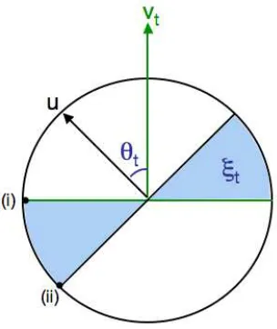
Figure 1: The projection of the error regionξt onto the plane defined by u and vt.
For a hypothesis vt, we will denote the angle between u and vtbyθt, and we will define the error
region of vt asξt={x∈S|SGN(vt·x)6=SGN(u·x)}. Figure 1 provides a schematic of the projection
of the error region onto the plane defined by u and vt.
We will use the term margin, in the context of learning half-spaces, to denote simply the distance from an example to the separator in question, as opposed to the standard use of this term (as the minimum over examples of this distance with respect to the target separator). For example, we will denote the margin of x with respect to v as|x·v|.
We will use a few useful inequalities forθon the interval(0,π2]. 4
π2 ≤
1−cosθ θ2 ≤
1
2, (1)
2
πθ≤sinθ ≤ θ. (2)
Equation (1) can be verified by checking that forθin this interval, 1−θcos2 θ is a decreasing function, and evaluating it at the endpoints.
We will also make use of the following lemma.
Lemma 4 For any fixed unit vector a and anyγ≤1,
γ 4≤Px∈S
|a·x| ≤√γ
d
≤γ.
The proof is deferred to the appendix.
4. A Lower Bound for the Perceptron Update
Pick some v0∈Rd. Repeat for t=0,1,2, . . .:
Get some (x,y) for which y(vt·x)≤0.
vt+1=vt+yx
On any update,
vt+1·u=vt·u+y(x·u). (3)
Thus, if we assume for simplicity that v0·u≥0 (we can always just start count when this first occurs) then vt·u≥0 always, andθt, the angle between u and vt is always acute. Sincekuk=1,
the following holds:
kvtkcosθt=vt·u.
The update rule also implies
kvt+1k2=kvtk2+1+2y(vt·x). (4)
Thuskvtk2≤t+kv0k2 for all t. In particular, this means that Theorem 1 is an immediate conse-quence of the following lemma.
Lemma 5 Assume v0·u≥0 (i.e., start count when this first occurs). Then
θt+1≤θt ⇒ sinθt≥min
1 3,
1 5kvtk
.
Proof Figure 1 shows the unit circle in the plane defined by u and vt. The dot product of any
point x∈Rd with either u or v
t depends only upon the projection of x into this plane. The point is
misclassified when its projection lies in the shaded region. For such points, y(u·x)is at most sinθt
(point (i)) and y(vt·x)is at least−kvtksinθt (point (ii)).
Combining this with Equations (3) and (4), we get
vt+1·u ≤ vt·u+sinθt,
kvt+1k2 ≥ kvtk2+1−2kvtksinθt.
To establish the lemma, we first assumeθt+1≤θtand sinθt≤5k1vtk, and then conclude that sinθt≥
1 3.
θt+1≤θt implies
cos2θt ≤ cos2θt+1 =
(u·vt+1)2 kvt+1k2 ≤
(u·vt+sinθt)2
kvtk2+1−2kvtksinθt
.
The final denominator is positive since sinθt≤5k1v
tk. Rearranging,
(kvtk2+1−2kvtksinθt)cos2θt ≤ (u·vt)2+sin2θt+2(u·vt)sinθt,
and usingkvtkcosθt = (u·vt):
Inputs: dimensionality d and budget on number of updates (mistakes) M.
Let v1=x1y1 for the first example (x1,y1). For t=1 to M:
Let (xt,yt) be the next example with y(x·vt)<0.
vt+1=vt−2(vt·xt)xt
Figure 2: The (non-active) modified Perceptron algorithm. The standard Perceptron update, vt+1= vt+ytxt, is in the same direction (note yt=−SGN(vt·xt)) but different magnitude (scaled
by a factor of 2|vt·xt|).
Again, since sinθt≤5k1vtk, it follows that(1−2kvtksinθt)≥35and that 2kvtksinθtcosθt≤25. Using
cos2=1−sin2, we then get
3
5(1−sin 2θ
t) ≤ sin2θt+
2 5,
which works out to sin2θt≥18, implying sinθt>13.
The problem is that the perceptron update can be too large. InR2 (e.g., Figure 1), whenθt is
tiny, the update will cause vt+1to overshoot the mark and swing too far to the other side of u, unless kvtkis very large: to be precise, we needkvtk=Ω(sin1θt). Butkvtkgrows slowly, at best at a rate
of√t. If sinθt is proportional to the error of vt, as in the case of data distributed uniformly over
the unit sphere, this means that the perceptron update cannot stably maintain an error rate≤εuntil t=Ω(1
ε2).
5. The Modified Perceptron Update
We now describe a modified Perceptron algorithm. Unlike the standard Perceptron, it ensures that vt·u is increasing, that is, the error of vt is monotonically decreasing. Another difference from the
standard update (and other versions) is that the magnitude of the current hypothesis,kvtk, is always
1, which is convenient for the analysis.
The modified Perceptron algorithm is shown in Figure 2. We now show that the norm of vtstays
at one. Note thatkv1k=1 and
kvt+1k2=kvtk2+4(vt·xt)2kxtk2−4(vt·xt)2=1
by induction. In contrast, for the standard perceptron update, the magnitude of vt increases steadily.
With the modified update, the error can only decrease, because vt·u only increases:
vt+1·u=vt·u−2(vt·xt)(xt·u) =vt·u+2|vt·xt||xt·u|. (5)
The second equality follows from the fact that vt misclassified xt. Thus vt·u is increasing, and
the increase can be bounded from below by showing that|vt·xt||xt·u|is large. This is a different
Hampson and Kibler (1999) previously used this update for learning linear separators, calling it the “Reflection” method, based on the “Reflexion” method due to Motzkin and Schoenberg (1954). These names are likely due to the following geometric property of this update:
xt·vt+1=xt·vt−2(xt·vt)(xt·xt) =−(xt·vt).
In general, one can consider modified updates of the form vt+1=vt−α(vt·xt)xt, which corresponds
to the “Relaxation” method of solving linear inequalities (Agmon, 1954; Motzkin and Schoenberg, 1954). Whenα6=2, the vectors vt no longer remain of fixed length; however, one can verify that
their corresponding unit vectors ˆvt satisfy
ˆ
vt+1·u= (vˆt·u+α|vˆt·xt||xt·u|)/
q
1−α(2−α)(vˆt·xt)2,
and thus any choice ofα∈[0,2]guarantees non-increasing error. Blum et al. (1996) usedα=1 to guarantee progress in the denominator (their analysis did not rely on progress in the numerator) as long as ˆvt·u and(vˆt·xt)2were bounded away from 0. Their approach was used in a batch setting
as one piece of a more complex algorithm for noise-tolerant learning. In our sequential framework, we can bound|vˆt·xt||xt·u|away from 0 in expectation, under the uniform distribution, and hence
the choice ofα=2 is most convenient, butα=1 would work as well. Although we do not further optimize our choice of the constantα, this choice itself may yield interesting future work, perhaps by allowing it to be a function of the dimension.
5.1 Analysis of (Non-Active) Modified Perceptron
How large do we expect|vt·xt|and|u·xt|to be for an error(xt,yt)? As we shall see, in d dimensions,
one expects each of these terms to be on the order of d−1/2sinθt, where sinθt =
p
1−(vt·u)2.
Hence, we might expect their product to be about (1−(vt·u)2)/d, which is how we prove the
following lemma.
Note, we have made little effort to optimize constant factors.
Lemma 6 For any vt, with probability at least 13,
1−vt+1·u≤(1−vt·u)
1− 1
50d
.
There exists a constant c>0, such that with probability at least 6364, for any vt,
1−vt+1·u≤(1−vt·u)
1−c
d
.
Proof We show only the first part of the lemma. The second part is quite similar. We will argue that each of|vt·xt|,|u·xt|is “small” with probability at most 1/3. This means, by the union bound,
that with probability at least 1/3, they are both sufficiently large.
The error rate of vt is θt/π, where cosθt = vt ·u. Also define the error region ξt =
{x∈S|SGN(vt·x)6=SGN(u·x)}. By Lemma 4, for an x drawn uniformly from the sphere,
Px∈S
|vt·x| ≤
θt
3π√d
Using P[A|B]≤P[A]/P[B], we have,
Px∈S
|vt·x| ≤
θt
3π√d
x∈ξt
≤ Px∈S[|vt·x| ≤ θt
3π√d]
Px∈S[x∈ξt] ≤
θt/(3π)
θt/π =1
3.
Similarly for|u·x|, and by the union bound the probability that x∈ξt is within margin 3πθ√d from
either u or v is at most 23. Since the updates only occur if x is in the error region, we now have a lower bound on the expected magnitude of|vt·x||u·x|:
Px∈S
|vt·x||u·x| ≥
θ2
t (3π√d)2
x∈ξt
≥13.
Hence, we know that with probability at least 1/3, |vt·x||u·x| ≥ 1−(vt·u)
2
100d ,since θt2≥sin2θt =
1−(vt·u)2and(3π)2<100.In this case,
1−vt+1·u ≤ 1−vt·u−2|vt·xt||u·xt|
≤ 1−vt·u−
1−(vt·u)2
50d
= (1−vt·u)
1−1+vt·u 50d
,
where the first inequality is by application of (5).
Finally, we give a high-probability bound, that is, Theorem 2, stated here with proof.
Theorem 7 With probability 1−δwith respect to the uniform distribution on the unit sphere, in the supervised, realizable setting, after M=O(d(log1ε+log1δ))mistakes, the generalization error of the modified Perceptron algorithm is at mostε.
Proof By the above lemma, we can conclude that, for any vector vt,
E[1−vt+1·u]≤(1−vt·u)
1− 1
3(50d)
.
This is because with≥1/3 probability it goes down by a factor of 1−50d1 and with the remaining ≤2/3 probability it does not increase. Hence, after M mistakes,
E[1−vM·u]≤(1−v1·u)
1− 1
150d M
≤
1− 1
150d M
,
since v1·u≥0. By Markov’s inequality, P
"
1−vM·u≥
1− 1
150d M
δ−1 #
≤δ.
Finally, using (1) and cosθM=vM·u, we see P[π42θ2M≥(1−150d1 )Mδ−1]≤δ. Using M=150d logεδ1 gives P[θMπ ≥ε]≤δ, as required.
The additional factor of 1ε in the bound on unlabeled samples ( ˜O(d
εlog1ε)) follows by upper
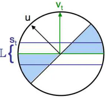
Figure 3: The active learning rule is to query for labels on points x inLwhich is defined by the threshold st on|vt·x|.
6. An Active Modified Perceptron
The ideal objective in designing an active learning rule that minimizes label complexity would be to query for labels only on points in the error region, ξt. However without knowledge of u,
the algorithm is unaware of the location of ξt. The intuition behind our active learning rule is
to approximate the error region, given the information the algorithm does have: vt. As shown in
Figure 3, the labeling regionLis simply formed by thresholding the margin of a candidate example with respect to vt.
The active version of the modified Perceptron algorithm is shown in Figure 4. The algorithm is similar to the algorithm of the previous section, in its update step. For its filtering rule, we maintain a threshold st and we only ask for labels of examples with |vt·x| ≤st. Approximating the error
region is achieved by choosing the threshold, st, adaptively, so as to manage the tradeoff between Lbeing too large, causing many labels to be wasted without hittingξt (and thus yielding updates),
andLonly containing points with very small margins with respect to vt, since our update step will
make very small updates on such points. We decrease the threshold adaptively over time, starting at s1=1/
√
d and reducing it by a factor of two whenever we have a run of labeled examples on which we are correct.
For Theorem 3, we select values of R,L that yieldεerror with probability at least 1−δ. The idea of the analysis is as follows:
Definition 7 We say the tth update is “good” if,
1−vt+1·u≤(1−vt·u)
1−c
d
.
(The constant c is from Lemma 6.)
1. (Lemma 8) First, we argue that st is not too small (we do not decrease st too quickly).
As-suming this is the case, then 2 and 3 hold.
Inputs: Dimensionality d, maximum number of labels L, and patience R.
v1=x1y1 for the first example (x1,y1). s1=1/
√
d For t=1 to L:
Wait for the next example x : |x·vt| ≤st and query its label.
Call this labeled example (xt,yt).
If (xt·vt)yt<0, then:
vt+1=vt−2(vt·xt)xt
st+1=st
else:
vt+1=vt
If predictions were correct on R consecutive labeled examples (i.e., (xi·vi)yi≥0 ∀i∈ {t−R+1,t−R+2, . . . ,t}),
then set st+1=st/2, else st+1=st.
Figure 4: An active version of the modified Perceptron algorithm.
mistakes total should not be much more than 32 times the number of updates we actually perform.
3. (Lemma 11) Each update is good (Definition 7) with probability at least 1/2.
4. (Theorem 3) Finally, we conclude that we cannot have too many label queries, updates, or total errors, because half of our updates are good, 1/32 of our errors are updates, and about 1/R of our labels are updates.
We first lower-bound st with respect to our error, showing that, with high probability, the
thresh-old st is never too small.
Lemma 8 With probability at least 1−L 34R, we have:
st≥
r
1−(u·vt)2
16d for t=1,2, . . . ,L, simultaneously. (6)
Before proving this lemma, it will be helpful to show the following lemma. As before, let us define ξt={x∈S|(x·vt)(x·u)<0}.
Lemma 9 For anyγ∈
0, q
1−(u·vt)2
4d
,
Pxt∈S
xt ∈ξt
|xt·vt|<γ
≥14.
Proof Let x be a random example from S such that |x·vt|<γ and, without loss of generality,
can decompose x=x′+ (x·vt)vt where x′=x−(x·vt)vt is the component of x orthogonal to vt, that
is, x′·vt=0. Similarly for u′=u−(u·vt)vt. Hence,
u·x= (u′+ (u·vt)vt)·(x′+ (x·vt)vt) =u′·x′+ (u·vt)(x·vt).
In other words, we err iff u′·x′ < −(u·vt)(x·vt). Using u·vt ∈ [0,1] and since x·vt ∈ [0,p
(1−(u·vt)2)/(4d)], we conclude that if
u′·x′<− r
1−(u·vt)2
4d , (7)
then we must err. Also, let ˆx′ = x′
kx′k be the unit vector in the direction of x′. It is straightforward
to check thatkx′k=p
1−(x·vt)2. Similarly, for u we define ˆu′= u
′
√ 1−(u·vt)2
. Substituting these
into (7), we must err if, ˆu′·xˆ′<−1/p
4d(1−(x·vt))2,and since
p
1−(x·vt)2≥
p
1−1/(4d), it suffices to show that,
Px∈S
" ˆ
u′·xˆ′<p −1 4d(1−1/(4d))
0≤x·vt≤γ
# ≥ 14.
What is the probability that this happens? Well, one way to pick x∈S would be to first pick x·vt
and then to pick ˆx′uniformly at random from the set S′={xˆ′∈S|xˆ′·vt =0}, which is a unit sphere
in one fewer dimensions. Hence the above probability does not depend on the conditioning. By Lemma 4, for any unit vector a∈S′, the probability that |uˆ′·a| ≤1/p4(d−1) is at most 1/2, so with probability at least 1/4 (since the distribution is symmetric), the signed quantity ˆu′·xˆ′< −1/p
4(d−1)<−1/p
4d(1−1/(4d)).
We are now ready to prove Lemma 8.
Proof [of Lemma 8] Suppose that condition (6) fails to hold for some t’s. Let t be the smallest number such that (6) fails. By our choice of s1, clearly t>1. Moreover, since t is the smallest such number, and u·vt is increasing, it must be the case that st =st−1/2, that is we just saw a run of R labeled examples(xi,yi), for i=t−R, . . . ,t−1, with no mistakes, vi=vt, and
si=2st <
r
1−(u·vt)2
4d =
r
1−(u·vi)2
4d . (8)
Such an event is highly unlikely, however, for any t. In particular, from Lemma 9, we know that the probability of (8) holding for any particular i and the algorithm not erring is at most 3/4. Thus the chance of having any such run of length R is at most L(3/4)R.
Lemma 9 also tells us something interesting about the fraction of errors that we are missing because we do not ask for labels. In particular,
Lemma 10 Given that st ≥
p
(1−(u·vt)2)/(16d), upon the tth update, each erroneous example
is queried with probability at least 1/32, that is,
Px∈S
|x·vt| ≤st
x∈ξt
Proof Using Lemmas 9 and 4, we have
Px∈S[x∈ξt∧ |x·vt| ≤st] ≥ Px∈S
"
x∈ξt∧ |x·vt| ≤
r
1−(u·vt)2
16d #
≥ 14Px∈S
"
|x·vt| ≤
r
1−(u·vt)2
16d #
≥ 1
64 q
1−(u·vt)2=
1 64sinθt
≥ 32πθt .
For the last inequality, we have used (2). However, Px∈S[x∈ξt] =θt/π, so we are querying an error
x∈ξt with probability at least 1/32, that is, the above inequality implies,
Px∈S
|x·vt| ≤st
x∈ξt
=Px∈S[x∈ξt∧ |x·vt| ≤st]
Px∈S[x∈ξt] ≥
θt/(32π)
θt/π = 1
32.
Next, we show that the updates are likely to make progress.
Lemma 11 Assuming that st ≥
p
(1−(u·vt)2)/(16d), a random update is good with probability
at least 1/2, that is,
Pxt∈S
h
(1−vt+1·u)≤(1−vt·u)
1−c
d
|x·vt| ≤st∧xt ∈ξt i
≥ 12.
Proof By Lemma 10, each error is queried with probability 1/32. On the other hand, by Lemma 6 of the previous section, 63/64 of all errors are good. Since we are querying at least 2/64 fraction of all errors, at least half of our queried errors must be good.
We now have the pieces to guarantee the convergence rate of the active algorithm, thereby proving Theorem 3. This involves bounding both the number of labels that we query as well as the number of total errors, which includes updates as well as errors that were never detected.
Theorem 3 With probability 1−δwith respect to the uniform distribution on the unit sphere, in the realizable setting, using L=O d log εδ1
(logdδ+log log1ε)
labels and making a total number of errors of O d log εδ1
(logdδ+log log1ε)
, the final error of the active modified Perceptron algorithm will beε, when run with the above L and R=O(logdδ+log log1ε).
Proof Let U be the number of updates performed. We know, by Lemma 8 that with probability 1−L(3
4)
R,
st ≥
sinθt
4√d ≥
θt
2π√d (9)
for all t. Again, we have used (2). By Lemma 11, we know that for each t which is an update, either (9) fails or
E[1−u·vt+1|vt]≤(1−u·vt)
1− c
2d
Hence, after U updates, using Markov’s inequality,
P
1−u·vL≥
4 δ
1− c
2d U
≤ δ4+L
3 4
R .
In other words, with probability 1−δ4−L(34)R, we also have
U≤2d c log
4
δ(1−u·vL) ≤
2d c log π2 δθ2 L =O d log 1
δε
,
where for the last inequality we used (1). In total, L≤R
U+log2s1
L
. This is because once every R labels we either have at least one update or we decrease sLby a factor of 2. Equivalently,
sL≤2U−L/R. Hence, with probability 1−δ4−L(34)R,
θL
2π√d ≤sL≤2
O(d log 1
δε)−L/R.
Working backwards, we choose L/R=Θ(d logεδ1)so that the above expression implies θLπ ≤ε, as required. We choose
R=10 log2L
δR =Θ log d logεδ1
δ !
=O
logd
δ+log log 1 ε
.
The first equality ensures that L(3
4)R ≤ δ4. Hence, for the L and R chosen in the theorem, with probability 1−34δ, we have error θLπ <ε. Finally, either condition (9) fails or each error is queried with probability at least 321. By the multiplicative Chernoff bound, if there were a total of E>64U errors, with probability ≥1−δ4, at least E/64>U would have been caught and used as updates. Hence, with probability at most 1−δ, we have achieved the target error using the specified number of labels and observing the specified number of errors.
7. Discussion and Conclusions
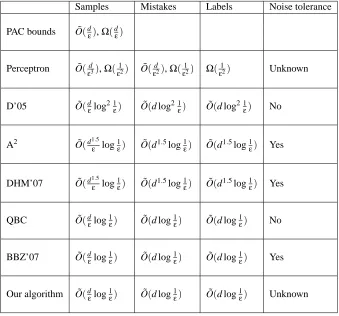
Samples Mistakes Labels Noise tolerance
PAC bounds O˜(d ε),Ω(dε)
Perceptron O˜(εd3),Ω( 1
ε2) O˜(
d ε2),Ω(
1
ε2) Ω( 1
ε2) Unknown
D’05 O˜(d
εlog2 1ε) O˜(d log2 1ε) O˜(d log2 1ε) No
A2 O˜(d1.5
ε log1ε) O˜(d1.5log1ε) O˜(d1.5log1ε) Yes
DHM’07 O˜(d1.5
ε log1ε) O˜(d1.5log1ε) O˜(d1.5log1ε) Yes
QBC O˜(d
εlog1ε) O˜(d log1ε) O˜(d log1ε) No
BBZ’07 O˜(dεlog1ε) O˜(d log1ε) O˜(d log1ε) Yes
Our algorithm O˜(d
εlog1ε) O˜(d log1ε) O˜(d log1ε) Unknown
In all these papers, the uniform distribution of data has consistently proved amenable to analysis. This is an impressive distribution to learn against because it is difficult in some ways—most of the data is close to the decision boundary, for instance—but a more common assumption would be to make the two classes Gaussian, or to merely stipulate that they are separated by a margin. As a modest step towards relaxing this distributional assumption, we can show an (at most) polynomial dependence of the label complexity onλ(Monteleoni, 2006), when the input distribution isλ-similar to uniform, a setting studied in Freund et al. (1997).
Our algorithm is in some ways fine-tuned for linearly-separable data that are distributed uni-formly; for instance, in the choice of the parameters R and s1. An immediate open problem is therefore the following:
1. Design a version of the algorithm that is sensible for general data distributions which may not be linearly separable.
2. What types of noise can be tolerated by this scheme?
3. For what distributions can its label complexity be analyzed?
A step towards the practical realization of our algorithm is the work of Monteleoni and K¨a¨ari¨ainen (2007), which applies a version of it to an optical character recognition problem.
Acknowledgments
This work was done while ATK was at the Toyota Technological Institute at Chicago. Much of this work was done while CM was visiting the Toyota Technological Institute at Chicago. Some of this work was done while CM was at the Massachusetts Institute of Technology, Computer Science and Intelligence Laboratory, and at the University of California, San Diego, Department of Computer Science and Engineering. CM would like to thank Adam Klivans, Brendan McMahan, and Vikas Sindhwani, for various discussions at TTI, and David McAllester for the opportunity to visit. The authors thank the anonymous reviewers of COLT 2005 and JMLR for helpful comments used in revision.
Appendix A. Proof of Lemma 4
Proof [Lemma 4] Let r=γ/√d and let Ad be the area of a d-dimensional unit sphere, that is, the
surface of a(d+1)-dimensional unit ball. Then
Px[|a·x| ≤r] = Rr
−rAd−2(1−z2)
d−2
2 (1−z2)−1/2dz
Ad−1
=2Ad−2
Ad−1
Z r
0
(1−z2)(d−3)/2dz. First observe,
r(1−r2)(d−3)/2≤
Z r
0
(1−z2)(d−3)/2dz≤r. (10) For x∈[0,0.5], 1−x≥4−x. Hence, for 0≤r≤2−1/2,
So we can conclude that the integral of (10) is in[r/2,r]for r∈[0,1/√d]. The ratio 2Ad−2/Ad−1 can be shown to be in the range[pd/3,√d]by straightforward induction on d, using the definition of theΓfunction, and the fact that Ad−1=2πd/2/Γ(d/2).
References
S. Agmon. The relaxation method for linear inequalities. Canadian Journal of Math., 6(3):382–392, 1954.
D. Angluin. Queries revisited. In Proc. 12th International Conference on Algorithmic Learning Theory, LNAI,2225:12–31, 2001.
M.-F. Balcan, A. Beygelzimer, and J. Langford. Agnostic active learning. In Proc. International Conference on Machine Learning, 2006.
M.-F. Balcan, A. Broder, and T. Zhang. Margin based active learning. In Proc. 20th Annual Con-ference on Learning Theory, 2007.
E.B. Baum. The perceptron algorithm is fast for nonmalicious distributions. Neural Computation, 2:248–260, 1997.
A. Blum, A. Frieze, R. Kannan, and S. Vempala. A polynomial-time algorithm for learning noisy linear threshold functions. In Proc. 37th Annual IEEE Symposium on the Foundations of Com-puter Science, 1996.
N. Cesa-Bianchi, A. Conconi, and C. Gentile. Learning probabilistic linear-threshold classifiers via selective sampling. In Proc. 16th Annual Conference on Learning Theory, 2003.
N. Cesa-Bianchi, C. Gentile, and L. Zaniboni. Worst-case analysis of selective sampling for linear-threshold algorithms. In Advances in Neural Information Processing Systems 17, 2004.
D.A. Cohn, L. Atlas, and R.E. Ladner. Improving generalization with active learning. Machine Learning, 15(2):201–221, 1994.
S. Dasgupta. Analysis of a greedy active learning strategy. In Advances in Neural Information Processing Systems 17, 2004.
S. Dasgupta. Coarse sample complexity bounds for active learning. In Advances in Neural Infor-mation Processing Systems 18, 2005.
S. Dasgupta, D. Hsu, and C. Monteleoni. A general agnostic active learning algorithm. In Advances in Neural Information Processing Systems, 2007.
Y. Freund, H.S. Seung, E. Shamir, and N. Tishby. Selective sampling using the query by committee algorithm. Machine Learning, 28(2-3):133–168, 1997.
S. Hampson and D. Kibler. Minimum generalization via reflection: A fast linear threshold learner. Machine Learning, 37(1):51–73, 1999.
S. Hanneke. A bound on the label complexity of agnostic active learning. In Proc. International Conference on Machine Learning, 2007.
M. K¨a¨ari¨ainen. Active learning in the non-realizable case. In Proc. 17th International Conference on Algorithmic Learning Theory, 2006.
D.D. Lewis and W.A. Gale. A sequential algorithm for training text classifiers. In Proc. of SIGIR-94, 17th ACM International Conference on Research and Development in Information Retrieval, 1994.
C. Monteleoni and M. K¨a¨ari¨ainen. Practical online active learning for classification. In Proc. of the IEEE Conference on Computer Vision and Pattern Recognition, Online Learning for Classifica-tion Workshop, 2007.
C.E. Monteleoni. Learning with Online Constraints: Shifting Concepts and Active Learning. PhD Thesis, MIT Computer Science and Artificial Intelligence Laboratory, 2006.
T.S. Motzkin and I.J. Schoenberg. The relaxation method for linear inequalities. Canadian Journal of Math., 6(3):393–404, 1954.
F. Rosenblatt. The perceptron: A probabilistic model for information storage and organization in the brain. Psychological Review, 65:386–407, 1958.
R.A. Servedio. On PAC learning using winnow, perceptron, and a perceptron-like algorithm. In Computational Learning Theory, pages 296 – 307, 1999.
H.S. Seung, M. Opper, and H. Sompolinsky. Query by committee. In Proc. Fifth Annual ACM Conference on Computational Learning Theory, 1992.