Particle Swarm Model Selection

Particle Swarm Model Selection

Hugo Jair Escalante [email protected]

Manuel Montes [email protected]

Luis Enrique Sucar [email protected]

Department of Computational Sciences

National Institute of Astrophysics, Optics and Electronics Puebla, M´exico, 72840

Editor: Isabelle Guyon and Amir Saffari

Abstract

This paper proposes the application of particle swarm optimization (PSO) to the problem of full

model selection, FMS, for classification tasks. FMS is defined as follows: given a pool of

pre-processing methods, feature selection and learning algorithms, to select the combination of these that obtains the lowest classification error for a given data set; the task also includes the selection of hyperparameters for the considered methods. This problem generates a vast search space to be explored, well suited for stochastic optimization techniques. FMS can be applied to any classifi-cation domain as it does not require domain knowledge. Different model types and a variety of algorithms can be considered under this formulation. Furthermore, competitive yet simple models can be obtained with FMS. We adopt PSO for the search because of its proven performance in different problems and because of its simplicity, since neither expensive computations nor com-plicated operations are needed. Interestingly, the way the search is guided allows PSO to avoid overfitting to some extend. Experimental results on benchmark data sets give evidence that the proposed approach is very effective, despite its simplicity. Furthermore, results obtained in the framework of a model selection challenge show the competitiveness of the models selected with

PSO, compared to models selected with other techniques that focus on a single algorithm and that

use domain knowledge.

Keywords: full model selection, machine learning challenge, particle swarm optimization, exper-imentation, cross validation

1. Introduction

of hyperparameters for the considered methods, resulting in a vast search space that is well suited for stochastic optimization techniques.

Adopting a broader interpretation to the model selection problem allows us to consider different model types and a variety of methods, in contrast to techniques that consider a single model type (i.e., either learning algorithm or feature selection method, but not both) and a single method (e.g., neural networks). Also, since neither prior domain knowledge nor machine learning knowledge is required, FMS can be applied to any classification problem without modification. This is a clear advantage over ad-hoc model selection methods that perform well on a single domain or that work for a fixed algorithm. This will help users with limited machine learning knowledge, since FMS can be seen as a black-box tool for model selection. Machine learning experts can also benefit from this approach. For example, several authors make use of search strategies for the selection of candidate models (Lutz, 2006; Boull´e, 2007; Reunanen, 2007; Wichard, 2007), the FMS approach can be adopted for obtaining such candidate models.

One could expect a considerable loss of accuracy by gaining generality. However, this is not the case of the proposed approach since in international competitions it showed comparable per-formance to other techniques that were designed for a single algorithm (i.e., doing hyperparameter optimization) and to methods that took into account domain knowledge (Guyon et al., 2008). The main drawback is the computational cost to explore the vast search space, particularly for large data sets. But, we can gain efficiency without a significant loss in accuracy, by adopting a random subsampling strategy, see Section 4.3. The difficult interpretability of the selected models is an-other limitation of the proposed approach. However, naive users may accept to trade interpretably for ease-of-use, while expert users may gain insight in the problem at hand by analyzing the struc-ture of the selected model (type of preprocessing chosen, number of feastruc-tures selected, linearity or non-linearity of the predictor).

In this paper, we propose to use particle swarm optimization (PSO) for exploring the full-models search space. PSO is a bio-inspired search technique that has shown comparable performance to that of evolutionary algorithms (Angeline, 1998; Reyes and Coello, 2006). Like evolutionary algorithms, PSO is useful when other techniques such as gradient descend or direct analytical discovery are not applicable. Combinatoric and real-valued optimization problems in which the optimization surface possesses many locally optimal solutions, are well suited for swarm optimization. In FMS it must be found the best combination of methods (for preprocessing, feature selection and learning) and simultaneously optimizing real valued functions (finding pseudo-optimal parameters for the considered methods), in consequence, the application of PSO is straightforward.

computational cost (Gudise and Venayagamoorthy, 2003; Hern´andez et al., 2004; Xiaohui et al., 2003; Yoshida et al., 2001; Robinson, 2004; Kennedy and Eberhart, 2001; Reyes and Coello, 2006). PSO is compared to pattern search (PS) in order to evaluate the added value of using the swarm strategy instead of another intensive search method. We consider PS among other search techniques because of its simplicity and proved performance in model selection (Momma and Bennett, 2002; Bi et al., 2003; Dennis and Torczon, 1994). Cross validation (CV) is used in both techniques for assessing the goodness of models. Experimental results in benchmark data give evidence that both PSO and PS are effective strategies for FMS. However, it was found that PSO outperforms PS, showing better convergence behavior and being less prone to overfitting. Furthermore, the proposed method was evaluated in the context of a model selection competition in which several specialized and prior-knowledge based methods for model selection were used. Models selected with PSO were always among the top ranking models through the different stages of the challenge (Guyon et al., 2006c, 2007, 2008; Escalante et al., 2007). During the challenge, our best entry was ranked 8thover all ranked participants, 5th among the methods that did not use domain knowledge and 2nd among the methods that used the software provided by the organizers (Guyon et al., 2006c, 2007, 2008). In this paper we outperform the latter entry while reducing the computational burden by using a subsampling strategy; our best entry is currently the top-ranked one among models that do not use prior domain knowledge and 2nd _{over all entries, see Section 4.3.}

PSO has been widely used for parameter selection in supervised learning (Kennedy and Eber-hart, 1995, 2001; Salerno, 1997; Gudise and Venayagamoorthy, 2003). However, parameter selec-tion is related with the first level of inference in which, given a learning algorithm, the task is to find parameters for such algorithm in order to describe the data. For example, in neural networks the adjustment of weights between units according to some training data is a parameter selection prob-lem. Hyperparameter optimization, on the other hand, is related with the second level of inference, that is, finding parameters for the methods that in turn should determine parameters for describ-ing the data. In the neural network example, selectdescrib-ing the optimal number of units, the learndescrib-ing rate, and the number of epochs for training the network is a hyperparameter optimization problem. FMS is capable of operating across several levels of inference by simultaneously performing feature selection, preprocessing and classifier selection, and hyperparameter optimization for the selected methods. PSO has been used for hyperparameter optimization by Voss and Feng (2002), however they restricted the problem to linear systems for univariate data sets, considering one hundred data observations. In this paper we are going several steps further: we applied PSO for FMS considering non-linear models in multivariate data sets with a large number of observations.

The main contribution of this work is experimental: we provide empirical evidence indicating that by using PSO we were able to perform intensive search over a huge space and succeeded in selecting competitive models without significantly overfitting. This is due to the way the search is guided in PSO: performing a broad search around promising solutions but not overdoing in terms of really fine optimization. This sort of search is known to help avoiding overfitting by undercomput-ing (Dietterich, 1995). Experimental results supported by some a posteriori analysis give evidence of the validity of our approach. The way we approached the model selection problem and the use of a stochastic-search strategy are also contributions. To the best of our knowledge there are no similar works that consider the FMS problem for classification tasks.

The rest of this paper is organized as follows. In the next section we describe the general PSO algorithm. In Section 3, we describe the application of PSO to FMS. Section 4 presents experimental results in benchmark data; comparing the performance of PSO to that of PS in FMS and analyzing the performance of PSO under different parameter settings; also, are described the results obtained in the framework of a model selection competition. In Section 5, we analyze mechanisms in PSMS that allow to select competitive models without overfitting the data. Finally, in Section 6, we present the conclusions and outline future research directions.

2. Particle Swarm Optimization (PSO)

PSO is a population-based search algorithm inspired by the behavior of biological communities that exhibit both individual and social behavior; examples of these communities are flocks of birds, schools of fishes and swarms of bees. Members of such societies share common goals (e.g., find-ing food) that are realized by explorfind-ing its environment while interactfind-ing among them. Proposed by Kennedy and Eberhart (1995), PSO has become an established optimization algorithm with applica-tions ranging from neural network training (Kennedy and Eberhart, 1995; Salerno, 1997; Kennedy and Eberhart, 2001; Gudise and Venayagamoorthy, 2003; Engelbrecht, 2006) to control and engi-neering design (Hern´andez et al., 2004; Xiaohui et al., 2003; Yoshida et al., 2001; Robinson, 2004). The popularity of PSO is due in part to the simplicity of the algorithm (Kennedy and Eberhart, 1995; Reyes and Coello, 2006; Engelbrecht, 2006), but mainly to its effectiveness for producing good re-sults at a very low computational cost (Gudise and Venayagamoorthy, 2003; Kennedy and Eberhart, 2001; Reyes and Coello, 2006). Like evolutionary algorithms, PSO is appropriate for problems with immense search spaces that present many local minima.

In PSO each solution to the problem at hand is called a particle. At each time t, each particle, i, has a position xt_i=<xt_i,1,xt_i,2, . . . ,xt_i,d>in the search space; where d is the dimensionality of the solutions. A set of particles S={xt₁,xt₂, . . . ,xt

m} is called a swarm. Particles have an associated

velocity value that they use for flying (exploring) through the search space. The velocity of particle i at time t is given by vt_i=<vt_i,1,vt_i,2, . . . ,vt_i,d>, where vt_i,kis the velocity for dimension k of particle i at time t. Particles adjust their flight trajectories by using the following updating equations:

vt_i,+_j1=W×vt_i,j+c1×r1×(pi,j−xti,j) +c2×r2×(pg,j−xti,j), (1)

xt_i+_,j1=xt_i,j+vt_i,+_j1 (2)

where pi,j is the value in dimension j of the best solution found so far by particle i; pi =<

pi,1, . . . ,pi,d>is called personal best. pg,j is the value in dimension j of the best particle found

piand pgeach particle i takes into account individual (local) and social (global) information for

up-dating its velocity and position. In that respect, c1,c2∈Rare constants weighting the influence of

local and global best solutions, respectively. r1,r2∼ U[0,1]are values that introduce randomness

into the search process. W is the so called inertia weight, whose goal is to control the impact of the past velocity of a particle over the current one, influencing the local and global exploration abilities of the algorithm. This is one of the most used improvements of PSO for enhancing the rate of con-vergence of the algorithm (Shi and Eberhart, 1998, 1999; van den Bergh, 2001). For this work we considered an adaptive inertia weight specified by a triplet W= (wstart,wf,wend); where wstart and

wend are the initial and final values for W , respectively, and wf indicates the fraction of iterations

in which W is decreased. Under this setting W is decreased by W=W−wdec from iteration t=1 (where W =wstart) up to iteration t=I×wf (after which W =wend); where wdec=wstart_I×−_ww_fend and

I is the maximum number of iterations. This setting allows us to explore a large area at the start of the optimization, when W is large, and to slightly refine the search later by using a smaller inertia weight (Shi and Eberhart, 1998, 1999; van den Bergh, 2001).

An adaptive W can be likened to the temperature parameter in simulated annealing (Kirkpatrick et al., 1983); this is because, in essence, both parameters influence the global and local exploration abilities of their respective algorithms, although in different ways. A constant W is analogous to the momentum parameter p in gradient descend with momentum term (Qian, 1999), where weights are updated by considering both the current gradient and the weight change of the previous step (weighed by p). Interestingly, the inertia weight is also similar to the weight-decay constant (γ) used in machine learning to prevent overfitting. In neural networks the weights are decreased by (1−γ)in each learning step, which is equivalent to add a penalty term into the error function that encourages the magnitude of the weights to decay towards zero (Bishop, 2006; Hastie et al., 2001); the latter penalizes complex models and can be used to obtain sparse solutions (Bishop, 2006).

The pseudo code of the PSO algorithm considered in this work is shown in Algorithm 1; default recommended values for the FMS problem are shown as well (these values are based on the analysis of Section 2.1 and experimental results from Section 4.2). The swarm is randomly initialized, considering restrictions on the values that each dimension can take. Next, the goodness of each particle is evaluated and p_g, p_1,...,m are initialized. Then, the iterative PSO process starts, in each iteration: i)the velocities and positions of each particle in every dimension are updated according to Equations (1) and (2); ii)the goodness of each particle is evaluated; iii)p_gand p_1,...,mare updated, if needed; and iv)the inertia weight is decreased. This process is repeated until either a maximum number of iterations is reached or a minimum fitness value is obtained by a particle in the swarm (we used the first criterion for FMS); eventually, an (locally) optimal solution is found.

A fitness function is used to evaluate the aptitude (goodness) of candidate solutions. The def-inition of a specific fitness function depends on the problem at hand; in general it must reflect the proximity of the solutions to the optima. A fitness function F :Ψ→R, whereΨis the space of particles positions, should return a scalar fxifor each particle position xi, indicating how far particle

i is from the optimal solution to the problem at hand. For FMS the goal is to improve classification accuracy of full models. Therefore, any function F, which takes as input a model and returns an estimate of classification performance, is suitable (see Section 3.3).

Algorithm 1 Particle swarm optimization.

Require: [Default recommended values for FMS] – c1,c2: individual/social behavior weights;[c1=c2=2]

– m: swarm size;[m=5]

– I: number of iterations;[I=50]

– F(Ψ→R): fitness function; [F(Ψ→R) =2−fold CV BER ] – W: Inertia weight W = (1.2, 0.5, 0.4)

Set decrement factor for W (wdec=wstart−_I×ww_fend)

Initialize swarm (S={x1,x2, . . . ,xm})

Compute fx1,...,m=F(x1,...,m)(Section 3.3)

Locate leader (p_g) and set personal bests (p_1,...,m=x1,...,m)

t=1

while t<I do for all xi∈S do

Calculate velocity vifor xi(Equation (1))

Update position of xi(Equation (2))

Compute fxi=F(xi)

Update p_i(if necessary) end for

Update pg(if necessary)

if t<⌊I×wf⌋then

W =W−wdec

end if t++ end while return p_g

Kennedy and Eberhart, 2001; Engelbrecht, 2006). With this topology, however, the swarm is prone to converge to local minima. We tried to overcome this limitation by using the adaptive inertia weight, W .

2.1 PSO Parameters

Selecting the best parameters(W,c1,c2,m,I)for PSO is another model selection task. In the

We will start analyzing c1,c2∈R, the weighting factors for individual and social behavior. It

has been shown that convergence is guaranteed1 for PSO under certain values of c1,c2 (van den

Bergh, 2001; Reyes and Coello, 2006; Ozcan and Mohan, 1998; Clerc and Kennedy, 2002). Most convergence studies have simplified the problem to a single one-dimensional particle, settingφ= c1×r1+c2×r2, and pgand piconstant (van den Bergh, 2001; Reyes and Coello, 2006; Ozcan and

Mohan, 1998; Clerc and Kennedy, 2002). A complete study including the inertia weight is carried out by van den Bergh (2001). In agreement with this study the valueφ<3.8 guarantees eventual convergence of the algorithm when the inertia weight W is close to 1.0. For the experiments in this work it was fixed c1=c2=2, with these values we haveφ<3.8 with high probability P(φ<3.8)≈

0.9, given the uniformly distributed numbers r1,r2(van den Bergh, 2001). The configuration c1=

c2=2 also has been proven, empirically, to be an effective choice for these parameters (Kennedy

and Eberhart, 1995; Shi and Eberhart, 1998, 1999; Kennedy and Mendes, 2002).

Note, however, the restriction that W remains close to 1.0. In our experiments we considered a value of W =1.2 at the beginning of the search, decreasing it during 50% (i.e., wf =0.5) of the

PSO iterations up to the value W =0.4. In consequence, it is possible that at the end of the search process the swarm may show divergent behavior. In practice, however, the latter configuration for W resulted very useful for FMS, see Section 4. This selection of W should not be surprising since even the configuration W= (1,1,0) has obtained better results than using a fixed W in empirical studies (Shi and Eberhart, 1998). Experimental results with different configurations of W for FMS give evidence that the configuration we selected can provide better models than using constant W, see Section 4.2; although further experiments need to be performed in order to select the best W configuration for FMS.

With respect to m, the size of the swarm, experimental results suggest that the size of the popu-lation does not damage the performance of PSO (Shi and Eberhart, 1999), although slightly better results have been obtained with a large value of m, (Shi and Eberhart, 1999). Our experimental results in Section 4.2 confirm that the selection of m is not crucial, although (contrary to previous results) slightly better models are obtained by using a small swarm size. The latter is an important result for FMS because using a small number of particles reduces the number of fitness function evaluations, and in consequence the computational cost of the search.

Regarding the number of iterations, to the best of our knowledge, there is no work on the subject. This is mainly due to the fact that this issue depends mostly on the complexity of the problem at hand and therefore a general rule cannot be derived. For FMS the number of iterations should not be large to avoid oversearching (Dietterich, 1995). For most experiments in this paper we fixed I=100. However, experimental results in Section 4.2 show that by running PSO for a smaller number of iterations is enough to obtain models of the same, and even better, generalization performance. This gives evidence that early stopping can be an useful mechanism to avoid overfitting, see Section 5.

3. Particle Swarm Model Selection

Since one of the strong advantages of PSO is its simplicity, its application to FMS is almost di-rect. Particle swarm full model selection (hereafter PSMS, that is the application of PSO to FMS) is

1. Note that in PSO we say that the swarm converges iff limt→infpgt=p, where p is an arbitrary position in the search

ID Object name F Hyperparameters Description

1 Ftest FS fmax, wmin, pval, f drmax Feature ranking according the F-statistic

2 Ttest FS fmax, wmin, pval, f drmax Feature ranking according the T-statistic

3 aucfs FS fmax, wmin, pval, f drmax Feature ranking according to the AUC criterion

4 odds-ratio FS fmax, wmin, pval, f drmax Feature ranking according to the odds ratio statistic

5 relief FS fmax, wmin, knum Relief ranking criterion

6 rffs FS fmax, wmin Random forest used as feature selection filter

7 svcrfe FS fmax Recursive feature elimination filter using svc

8 Pearson FS fmax, wmin, pval, f drmax Feature ranking according to the Pearson correlation coef.

9 ZFilter FS fmax, wmin Feature ranking according to a heuristic filter

10 gs FS fmax Forward feature selection with Gram-Schmidt orth.

11 s2n FS fmax, wmin Signal-to-noise ratio for feature ranking

12 pc−extract FS fmax Extraction of features with PCA

1 normalize Pre center Normalization of the lines of the data matrix

2 standardize Pre center Standardization of the features

3 shi f t−scale Pre takelog Shifts and scale data

1 bias Pos none Finds the best threshold for the output of the classifiers

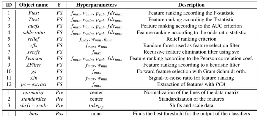
Table 1: Feature selection (FS), preprocessing (Pre) and postprocessing (Pos) objects available in CLOP. A brief description of the methods and their hyperparameters is presented.

described by the pseudocode in Algorithm 1, in this section are presented additional details about PSMS: first we describe the pool of methods considered in this work; then, we describe the rep-resentation of particles and the fitness function used; finally, we briefly discuss complexity is-sues. The code of PSMS is publicly available from the following website http://ccc.inaoep. mx/˜hugojair/code/psms/.

3.1 The Challenge Learning Object Package

In order to implement PSMS we need to define the models search space. For this purpose we con-sider the set of methods in a machine learning toolbox from which full models can be generated. Currently, there are several machine learning toolboxes, some of them publicly available (Franc and Hlavac, 2004; van der Heijden et al., 2004; Wichard and Merkwirth, 2007; Witten and Frank, 2005; Saffari and Guyon, 2006; Weston et al., 2005); even there is a track of this journal (JMLR) dedi-cated to machine learning software. This is due to the increasing interest from the machine learning community in the dissemination and popularization of this research field (Sonnenburg, 2006). The Challenge Learning Object Package2(CLOP) is one of such development kits distributed under the GNU license (Saffari and Guyon, 2006; Guyon et al., 2006c, 2007, 2008). CLOP is a MatlabR

tool-box with implementations of feature-variable selection methods and machine learning algorithms (CLOP also includes the PSMS implementation used in this work). The list of available prepro-cessing, feature selection and postprocessing methods in the CLOP toolbox is shown in Table 1; a description of the learning algorithms available in CLOP is presented in Table 2. One should note that this version of CLOP includes the methods that best performed in a model selection competition (Guyon et al., 2008; Cawley and Talbot, 2007a; Lutz, 2006).

ID Object name Hyperparameters Description

1 zarbi none Linear classifier

2 naive none Na¨ıve Bayes

3 klogistic none Kernel logistic regression

4 gkridke none Generalized kridge (VLOO)

5 logitboost units number, shrinkage, depth Boosting with trees (R)

6 neural units number, shrinkage, maxiter, balance Neural network (Netlab)

7 svc shrinkage, kernel parameters (coef0, degree, gamma) SVM classifier

8 kridge shrinkage, kernel parameters (coef0, degree, gamma) Kernel ridge regression

9 rf units number, balance, mtry Random forest (R)

10 lssvm shrinkage, kernel parameters (coef0, degree, gamma), balance Kernel ridge regression

Table 2: Available learning objects with their respective hyperparameters in the CLOP package.

In consequence, for PSMS the pool3 of methods to select from are those methods described in Tables 1 and 2. In CLOP a typical model consists of the chain, which is a grouping object that allows us to perform serial concatenation of different methods. A chain may include combinations of (several/none) feature selection algorithm(s) followed by (several/none) preprocessing method(s), in turn followed by a learning algorithm and finally (several/none) postprocessing algorithm(s). For example, the model given by:

chain{gs( f max=8),standardize(center=1),neural(units=10,s=0.5,balance=1,iter=10)}

uses gs for feature selection, standardization of data and a balanced neural network classifier with 10 hidden units, learning rate of 0.5, and trained for 10 iterations. In this work chain objects that include methods for preprocessing, feature selection and classification are considered full-models. Specifically, we consider models with at most one feature selection method, but allowing to perform preprocessing before feature selection and viceversa, see Section 3.2. The bias method was used as postprocessing in every model tested to set an optimal threshold in the output of the models in order to minimize their error. The search space in FMS is given by all the possible combinations of methods and hyperparameters; an infinite search space due to the real valued parameters.

3.2 Representation

In PSO each potential solution to the problem at hand is considered a particle. Particles are rep-resented by their position, which is nothing but a d−dimensional numerical vector (d being the dimensionality of the solution). In FMS potential solutions are full-models, in consequence, for PSMS we need a way to codify a full-model by using a vector of numbers. For this purpose we propose the representation described in Equation (3), the dependence on time (t) is omitted for clarity.

xi=<xi,pre,yi,1...Npre,xi,f s,yi,1,...Nf s,xi,sel,xi,class,yi,1,...Nclass> (3)

where xi,pre∈ {1, . . . ,8}represents a combination of preprocessing methods. Each combination is

represented by a binary vector of size 3 (i.e., the number of preprocessing methods considered), there are 23=8 possible combinations. Each element of the binary vector represents a single pre-processing method; if the value of the kthelement is set to 1 then the preprocessing method with ID = k is used (see Table 1). For example, the first combination<0,0,0>means no preprocessing; while the seventh<1,1,0>means that this model (xi) uses normalization and standardization as

preprocessing. yi,1...Npre codify the hyperparameters for the selected combination of preprocessing

methods, Npre=3 because each preprocessing method has a single hyperparameter; note that the

order of the preprocessing methods is fixed (i.e., standardization can never be performed before normalization), in the future we will relax this constraint. xi,f s∈ {0, . . . ,12}represents the ID of

the feature selection method used by the model (see Table 1), and yi,1...Nf s its respective

hyperpa-rameters; Nf sis set to the maximum number of hyperparameters that any feature selection method

can take. xi,sel is a binary variable that indicates whether preprocessing should be performed before

feature selection or viceversa. xi,class∈ {1, . . . ,10}represents the classifier selected and yi,1,...Nclass

its respective hyperparameters; Nclassis the maximum number of hyperparameters that a classifier

can take. This numerical codification must be decoded and used with the chain grouping object for obtaining a full-model from a particle position xi. Note that the dimensionality of each particle is

d=1+Npre+1+Nf s+1+1+Nclass=16.

3.3 Fitness Function

In FMS it is of interest to select models that minimize classification errors on unseen data (i.e., maximizing generalization performance). Therefore, the fitness function (F) should relate a model with an estimate of its classification performance in unseen data. The simplicity of PSMS allows us to use any classification performance measure as F, because the method does not require derivatives. Thus, valid options for F include mean absolute error, balanced error rate, squared root error, recall, precision, area under the ROC curve, etcetera. For this work it was used the balanced error rate (BER) as F. BER takes into account misclassification rates in both classes, which prevents PSMS of selecting biased models (favoring the majority class) in imbalanced data sets. Furthermore, BER has been used in machine learning challenges as leading error measure for ranking participants (Guyon et al., 2007, 2008). The BER of modelψis the average of the misclassifications obtained byψover the classes in a data set, as described in Equation (4):

BER(ψ) =E++E−

2 (4)

where E+and E−are the misclassifications rates for the positive and negative classes, respectively.

3.4 Computational Complexity

As we have seen, the search space in the FMS problem is composed by all the possible models that can be built given the considered methods and their hyperparameters. This is an infinite search space even with the restriction imposed to the values that models can take; this is the main drawback of FMS. However, the use of particle swarm optimization (PSO) allows us to harness the complexity of this problem. Most algorithms used for FMS cannot handle very big search spaces. But PSO is well suited to large search spaces: it converges fast and has a manageable computational complexity (Kennedy and Eberhart, 2001; Reyes and Coello, 2006). As we can see from Algorithm 1, PSO is very simple and does not involve expensive operations.

The computational expensiveness of PSMS is due to the fitness function we used. For each selected model the fitness function should train and evaluate such model k−times. Depending on the model complexity this process can be performed on linear, quadratic or higher order times. Clearly, computing the fitness function using the entire training set, as opposed to k-fold CV, could reduce PSMS complexity, although we could easily overfit the data. For a single run of PSMS the fitness function should be evaluatedρ=m×(I+1)times, with m being the swarm size and I the number of iterations. Suppose the computational complexity of model λis bounded by λO then

the computational complexity of PSMS will be bounded byρ×k×λO. Because λOis related to

the computational complexity of model λ (which depends on the size and dimensionality of the data set) this value may vary dramatically. For instance, computing the fitness function for a na¨ıve Bayes model in a high dimensional data set takes around two seconds4, whereas computing the same fitness function for the same data set could take several minutes if a support vector classifier is used.

In order to reduce the computational cost of PSMS we could introduce a complexity penalty-term into the fitness function (this is current work). A simpler alternative solution is calculating the fitness function for each model using only a small subset of the available data; randomly selected and different each time. This approach can also be useful for avoiding local minima. The subsampling heuristic was used for high-dimensional data sets and for data sets with a large number of examples. Experimental results show an important reduction of processing time, without a significant loss of accuracy, see Section 4.3. We emphasize that complexity is due to the nature of the FMS problem. With this approach, however, users will be able to obtain models for their data without requiring knowledge on the data or on machine learning techniques.

4. Experimental Results

In this section results of experiments with PSMS using benchmark data from two different sources are presented. First, we present results on a suite of benchmark machine learning data sets5used by several authors (Mika et al., 2000; R¨atsch et al., 2001; Cawley and Talbot, 2007b); such data sets are described in Table 3, ten replications (i.e., random splits of training and testing data) of each data set were considered. These data sets were used to compare PSO to PS in the FMS problem (Section 4.1) and to study the performance of PSMS under different settings (Section 4.2). Next we applied PSMS to the data sets used in a model selection competition (Section 4.3). The goal of the latter experiments is to compare the performance of PSMS against other model selection strategies.

4. Most of the experiments were carried out on a workstation with PentiumT M4 processor at 2.5 GHz, and 1 gigabyte in RAM.

ID Data set Training Patterns

Testing Patterns

Input Fea-tures

1 Breast cancer 200 77 9

2 Diabetes 468 300 8

3 Flare solar 666 400 9

4 German 700 300 20

5 Heart 170 100 13

6 Image 1300 1010 20

7 Splice 1000 2175 60

8 Thyroid 140 75 5

9 Titanic 150 2051 3

Table 3: Data sets used in the comparison of PSO and PS, ten replications (i.e., random splits of training and testing sets) for each data set were considered.

4.1 A Comparison of PSO and PS

In the first set of experiments we compared the performance of PSO to that of another search strategy in the FMS problem. The goal was to evaluate the advantages of using the swarm strategy over another intensive search method. Among the available search techniques we selected PS because of its simplicity and proved performance in model selection (Dennis and Torczon, 1994; Momma and Bennett, 2002; Bi et al., 2003). PS is a direct search method that samples points in the search space in a fixed pattern about the best solution found so far (the center of the pattern). Fitness values are calculated for the sampled points trying to find a minimizer; if a new minimum is find then the center of the pattern is changed, otherwise the search step is reduced by half; this process is iterated until a stop criteria is met. The considered PS algorithm described in Algorithm 2 is an adaptation of that proposed by Momma et al. for hyperparameter optimization of support vector regression (Momma and Bennett, 2002; Bi et al., 2003).

The input to PS is the pattern P and the search step ∆. Intuitively, P specifies the direction of the neighboring solutions that will be explored; while∆specifies the distance to such neighboring solutions. There are several ways to generate P; for this work we used the nearest neighbor sampling pattern (Momma and Bennett, 2002). Such pattern is given numerically by P= [Id −Id 0T1×d],

where Id is the identity matrix of size d; 01×dis a vector of size 1×d with all zero entries; d is the

dimensionality of the problem. ∆, a vector of size 1×d, is the search step by which the space of solutions is explored. We defined∆= qmaxvals−qminvals

2 , where qmaxvals and qminvals are the maximum

and minimum values that the solutions can take, respectively. Each iteration of PS involves the evaluation of Nc−1 solutions (where Ncis the number of columns of P). Solutions are updated by

adding sj( j∈1, . . . ,Nc−1) to the current-best solution qg; where each sjis obtained by multiplying

(element-by-element) the search step vector ∆and the jth column of P. q_g is replaced by a new solution q_j only if fq_j < fmin= fqg. The output of PS is qg, the solution with the lowest fitness

value; we encourage the reader to follow the references for further details (Momma and Bennett, 2002; Dennis and Torczon, 1994).

Algorithm 2 Pattern search. piis the ithcolumn of P, Ncthe number of columns in P.

Require:

– Ips: number of iterations

– F(Ψ→R): fitness function – P: pattern

–∆: search step

Initialize solution q_i(i=1) Compute fq_i=F(q_i)(Section 3.3) Set q_g=q_i; fmin= fqi

while i<Ipsdo

for all pj∈P1,...,Nc−1do

sj=∆.pj

q_j=q_g+sj

Compute fq_j=F(qj)

if fqj< fminthen

Update q_g(q_g=q_j, fmin= fqj) end if

i++ end for

∆=∆/2 end while return q_g

representation, fitness function and restrictions on the values that each dimension can take were considered for both methods, see Section 3. Under these settings PS is a very competitive baseline for PSO.

In each experiment described below, we let PS and PSO perform the same number of fitness function evaluations, using exactly the same settings and data sets, guaranteeing a fair comparison. Since both methods use the same fitness function and perform the same number of fitness function evaluations, the difference in performance indicates the gain we have by guiding the search accord-ing to Equations (1) and (2). As recommended by Demsar, we used the Wilcoxon signed-rank test for the comparison of the resultant models (Demsar, 2006). In the following we will refer to this statistical test with 95% of confidence when mentioning statistical significance.

We compared the FMS ability of PSMS and PATSMS by evaluating the accuracy of the selected models at the end of the search process; that is, we compared the performance of models p_g and qg in Algorithms 1 and 2, respectively. We also compared the performance of the solutions tried

ID Data set PATSMS test-BER

PSMS test-BER

PATSMS CV-BER

PSMS CV-BER

1 Breast-cancer 36.98+₋0.08 33.59+₋0.12 32.64+₋0.06 32.96+₋0.01 2 Diabetes 26.07+₋0.03 25.37+₋0.02 25.39+₋0.02 26.48+₋0.05 3 Flare-solar 32.87+₋0.02 32.65+₋0.01 32.69+₋0.01 33.13+₋0.01

4 German 28.65+₋0.02 28.28+₋0.02 31.00+₋0.00 31.02+₋0.00

5 Heart 19.50+₋0.19 17.35+₋0.06 16.96+₋0.07 19.93+₋0.03

6 Image 3.58+₋0.01 2.50+₋0.01 11.54+₋0.10 15.88+₋0.04

7 Splice 13.94+₋0.99 9.46+₋0.25 18.01+₋0.05 19.15+₋0.07

8 Thyroid 10.84+₋0.39 5.98+₋0.06 11.15+₋0.20 15.49+₋0.12

9 Titanic 29.94+₋0.00 29.60+₋0.00 27.19+₋0.13 27.32+₋0.13

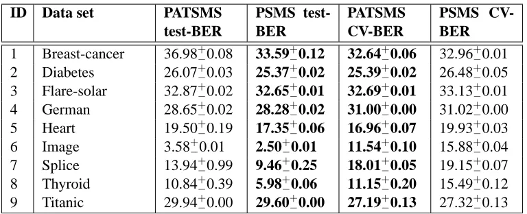
Table 4: Average and variance of test-BER and CV-BER obtained by models selected with PSMS and PATSMS, the best results are shown in bold. test-BER is the BER obtained by the selected model using the test set (averaged over 10 replications of each data set). CV-BER is the average of CV BER obtained by each of the candidate solutions through the search process (averaging performed over all particles and iterations and over 10 replications of each data set) .

The performance of both search strategies is similar. PSMS outperformed PATSMS through all of the data sets at the end of the search process (Columns 3 and 4 in Table 4). The test-BER differences are statistically significant for all but the flare-solar and german data sets. In the latter data sets the hypothesis that models selected with PATSMS and PSMS perform equally cannot be rejected. However, note that for these data sets the models selected with PSMS outperformed those selected with PATSMS in 6 out of 10 replications. Globally, we noticed that from the 90 trials (9−data sets,×10−replications for each, see Table 3), 68.9% of the models selected with PSMS outperformed those obtained with PATSMS. While only in 22.2% of the runs PATSMS outperformed PSMS, in the rest both methods tied in performance. A statistical test over these 90 results was performed and a statistically-significant difference, favoring PSMS, was found. Despite PATSMS being a strong baseline, these results give evidence that PSMS outperforms PATSMS at the end of the search process.

10 20 30 40 50 10

15 20 25 30 35 40

Iterations

BER

CV−BER

PATSMS PSMS

10 20 30 40 50 10

15 20 25 30 35 40 45 50

Iterations

BER

Test−BER

PATSMS PSMS

Figure 1: Performance of PATSMS (circles) and PSMS (triangles) as a function of number of iter-ations for an experiment with one replication of the Heart data set. For PSMS we show the performance of each particle with a different color. Left: Cross-validation Balanced Error Rate (BER). Right: Test set BER. In both plots we indicate with an arrow the model selected by each search strategy.

In Figure 1 we show the performance of the solutions tried through the search by each method for a single replication of the Heart data set (for clarity in the plots we used m=5 and I=50 for this experiment). We show the CV and test BER for every model tried through the search. It can be seen that the CV-BER of PATSMS is lower than that of PSMS, showing an apparent better convergence behavior (left plot in Figure 1). However, by looking the test BER of the models tried, it becomes evident that PATSMS is trapped into a local minimum since the very first iterations (right plot in Figure 1). PSMS, on the other hand, obtains a higher CV-BER through the search, though it is less prone to follow a local minimum. This is because with PSMS the search is guided by one global and m local solutions, which prevents PSMS from performing a pure local search; the latter in turn prevents PSMS of overfitting the data. This result gives evidence of the better convergence behavior of PSMS.

The model selected with PSMS obtained a lower test-BER than that selected with PATSMS (see right plot in Figure 1). In fact all of the solutions in the final swarm outperformed the solution obtained with PATSMS in test-BER. With PSMS the model of lowest test BER was obtained after 3 iterations of PSMS, giving evidence of the fast convergence of PSO. One should note that the test-BER of the worst PSMS solutions is higher than that of the best PATSMS solution. However, near the end of the search, the possibilities that PSMS can select a worse solution than PATSMS are small.

Figure 2: Normalized frequency of classifiers (left), feature selection method (middle) and combi-nation of preprocessing methods (right) preferred by PSMS through the search process. In the right plot, the abbreviations shift, stand and norm stand for shift-scale, standard-ization and normalstandard-ization, respectively. Results are normalized over the 90,900 models tried for obtaining the results from Table 4.

normalized frequency of methods preferred by PSMS6through the search. The results shown in this figure are normalized over the 90,900 models tried for obtaining the results from Table 4. From this figure, we can see that most of the classifiers and feature selection methods were considered for creating solutions. No classifier, feature selection method or combination of preprocessing methods was used for more than 27% of the models. This reflects the fact that different methods are required for different data sets and that some are equivalent. There were, however, some methods that were slightly more used than others.

The preferred classifier was the zarbi CLOP-object, that was used for about 23% of the models. This is a surprising result because zarbi is a very simple linear classifier that separates the classes by using information from the mean and variance of training examples (Golub et al., 1999). How-ever, in 97.35% of the times that zarbi was used it was combined with a feature selection method. Gkridge, svc, neural and logitboost were all equally selected after zarbi. Ftest was the most used feature selection method, though most of the feature selection strategies were used. Note that Pear-son, Zfilter, gs and s2n were considered only for a small number of models. The combination standardize + shift-scale was mostly used for preprocessing, although the combination normalize + standardize + shift-scale was also highly used. Interestingly, in 70.1% of the time preprocessing was performed before feature selection. These plots illustrate the diversity of classifiers considered by PSMS through the search process, showing that PSMS is not biased towards models that tend to perform very well individually (e.g., logitboost, rf or gkridge). Instead, PSMS attempts to find the best full model for each data set.

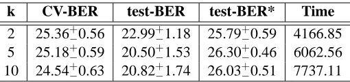
k CV-BER test-BER test-BER* Time 2 25.36+₋0.56 22.99+₋1.18 25.79+₋0.59 4166.85 5 25.18+₋0.59 20.50+₋1.53 26.30+₋0.46 6062.56 10 24.54+₋0.63 20.82+₋1.74 26.03+₋0.51 7737.11

Table 5: Average CV-BER (average CV result over all particles and iterations), test-BER (test result corresponding to the best CV result), test-BER* (average test result over all particles and iterations) and processing time (in seconds) for different values of k in the k−fold CV. Results are averaged over a single replication of each data set described in Table 3.

4.2 Parameter Selection for PSMS

In this section we analyze the performance of PSMS under different settings. The goal is to identify mechanisms in PSMS that allow us obtaining competitive models and, to some extent, avoiding overfitting. For the experiments described in this section we consider a single replication for each data set. As before, we show the average CV error of the solutions considered during the search as well as the error of the selected model in the test set. We also show the average test set error of all solutions tried through the search test-BER∗ (averaging performed over all particles and all iterations), providing information about the generalization performance of the models considered throughout the search.

4.2.1 VALUE OF K IN K-FOLDCV

First we analyze the behavior of PSMS for different values of k in the CV for computing the fitness function. We consider the values k= [2,5,10]. Average results of this experiment are shown in Table 5.

From this table, we can see that the performance is similar for the different values of k consid-ered. The best results at the end of the search are obtained with k=5 (column 3 in Table 5), while the best generalization performance is obtained with k=2 (column 4 in Table 5). However, these differences are not statistically significant. Therefore, the null hypothesis that models selected with k= [2,5,10]perform equally in test-BER and test-BER* cannot be rejected. The latter is an impor-tant result because by using k=2 the processing time of PSMS is considerably reduced. Note that for models of quadratic (or higher order) complexity, computing the fitness function with 2−fold CV is even more efficient than computing the fitness function using the full training set. It is not sur-prising that processing time increases as we increase k (column 5 in Table 5). Although it is worth mentioning that the variance in processing time was very large (e.g., for k=2 it took 7 minutes applying PSMS to the titanic data set and about five hours for the image data set).

4.2.2 NUMBERIOFITERATIONS

Setting CV-BER test-BER test-BER* I=10 25.33+₋0.33 22.17+₋1.81 27.64+₋0.52 I=25 25.29+₋0.33 21.88+₋1.68 27.59+₋0.49 I=50 24.02+₋0.38 21.12+₋1.74 26.72+₋0.65 I=100 24.57+₋0.37 22.81+₋1.44 27.27+₋0.48

m=5 24.27+₋0.49 20.81+₋1.50 25.01+₋0.85 m=10 25.07+₋0.34 21.64+₋2.04 25.99+₋0.74 m=20 25.09+₋0.34 21.76+₋1.84 26.00+₋0.64 m=40 24.82+₋0.43 21.45+₋2.13 25.96+₋0.78 m=50 25.32+₋0.44 22.54+₋1.65 26.11+₋0.77

W=(0,0,0) 23.86+₋0.71 20.40+₋1.71 22.46+₋1.32 W=(1.2,0.5,0.5) 24.22+₋0.76 19.41+₋1.37 23.38+₋1.34 W=(1,1,1) 27.62+₋0.30 21.88+₋1.68 27.13+₋0.53

Table 6: Average CV-BER, test-BER and test-BER* for different settings of m, I and W. The best results are shown in bold. Results are averaged over a single replication of each data set described in Table 3.

was not statistically significant. The difference in performance between models selected after 50 and 100 iterations was statistically significant. This result shows the fast convergence property of PSMS and that early stopping could be an useful mechanism to avoid overfitting, see Section 5.

4.2.3 SWARMSIZE M

In the next experiment we fixed the number of iterations to I=50 and varied the swarm size as fol-lows, m= [5,10,20,40,50]. Results of this experiment are shown in rows 6-10 in Table 6. This time the best result was obtained by using a swarm size of 5, however there is a statistically-significant difference only between m=5 and m=50. Therefore, models of comparable performance can be obtained by using m= [5,10,20,40]. This is another interesting result because using a small swarm size reduces the number of fitness function evaluations for PSMS and therefore makes it more prac-tical. An interesting result is that by using 50 iterations with any swarm size the test-BER is very close to the CV-BER estimate. Again, this provides evidence that early stopping can improve the average generalization performance of the models.

4.2.4 INERTIAWEIGHTW

We also performed experiments with different configurations for W, the adaptive inertia weight. Each configuration is defined by a triplet W= (wstart,wf,wend), whose elements indicate the starting

Figure 3: Algorithm performance as a function of number of iterations for different configurations of W. CV-BER (circles) and test-BER* (crosses) for the Heart data set. We are display-ing the test and CV BER values for each particle at every time step. Since each time step involves m=5 particles, then for each iteration are displayed m=5 crosses and m=5 cir-cles. We consider the following configurations: W= (0,0,0)(left), W= (1.2,0.5,0.4) (middle) and W= (1,0,1)(right). The CV-BER and test-BER of the best solution found by PSMS are enclosed within a bold circle.

The best result at the end of the search (column 3 in Table 6) was obtained with W= (1.2,0.5,0.4), the difference with the other results is statistically-significant. Under this configuration both global and local search is performed during the PSMS iterations; which caused higher CV-BER and test-BER∗than that of the first configuration, however, the generalization performance of the final model was better. The configuration W= (1,0,1)obtained the worst results in all of the measures; this is because under this configuration the search is never refined, since PSMS always takes into account the past velocity for updating solutions. The latter configuration could be a better choice for FMS because this way PSMS does not over-search around any solution; however, local search is also an important component of any search algorithm. In Figure 3 we show the CV and test BER of solutions tried during the search for the Heart data set under the different configurations tried. From this figure we can appreciate the fact that using constant values for W results in more local (when W= (0,0,0)) or global search (when W= (1,0,1)). An adaptive inertia weight, on the other hand, aims to control the tradeoff between global and local search, which results in a model with lower variance for this example. Therefore, an adaptive inertia weight seems to be a better option for FMS; this is because it prevents, to some extend, PSMS to overfit the data. However, further experiments need to be performed in order to select the best configuration for W.

4.2.5 INDIVIDUAL(c1) ANDGLOBAL(c2) WEIGHTS

We now analyze the performance of PSMS under different settings of the individual (c1) and global

(c2) weights. We considered three configurations for c1and c2; in the first one both weights have the

same influence in the search (i.e., c1=2; c2=2), this was the setting used for all of the experiments

reported in Section 4. In the second setting the local weight has no influence in the search (i.e., c1=0; c2=2), while in the third configuration the global weight is not considered in the search

ID Setting CV-BER test-BER test-BER* 1 c1=2; c2=2 23.69−+0.68 19.72+−1.45 23.92+−1.16

2 c1=0; c2=2 26.87−+0.43 22.42+−1.32 27.13+−0.55

3 c1=2; c2=0 24.99−+0.41 21.73+−1.42 25.59+−0.66

Table 7: Average CV-BER, test-BER and test-BER* for different settings of c1 and c2in Equation

(1). The best results are shown in bold. Results are averaged over a single replication of each data set described in Table 3.

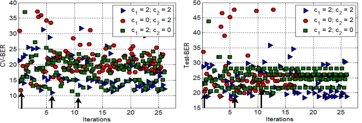
Figure 4: Performance of PSMS as a function of number of iterations using different settings for c1 and c2, see Table 7. We show the CV-BER (left) and Test-BER (right) for a single

replication of the Heart data set. PSMS was ran for I=25 iterations in this experiment. The models selected with each configuration are indicated with arrows.

replication for each data set described in Table 3; for the three configurations considered it was used the same adaptive inertia weight W= (1.2,0.5,0.4); averaged results of this experiment are shown in Table 7.

From this table we can see that the best performance is obtained by assigning equal weights to both factors. The difference in performance is statistically-significant over all measures with respect to the other two configurations. Therefore, by using the first configuration we can obtain solutions of better performance through and at the end of the search. More importantly, solutions of better generalization performance can be obtained with this configuration as well. The difference in performance is higher with the second configuration, where the individual-best solutions have no influence in the search; therefore, PSMS is searching locally around the global best solution. In the third configuration the global-best solution has no influence in the search; in consequence, the search is guided according the m−individual-best solutions. For illustration in Figures 4 and 5 we show the performance of PSMS as a function of the number of iterations for a single replication of the Heart data set. In Figure 4 we show the performance of PSMS for I=25 iterations and in Figure 5 for I=100 iterations.

Figure 5: Performance of PSMS as a function of number of iterations using different settings for c1 and c2, see Table 7. We show the CV-BER (left) and Test-BER (right) for a single

replication of the Heart data set. PSMS was ran for I=100 iterations in this experiment. The models selected with each configuration are indicated with arrows.

the data (red circles and green squares). With c1=0 we have that the m=5 particles converge to

single local minima, performing a fine grained search over this solution (red circles). With c2=0

each of the m−particles converge to different local minima, overdoing the search over each of the m solutions (green squares). On the other hand, with the configuration c1=2, c2=2 PSMS is not

trapped into a local minimum (blue triangles); searching around promising solutions, but without doing a fine grained search over any of them.

Better models (indicated by arrows) are selected by PSMS with the first configuration, even when their CV is higher than that of the models selected with the other configurations. This result confirms that PSMS is overfitting the data with the configurations 2 and 3. Note that with I=25 iterations (Figure 4) the first configuration is not converging to a local minimum yet; while with I=100 iterations (Figure 5) it looks like PSMS starts searching locally at the last iterations. This result illustrates why early stopping can be useful for obtaining better models with PSMS.

In order to better appreciate the generalization performance for the different configurations, in Figure 6 we plot the CV-BER as a function of test-BER for the run of PSMS with I=25, we plot each particle with a different color.

From this figure we can see that the best model is obtained with the first configuration; for the configurations 2 and 3 the particles obtain the same test-BER for different solutions (middle and right plots in Figure 6). Despite the CV estimate is being minimized for these configurations, the test-BER performance of models does not improve. It is clear from the right plot in Figure 6 that with c2=0 each particle is trapped in different local minima, doing a fine grained search over them

that causes PSMS to overfit the data. It also can be seen from the middle plot that with c1=0

the search is biased towards a single global-best solution (magenta circle), again, causing PSMS to overfit the data. On the other hand, results with the first configuration (left plot in Figure 6) show that particles do not oversearch at any solution.

4.3 Results on the Model Selection Challenge

Figure 6: Test-BER as a function of CV-BER for a run of PSMS for I=25 iterations in the Heart data set. Results with different configurations for c1 and c2 are shown. Left: c1=2,

c2=2. Middle: c1=0, c2=2. Right: c1=2, c2=0. In each plot each particle is shown

with a different color. The selected model with each configuration is indicated with an arrow.

2008). The goal of these experiments is to compare the performance of PSMS against other model selection strategies that work for a single algorithm or that use domain knowledge for this task. Through its different stages, the ALvsPK competition evaluated novel strategies for model selection as well as the added value of using prior knowledge for improving classification accuracy (Guyon et al., 2008). This sort of competitions are very useful because through them the real effectiveness of methods can be evaluated; motivating further research in the field and collaborations among participants.

4.3.1 CHALLENGEPROTOCOL AND CLOP

The rules of the challenge were quite simple, the organizers provided five data sets for binary clas-sification together with the CLOP toolbox (Saffari and Guyon, 2006). The task was to obtain the model with the lowest BER over the five data sets on unseen data. Participants were free to elect using CLOP or their own learning machine implementations. The challenge is over now, although the challenge website7still remains open, allowing the evaluation of learning techniques and model selection methods. A complete description of the challenge and a comprehensive analysis of the results are described by Guyon et al. (2006c, 2007, 2008).

The competition was divided into two stages. The first stage, called the model selection game (Guyon et al., 2006c), was focused on the evaluation of pure model selection strategies. In the sec-ond stage, the goal was to evaluate the gain we can have by introducing prior knowledge into the model selection process (Guyon et al., 2007, 2008). In the latter stage participants could introduce knowledge of the data domain into the model selection process (prior knowledge track). Also, par-ticipants could use agnostic methods in which no domain knowledge is considered in the selection process (agnostic track).

The data sets used in the agnostic track of the ALvsPK challenge are described in Table 8, these data sets come from real domains. Data sets used for the agnostic and prior knowledge tracks were

different. For the agnostic track the data were preprocessed and dummy features were introduced, while for the prior knowledge track raw data were used, together with a description of the domain. We should emphasize that, although all of the approaches evaluated in the ALvsPK competition faced the same problem (that of choosing a model that obtains the lowest classification error for the data), such methods did not adopt the FMS interpretation. Most of the proposed approaches focused on a fixed machine learning technique like tree-based classifiers (Lutz, 2006), or kernel-based methods (Cawley, 2006; Pranckeviciene et al., 2007; Guyon et al., 2008), and did not take into account feature selection methods. Participants in the prior knowledge track could introduce domain knowledge. Furthermore, most of participants used their own implementations, instead of the CLOP toolbox.

After the challenge, the CLOP toolkit was augmented with methods, which performed well in the challenge (Cawley, 2006; Cawley and Talbot, 2007a; Lutz, 2006). These include Logit-boost (Friedman et al., 2000), LSSVM (Suykens and Vandewalle, 1999), and kernel ridge regres-sion (Saunders et al., 1998; Hastie et al., 2001).

4.3.2 COMPETITIVENESS OF PSMS

In both stages of the competition we evaluated models obtained with PSMS under different settings. Models obtained by PSMS were ranked high in the participants list, showing the competitiveness of PSMS for model selection (Guyon et al., 2006c, 2007, 2008; Escalante et al., 2007). Furthermore, the difference with methods that used prior knowledge was relatively small, showing that FMS can be a viable solution for the model selection problem without the need of investing time in introducing domain knowledge, and by considering a wide variety of methods.

The results of PSMS in the ALvsPK challenge have been partially analyzed and discussed else-where (Escalante et al., 2007; Guyon et al., 2007, 2008). During the challenge, our best entry (called Corrida-final) was ranked88thover all ranked participants, 5thamong the methods that did not use domain knowledge and 2nd among the methods that used the software provided by the organizers (Guyon et al., 2006c, 2007, 2008). For Corrida-final we used k=5 and the full training set for com-puting the fitness function; we ran PSMS for 500 iterations for the Ada data set and 100 iterations for Hiva, Gina and Sylva. We did not applied PSMS to the Nova data set in that entry, instead we selected a model for Nova by trial and error. For such entry we used a version of CLOP where only there were available the following classifiers zarbi, naive, neural and svc (Escalante et al., 2007); also, only four feature selection methods were considered.

4.3.3 POST-CHALLENGEEXPERIMENTS

In the rest of this section we present results of PSMS using the augmented toolkit, including all methods described in Tables 1 and 2. In these tables we consider implementations of logitboost, lssvm and gkridge, which are the classifiers that won the ALvsPK challenge (Cawley, 2006; Cawley and Talbot, 2007a; Lutz, 2006) and were added to CLOP after the end of the challenge.

In order to efficiently apply PSMS to the challenge data sets we adopted a subsample strategy in which, instead of using the full training set, small subsamples of the training data were used to compute the fitness function. Each time the fitness function is computed we obtain a different random sample of size Ssub= _SFN, where N is the number of instances and SF is a constant that

specifies the proportion of samples to be used. Subsamples are only used for the search process. At

Data set Domain Type Features Training Validation Testing

Ada Marketing Dense 48 4174 415 41471

Gina Digits Dense 970 3153 315 31532

Hiva Drug discovery Dense 1617 3845 384 38449

Nova Text classification Sparse binary 16969 1754 175 17537

Sylva Ecology Dense 216 13086 1309 130857

Table 8: Benchmark data sets used for the model selection challenges (Guyon et al., 2006c, 2007, 2008).

Data SF Model Time (m) Test-BER

Ada 1 chain({logitboost(units=469,shrinkage=0.4,depth=1),bias} 368.12 16.86

Gina 2 chain({sns(1),relief(fmax=487),gkridge,bias} 482.23 2.41

Hiva 3 chain({norm(1),rffs(fmax=1001),lssvm(gamma=0.096),bias} 124.54 28.01

Nova 1 chain({rffs(fmax=338),norm(1),std(1),sns(1),gkridge,bias} 82.12 5.27

Sylva 10 chain({sns(1),odds-ratio(fmax=60),gkridge,bias} 787.58 0.62

Table 9: Models selected with PSMS for the data sets of the ALvsPK challenge. For each data set we show the subsampling factor used (SF), the selected model (Model, some hyperparameters are omitted for clarity), the processing Time in minutes and the test-BER obtained. sns is for shit-scale, std is for standardize and norm is for normalize. See Tables 1 and 2 for a description of methods and their hyperparameters.

the end of the search the selected model is trained using the full training set (for the experiments reported in this paper we considered as training set the union of the training and validation data sets, see Table 8). Due to the dimensionality of the Nova data set we applied principal component analysis to this data set. Then we used the first 400 components for applying PSMS. We fixed k=2, I =50 and m=5 for our experiments based on the results from previous sections. Then we ran PSMS for all of the data sets under the above described settings using different values for SF. The predictions of the resultant models were uploaded to the challenge website in order to evaluate them. Our best ranked entry in the ALvsPK challenge website (called psmsx jmlr run I) is described in Table 9, and a comparison of it with the currently best-ranked entries is shown in Table 10.