Learnability, Stability and Uniform Convergence

Learnability, Stability and Uniform Convergence

Shai Shalev-Shwartz [email protected]

School of Computer Science and Engineering The Hebrew University of Jerusalem Givat Ram, Jerusalem 91904, Israel

Ohad Shamir [email protected]

Microsoft Research One Memorial Drive Cambridge, MA 02142, USA

Nathan Srebro [email protected]

Karthik Sridharan [email protected]

Toyota Technological Institute at Chicago 6045 S. Kenwood Ave.

Chicago, IL 60637, USA

Editor: Nicol`o Cesa-Bianchi

Abstract

The problem of characterizing learnability is the most basic question of statistical learning theory. A fun-damental and long-standing answer, at least for the case of supervised classification and regression, is that learnability is equivalent to uniform convergence of the empirical risk to the population risk, and that if a problem is learnable, it is learnable via empirical risk minimization. In this paper, we consider the General Learning Setting (introduced by Vapnik), which includes most statistical learning problems as special cases. We show that in this setting, there are non-trivial learning problems where uniform convergence does not hold, empirical risk minimization fails, and yet they are learnable using alternative mechanisms. Instead of uniform convergence, we identify stability as the key necessary and sufficient condition for learnability. More-over, we show that the conditions for learnability in the general setting are significantly more complex than in supervised classification and regression.

Keywords: statistical learning theory, learnability, uniform convergence, stability, stochastic convex opti-mization

1. Introduction

We consider the General Setting of Learning introduced by Vapnik (1995) where we would like to minimize a population risk functional (stochastic objective)

F(h) =EZ∼D[f(h; Z)] (1)

over some hypothesis class

H

, where the distribution

D

of Z is unknown, based on i.i.d. sample z1, . . . ,zm

drawn from

D

(and full knowledge of f and

H

). This General Setting subsumes supervised classification and regression, certain unsupervised learning problems, density estimation and more. For example, in super-vised learning z= (x,y)is an instance-label pair, h is a predictor, and f(h;(x,y)) =loss(h(x),y)is the loss functional. See Section 2 for formal definitions and further examples.

In the context of this general setting, we are concerned with the question of statistical “learnability”. That is, when can Equation (1) be minimized to within arbitrary precision based only on a finite sample z1, . . . ,zm,

For supervised classification and regression problems, it is well known that a problem is learnable if and only if the empirical risks

FS(h) =_m1 m

∑

i=1

f(h,zi)

for all h_∈

H

converge uniformly to the population risk (Blumer et al., 1989; Alon et al., 1997). If uniform convergence holds, then the empirical risk minimizer (ERM) is consistent, that is, the population risk of the ERM converges to the optimal population risk, and the problem is learnable using the ERM. We therefore have:

• A necessary and sufficient condition for learnability, namely uniform convergence of the empirical risks. Furthermore, this can be shown to be equivalent to a combinatorial condition: having finite VC-dimension in the case of classification, and having finite fat-shattering dimensions in the case of regression.

• A complete understanding of how to learn: since learnability is equivalent to learnability by ERM, we can focus our attention solely on empirical risk minimizers.

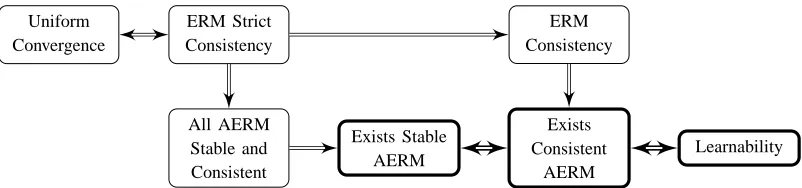
The situation, for supervised classification and regression, can be depicted as follows:

Finite Dim. Uniform Convergence

Learnable

with ERM Learnable

Other than uniform convergence, certain notions of stability have also been suggested as an explicit condition for learnability. Intuitively, stability notions focus on particular algorithms, or learning rules, and measure their sensitivity to perturbations in the training set. In particular, it is known that stability of the ERM is sufficient for learnability. In Mukherjee et al. (2006), it is argued that stability is also a necessary for learnability. However, that argument relied on the assumption that uniform convergence is equivalent to learnability. Therefore, stability was shown to characterize learnability only in situations where uniform convergence characterizes learnability anyway.

The equivalence of uniform convergence and learnability was formally established only in the supervised classification and regression setting. In the more general setting, the “rightward” implications in the diagram above still hold: finite fat-shattering dimensions, uniform convergence, as well as ERM stability, are indeed sufficient conditions for learnability using the ERM. As for the reverse implication, Vapnik showed that a notion of “non-trivial” or “strict” learnability with the ERM is indeed equivalent to uniform convergence of the empirical risks. This notion was meant to exclude certain “trivial” learning problems, which are learn-able without uniform convergence (see Section 3.1). Even in such problems, learnability is still possible by empirical risk minimization. Thus, it would seem that in the General Learning Setting, as in supervised clas-sification and regression, a problem is learnable if and only if it is learnable by empirical risk minimization.

In this paper we show that the situation in the General Learning Setting is actually much more complex. In particular, in Section 4.1 we show an example of a learning problem in the General Learning Setting, which is learnable (using an online algorithm and an online-to-batch conversion), but which is not learnable using empirical risk minimization. To the best of our knowledge this is the first example shown of this type.

Furthermore, in Section 4.2 we show a modified example which is learnable using empirical risk mini-mization, but for which the empirical risks of the hypotheses do not converge uniformly to their expectations, not even locally for hypotheses very close to the true hypothesis. We argue that unlike the examples discussed in Section 3.1, this example is far from being “trivial”. We use this example to discuss how Vapnik’s notion of “strict” learnability with the ERM is too strict, and precludes cases which are far from trivial and in which learnability with empirical risk minimization is not equivalent to uniform convergence.

In particular, we show that for learnable problems, even when they are not learnable with ERM, they are always learnable with some learning rule which is “asymptotically ERM” and (AERM - see precise definition in Section 2). Moreover, such an AERM must be stable (under a suitable notion of stability). Namely, we have the following characterization of learnability in the General Learning Setting:

Exists Stable AERM

Learnable

with AERM Learnable

Note that this characterization holds even for learnable problems with no uniform convergence. In this sense, stability emerges as a strictly more powerful notion than uniform convergence for characterizing learnability. Other than this, we also discuss several related results, which above all imply that the conditions for learnability in the General Learning Setting are substantially different and more complex than in supervised classification and regression.

Our results point not to a specific learning rule (such as an ERM), but rather to a class of learning rules (AERM learning rules) as possible candidates for learning. In Section 6, we explore how our results can be strengthened if we allow randomized learning rules. In particular, randomization allows us to pinpoint not a general class of learning rules, but rather a specific (though highly impractical) learning rule, which learns if and only if the problem is learnable.

Throughout most of the paper we discuss learning rates (as a function of the sample size), but do not pay much attention to the confidence at which the learning rule succeeds (i.e., the dependence of the sample size on the allowed probability of failure). This issue is addressed Section 7, and again we show that in the General Learning Setting, things can behave rather differently than in supervised classification and regression.

In summary, this paper opens a door to the complexity of learnability in the General Learning Setting, and provides some understanding of the situation, including highlighting the important role of stability. Many gaps in our understanding remain, and we hope that future progress will close some of these gaps, as well as connect the theoretical insights gained to machine learning as used in practice.

This paper is partially based on the results obtained in Shalev-Shwartz et al. (2009a) and Shalev-Shwartz et al. (2009b).

2. The General Learning Setting: Formal Definition and Notation

In this paper we focus on the General Learning Setting, which was introduced by Vapnik (1995) as a unifying framework for the problem of statistical learning from empirical data.

The General Learning Setting deals with learning problems. Formally, a learning problem is specified by a hypothesis class

H

, an instance set

Z

(with a sigma-algebra), and an objective function (e.g., “loss” or “cost”) f :

H

×

Z

→R. Throughout this paper we assume the function is bounded by some constant B, that is_|f(h; z)| ≤B for all h_∈

H

and z_∈

Z

.

Given a distribution

D

on

Z

, the quality of each hypothesis h_∈

H

is measured by its risk F(h), which is defined asEz_∼D[f(h; z)]. While

H

,

Z

and f(h; z)are known to the learner, we assume that

D

is unknown.

Ideally, we would like to pick h_∈

H

whose risk is as close as possible to inf_h∈HF(h). Since the underlying distribution

D

is unknown, we cannot do this directly, but instead need to rely on a finite empirical training

sample S={z1, . . . ,zm}. On this sample, we apply a learning rule to pick a hypothesis . Formally, a learning

rule is a mapping A :_∪∞_m=1

Z

m_→

_H

_{from sequences of instances in}

_Z

_{to hypotheses. We refer to sequences} S={z1, . . . ,zm}as “sample sets”, but it is important to remember that the order and multiplicity of instances

may be significant. A learning rule that does not depend on the order of the instances in the training sample is said to be symmetric. We will generally consider samples S_∼

D

m_{of m i.i.d. draws from}

_D

_.

• Binary Classification: Let

Z

=

X

× {0,1}, let

H

be a set of functions h :

X

7→ {0,1_}, and let

f(h;(x,y)) = 11_{h(x)6=y}. Here, f(·)is simply the 0₋1 loss function, measuring whether the binary hypothesis h(·)misclassified the example(x,y).

• Regression: Let

Z

=

X

×

Y

where

X

and

Y

are bounded subsets ofRnandRrespectively, let

H

be a set of bounded functions h :

X

n_{7→R, and let f(h;(x,y)) = (h(x)−y)}2_{. Here, f(·)is simply the} squared loss function.

• Large Margin Classification in a Reproducing Kernel Hilbert Space (RKHS): Let

Z

=

X

_{× {}0,1}, where

X

is a bounded subset of an RKHS, let

H

be another bounded subset of the RKHS, and let

f(h;(x,y)) =max_{0,1₋y_hx,h_i}. Here, f(·)is the well known hinge loss function, and our goal is to perform margin-based linear classification in the RKHS.

• K-Means Clustering in Euclidean Space: Let

Z

=Rn, let

H

be all subsets ofRnof size k, and let

f(h; z) =minc∈hkc−zk2. Here, each h represents a set of k centroids, and f(·)measures the Euclidean

distance squared between an instance z and its nearest centroid, according to the hypothesis h.

• Density Estimation: Let

Z

be a subset ofRn, let

H

be a set of bounded probability densities on

Z

, and let f(h; z) =−log(h(z)). Here, f(·)is simply the negative log-likelihood of an instance z according to the hypothesis density h. Note that to ensure boundedness of f(·), we need to assume that h(z)is lower bounded by a positive constant for all z_∈

Z

.

• Stochastic Convex Optimization in Hilbert Spaces: Let

Z

be an arbitrary measurable set, let

H

be a closed, convex and bounded subset of a Hilbert space, and let f(h; z)be Lipschitz-continuous and convex w.r.t. its first argument. Here, we want to approximately minimize the objective function

Ez∼D[f(h; z)], where the distribution over

Z

is unknown, based on an empirical sample z1, . . . ,zm.

Our overall goal in this setting is to pick a hypothesis h_∈

H

with approximately minimal possible risk, based on a finite sample. Generally, we expect the approximation to get better with the sample size. Learning rules which allow us to choose such hypotheses are said to be consistent. Formally, we say a rule A is consistent with rateεcons(m)under distribution

D

if for all m,

ES_∼Dm[F(A(S))−F∗]≤ε_cons(m), (2)

where we denote F∗=inf_h∈HF(h)(here and whenever talking about a “rate” ε(m), we require it to be monotone decreasing withεcons(m)

m_→∞

−→0).

However, since

D

is unknown, we cannot choose a learning rule based on

D

. Instead, we will ask for a stronger requirement, namely that the rule is consistent with rateεcons(m)under all distributions

D

over

Z

. This leads to the following central definition:

Definition 1 A learning problem is learnable, if there exist a learning rule A and a monotonically decreasing

sequenceεcons(m), such thatεcons(m)

m→∞

−→0, and

∀

D

, ES_∼Dm[F(A(S))−F∗]≤ε_cons(m).

A learning rule A for which this holds is denoted as a universally consistent learning rule.

This definition of learnability, requiring a uniform rate for all distributions, is the relevant notion for studying learnability of a hypothesis class. It is a direct generalization of agnostic PAC-learnability (Kearns et al., 1992) to Vapnik”s General Setting of Learning as studied by Haussler (1992) and others.

A possible approach to learning is to minimize the empirical risk FS(h)over a sample S, defined as

FS(h) =

1

Z

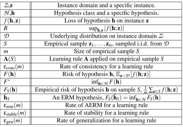
,z Instance domain and a specific instance.

H

,h Hypothesis class and a specific hypothesis.

f(h,z) Loss of hypothesis h on instance z

B sup_h,z|f(h; z)|

D

Underlying distribution on instance domain

Z

S Empirical sample z1, . . . ,zm, sampled i.i.d. from

D

m Size of empirical sample S

A(S) Learning rule A applied on empirical sample S

εcons(m) Rate of consistency for a learning rule

F(h) Risk of hypothesis h,Ez∼D[f(h; z)]

F∗ inf_h∈H F(h)

FS(h) Empirical risk of hypothesis h on sample S, _m1∑z_∈Sf(h; z)

ˆhS An ERM hypothesis, FS(ˆhS) =infh∈HFS(h) εerm(m) Rate of AERM for a learning rule

εstable(m) Rate of stability for a learning rule

εgen(m) Rate of generalization for a learning rule

Table 1: Table of Notation

We say that a rule A is an ERM (Empirical Risk Minimizer) if it minimizes the empirical risk

FS(A(S)) =FS(ˆhS) = inf h∈HFS(h).

where we use FS(ˆhS) =infh∈H FS(h)to refer to the minimal empirical risk. But since there might be several

hypotheses minimizing the empirical risk, ˆhSdoes not refer to a specific hypotheses and there might be many

rules which are all ERM.

We say that a rule A is an AERM (Asymptotic Empirical Risk Minimizer) with rateεerm(m)under distri-bution

D

if:

ES∼DmF_S(A(S))−F_S(ˆh_S)≤ε_erm(m)

A learning rule is universally an AERM with rate εerm(m), if it is an AERM with rateεerm(m) under all distributions

D

over

Z

. A learning rule is an always AERM with rateεerm(m), if for any sample S of size m, it holds that FS(A(S))−FS(ˆhS)≤εerm(m).

We say a rule A generalizes with rateεgen(m)under distribution

D

if for all m,

ES∼Dm[|F(A(S))−F_S(A(S))|]≤ε_gen(m).

A rule universally generalizes with rateεgen(m)if it generalizes with rateεgen(m)under all distributions

D

over

Z

.

We note that other authors sometimes define “consistent”, and thus also “learnable” as a combination of our notions of “consistent” and “generalizing”.

In the above definitions, we choose to use convergence in expectation, and defined the rates as rates on the expectation. Since the objective f is bounded, convergence in expectation is equivalent to convergence in probability. Furthermore, using Markov’s inequality we can translate a rate of the formE[|X|]≤ε(m)to a “low confidence” guaranteeP[|X_|>ε(m)/δ]≤δ. See Section 7 for a further discussion on this issue.

3. Background: Characterization of Learnability

3.1 Learnability and Uniform Convergence

As discussed in the introduction, a central notion for characterizing learnability is uniform convergence. Formally, we say that uniform convergence holds for a learning problem, if the empirical risks of hypotheses in the hypothesis class converges to their population risk uniformly, with a distribution-independent rate:

sup

D ES∼D

m

"

sup

h∈H|

F(h)−FS(h)| #

m→∞

−→0.

It is straightforward to show that if uniform convergence holds, then a problem can be learned with the ERM learning rule.

For binary classification problems (where

Z

=

X

×{0,1_}, each hypothesis is a mapping from

X

to_{0,1}, and f(h;(x,y)) = 11_{h(x)6=y_}), Vapnik and Chervonenkis (1971) showed that the finiteness of a simple

com-binatorial measure known as the VC-dimension implies uniform convergence. Furthermore, it can be shown that binary classification problems with infinite VC-dimension are not learnable in a distribution-independent sense. This establishes the condition of having finite VC-dimension, and thus also uniform convergence, as a necessary and sufficient condition for learnability.

Such a characterization can also be extended to regression, such as regression with squared loss, where h is now a real-valued function, and f(h;(x,y)) = (h(x)−y)2_{. The property of having finite fat-shattering} dimension at all finite scales now replaces the property of having finite VC-dimension, but the basic equiva-lence still holds: a problem is learnable if and only if uniform convergence holds (Alon et al., 1997, see also Anthony and Bartlet, 1999, Chapter 19). These results are usually based on clever reductions to binary clas-sification. However, the General Learning Setting that we consider is much more general than classification and regression, and includes setting where a reduction to binary classification is impossible.

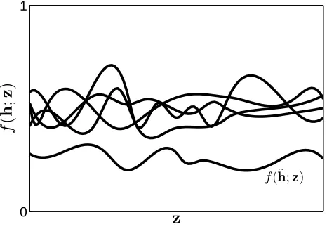
To justify the necessity of uniform convergence even in the General Learning Setting, Vapnik attempted to show that in this setting, learnability with the ERM learning rule is equivalent to uniform convergence (Vapnik, 1998). Vapnik noted that this result does not hold, due to “trivial” situations. In particular, consider the case where we take an arbitrary learning problem (with hypothesis class

H

), and add to

H

a single hypothesis ˜h such that f(˜h,z)<inf_h∈H f(h,z)for all z_∈

Z

(see figure 1 below). This learning problem is now trivially learnable, with the ERM learning rule which always picks ˜h. Note that no assumptions whatsoever are made on

H

- in particular, it can be arbitrarily complex, with no uniform convergence or any other particular property. Note also that such a phenomenon is not possible in the binary classification setting, where f(h;(x,y)) = 11_{h(x)6=y}, since on any(x,y)we will have hypotheses with f(h;(x,y)) = f(˜h;(x,y)) and thus if

H

is very complex (has infinite VC dimension) then on every training set there will be many hypotheses with zero empirical error.

To exclude such “trivial” cases, Vapnik introduced a stronger notion of consistency, termed as “strict consistency”, which in our notation is defined as

∀c_∈R, inf

h:F(h)≥c FS(h)

m_→∞

−→ inf

h:F(h)≥c F(h),

where the convergence is in probability. The intuition is that we require the empirical risk of the ERM to converge to the lowest possible risk, even after discarding all the “good” hypotheses whose risk is smaller than some threshold. Vapnik then showed that such strict consistency of the ERM is in fact equivalent to (one-sided) uniform convergence, of the form

sup

h∈H

(F(h)−FS(h))m−→→∞0

in probability. Note that this equivalence holds for every distribution separately, and does not rely on universal consistency of the ERM.

0 1

z

f

(

h

;

z

)

f(˜h;z)

Figure 1: An example of a “trivial” learning situation. Each line represents some h_∈

H

, and shows the value of f(h,z)for all z_∈

Z

. The hypothesis ˜h dominates any other hypothesis (e.g., f(˜h;z)<f(h; z) uniformly for all z), and thus the problem is learnable without uniform convergence or any other property of

H

.

3.2 Learnability and Stability

Instead of focusing on the hypothesis class, and ensuring uniform convergence of the empirical risks of hypothesis in this class, an alternative approach is to directly control the variance of the learning rule. Here, it is not the complexity of the hypothesis class which matters, but rather the way that the learning rule explores this hypothesis class. This alternative approach leads to the notion of stability in learning. It is important to note that stability is a property of a learning rule, not of the hypothesis class.

In the context of modern learning theory,1 _{the use of stability can be traced back at least to the work} of Rogers and Wagner (1978), which noted that the sensitivity of a learning algorithm with regard to small changes in the sample controls the variance of the leave-one-out estimate. The authors used this observation to obtain generalization bounds (w.r.t. the leave-one-out estimate) for the k-nearest neighbor algorithm. It is interesting to note that a uniform convergence approach for analyzing this algorithm simply cannot work, because the “hypothesis class” in this case has unbounded complexity. These results were later extended to other “local” learning algorithms (see Devroye et al., 1996 and references therein). In addition, practi-cal methods have been developed to introduce stability into learning algorithms, in particular the Bagging technique introduced by Breiman (1996).

Over the last decade, stability was studied as a generic condition for learnability. Kearns and Ron (1999) showed that an algorithm operating on a hypothesis class with finite VC dimension is also stable (under a certain definition of stability). Bousquet and Elisseeff (2002) introduced a strong notion of stability (denoted as uniform stability) and showed that it is a sufficient condition for learnability, satisfied by popular learning algorithms such as regularized linear classifiers and regressors in Hilbert spaces (including several variants of SVM). Kutin and Niyogi (2002) introduced several weaker variants of stability, and showed how they are sufficient to obtain generalization bounds for algorithms stable in their sense.

The papers above mainly considered stability as a sufficient condition for learnability. A more recent line of work (Rakhlin et al., 2005; Mukherjee et al., 2006) studied stability as a necessary condition for learnability. However, the line of argument is specific to settings where uniform convergence holds and is

necessary for learning. With this assumption, it is possible to show that the ERM algorithm is stable, and thus stability is also a necessary condition for learning. However, as we will see later on in our paper, uniform convergence is in fact not necessary for learning in the General Learning Setting, and stability plays there a key role which has nothing to do with uniform convergence.

Finally, it is important to note that the results cited above make use of many different definitions of stability, which unfortunately are not always comparable. All of them measure stability as the amount of change in the algorithm’s output as a function of small changes to the sample on which the algorithm is run. However, “amount of change to the output” and “small changes to the sample” can be defined in many different ways. “Amount of change to the output” can mean change in risk, change in loss with respect to particular examples, or supremum of change in loss over all examples. “Small changes to the sample” usually mean either deleting one example or replacing it with another one (and even here, one can talk about removing/replacing one instance at random, or in some arbitrary manner). Finally, this measure of change can be measured with respect to any arbitrary sample, in expectation over samples drawn from the underlying distribution; or in high probability over samples. For further discussion of this issue, see Appendix A.

4. Gaps Between Learnability, Uniform Convergence and ERM

In this section, we study a special case of the General Learning Setting, where there is a real gap between learnability and uniform convergence, in the sense that there are non-trivial problems where no uniform convergence holds (not even in a local sense), but they are still learnable. Moreover, some of these problems are learnable with an ERM (again, without any uniform convergence), and some are not learnable with an ERM, but rather with a different mechanism. We also discuss why this peculiar behavior does not formally contradict Vapnik’s results on the equivalence of strict consistency of the ERM and uniform convergence, as well as the important role that regularization seems to play here, but in a different way than in standard theory.

4.1 Learnability without Uniform Convergence : Stochastic Convex Optimization

A stochastic convex optimization problem is a special case of the General Learning Setting discussed above, with the added constraints that the objective function f(h; z)is Lipschitz-continuous and convex in h for every z, and that

H

is closed, convex and bounded. We will focus here on problems where

H

is a subset of a Hilbert space. A special case is the familiar linear prediction setting, where z= (x,y)is an instance-label pair, each hypothesis h belongs to a subset

H

of a Hilbert space, and f(h; x,y) =ℓ(hh,φ(x)i,y)for some feature mappingφand a loss functionℓ:R×

Y

→R, which is convex w.r.t. its first argument.

The situation in which the stochastic dependence on h is linear, as in the preceding example, is fairly well understood. When the domain

H

and the mappingφare bounded, we have uniform convergence, in the sense that_|F(h)−FS(h)|is uniformly bounded over all h∈

H

(see Sridharan et al., 2008). This uniform

convergence of FS(h)to F(h)justifies choosing the empirical minimizer ˆhS=arg minhFS(h), and guarantees

that the expected value of F(ˆhS)converges to the optimal value F∗=infhF(h).

Even if the dependence on h is not linear, it is still possible to establish uniform convergence (using covering number arguments) provided that

H

is finite dimensional. Unfortunately, when we turn to infinite dimensional hypothesis spaces, uniform convergence might not hold and the problem might not be learnable with empirical minimization. Surprisingly, it turns out that this does not imply that the problem is unlearnable. We will show that using a regularization mechanism, it is possible to devise a learning algorithm for any stochastic convex optimization problem, even when uniform convergence does not hold. This mechanism is fundamentally related to the idea of stability, and will be a good starting point for our more general treatment of stability and learnability in the next section of the paper.

We now turn to discuss our first concrete example. Consider the convex stochastic optimization problem given by

f(3)(h;(x,α)) = kα∗(h−x)k = r

∑

i

where for now we let

H

to be the d-dimensional unit sphere

H

=

h_∈Rd :_kh_{k ≤}1 , we let z= (x,α)with

α∈[0,1]d_{and x∈}

_H

_{, and we define u∗v to be an element-wise product. We will first consider a sequence of}

problems, where d=2mfor any sample size m, and establish that we cannot expect a convergence rate which is independent of the dimensionality d. We then formalize this example in infinite dimensions.

One can think of the problem in Equation (3) as that of finding the “center” of an unknown distribution over x_∈Rd_{, where we also have stochastic per-coordinate “confidence” measuresα[i]. We will actually}

focus on the case where some coordinates are missing, namely thatα[i] =0.

Consider the following distribution over(x,α): x=0 with probability one, andαis uniform over_{0,1}d_.

That is,α[i]are i.i.d. uniform Bernoulli. For a random sample(x1,α1), . . . ,(xm,αm)if d>2mthen we have

that with probability greater than 1₋e−1>0.63, there exists a coordinate j∈1. . .d such that all confidence

vectorsαi in the sample are zero on the coordinate j, that isαi[j] =0 for all i=1..m. Let ej∈

H

be the

standard basis vector corresponding to this coordinate. Then

F_S(3)(ej) =

1

m m

∑

i=1

αi∗(ej−0)

=

1

m m

∑

i=1

|αi[j]| = 0,

where F_S(3)(·)denotes the empirical risk w.r.t. the function f(3)(·). On the other hand, letting F(3)_(·)denote the actual risk w.r.t. f(3)(·), we have

F(3)(ej) = Ex,αα∗(ej−0)

= Ex,α[|α[j]|] = 1/2.

Therefore, for any m, we can construct a convex Lipschitz-continuous objective in a high enough dimension such that with probability at least 0.63 over the sample, sup_h

F

(3)_(h)−F(3) S (h)

≥1/2. Furthermore, since f(·;_·)is non-negative, we have that ejis an empirical minimizer, but its expected value F(3)(ej) =1/2 is far

from the optimal expected value minhF(3)(h) =F(3)(0) =0.

To formalize the example in a sample-size independent way, take

H

to be the unit sphere of an infinite-dimensional Hilbert space with orthonormal basis e1,e2, . . ., where for v∈

H

, we refer to its coordinates v[j] =

v,ej

w.r.t this basis. The confidencesαare now a mapping of each coordinate to[0,1]. That is, an infinite sequence of reals in[0,1]. The element-wise product operationα∗v is defined with respect to this basis and the objective function f(3)(·)of Equation (3) is well defined in this infinite-dimensional space.

We again take a distribution over z= (x,α)where x=0 andαis an infinite i.i.d. sequence of uniform Bernoulli random variables (that is, a Bernoulli process with eachαiuniform over_{0,1_}and independent of all otherαj). Now, for any finite sample there is almost surely a coordinate j withαi[j] =0 for all i, and so

we a.s. have an empirical minimizer F_S(3)(ej) =0 with F(3)(ej) =1/2>0=F(3)(0).

As a result, we see that the empirical values F_S(3)(h)do not converge uniformly to their expectations, and empirical minimization is not guaranteed to solve the problem. Moreover, it is possible to construct a sharper counterexample, in which the unique empirical minimizer ˆhSis far from having optimal expected value. To

do so, we augment f(3)(·)by a small term which ensures its empirical minimizer is unique, and far from the origin. Consider:

f(4)(h;(x,α)) =f(3)(h;(x,α)) +ε

∑

i

2−i(h[i]−1)2 (4)

whereε=0.01. The objective is still convex and(1+ε)-Lipschitz. Furthermore, since the additional term is strictly convex, we have that f(4)_{(h; z)is strictly convex w.r.t. h and so the empirical minimizer is unique.}

Consider the same distribution over z: x=0 whileα[i]are i.i.d. uniform zero or one. The empirical

minimizer is the minimizer of F_S(4)(h)subject to the constraints_kh_{k ≤}1. Identifying the solution to this constrained optimization problem is tricky, but fortunately not necessary. It is enough to show that the optimum of the unconstrained optimization problem h∗_UC=arg min F_S(4)(h)(without constraining h_∈

H

) has norm_kh∗_{UCk ≥}1. Notice that in the unconstrained problem, wheneverαi[j] =0 for all i=1..n, only the

we can conclude that the solution to the constrained optimization problem lies on the boundary of

H

, that is

ˆhS

=1. But for such a solution we have

F(4)(ˆhS)≥Eα "

r

∑

i α[i]ˆh2

S[i] #

≥Eα

"

∑

i

α[i]ˆh2S[i] #

=

∑

i

ˆh2

S[i]Eα[α[i]] =

1 2

ˆhS

2

=1

2,

while F∗_≤F(0) =ε.

In conclusion, no matter how big the sample size is, the unique empirical minimizer ˆhSof the stochastic

convex optimization problem in Equation (4) is a.s. much worse than the population optimum, F(ˆhS)≥1₂> ε≥F∗, and certainly does not converge to it.

4.2 Learnability via Stability

At this point, we have seen an example in the stochastic convex optimization framework where uniform convergence does not hold, and the ERM algorithm fails. Surprisingly, we will now show that such problems are in fact learnable using an alternative mechanism which has nothing to do with uniform convergence.

Given a stochastic convex optimization problem with an objective function f(h; z), consider a regularized version of it: instead of minimizing the expected riskEz[f(h; z)]over h∈

H

, we will try to minimize

Ez

f(h; z) +λ 2khk

2

for some λ>0. Notice that this is simply a stochastic convex optimization problem w.r.t. the objective function f(h; z) +λ₂kh_k2. We will show that this regularized problem is learnable using the ERM algorithm (namely, by attempting to minimize_m1∑if(h; zi) +λ₂khk2), by showing that the ERM algorithm is stable. By

takingλ_→0 at an appropriate rate as the sample size increases, we are able to solve the original stochastic problem optimization problem, w.r.t. f(h; z).

The key characteristic of the regularized objective function we need is that it isλ-strongly convex. For-mally, we say that a real function g(·)over a domain

H

in a Hilbert space isλ-strongly convex (whereλ_≥0), if the function g(·)−λ2k · k

2_{is convex. In this case, it is easy to verify that if h minimizes g then}

∀h′,g(h′)−g(h)≥λ2kh′−hk 2_.

Whenλ=0, strong convexity corresponds to standard convexity. In particular, it is immediate from the definition that f(h; z) +λ₂kh_k2isλ-strongly convex w.r.t. h (assuming f(h; z)is convex).

The arguments above are formalized in the following two theorems:

Theorem 2 Consider a stochastic convex optimization problem such that f(h; z)isλ-strongly convex and L-Lipschitz with respect to h_∈

H

. Let z1, . . . ,zmbe an i.i.d. sample and let ˆhSbe the empirical minimizer. Then, with probability at least 1₋δover the sample we have

F(ˆhS)−F∗ ≤

4L2

δλm.

Theorem 3 Let f :

H

_×

Z

_→Rbe such that

H

is bounded by B and f(h,z)is convex and L-Lipschitz with respect to h. Let z1, . . . ,zmbe an i.i.d. sample and let ˆhλbe the minimizer of

ˆhλ=min

h_∈H

1

m m

∑

i=1

f(h,zi) +λ₂khk2 !

(5)

withλ=

q

16L2

δB2_m. Then, with probability at least 1−δwe have

F(ˆh_λ)−F∗ _≤ 4

r L2_B2

δm

1+_δm8

Proof [Proof of Theorem 2] To prove the theorem, we use a stability argument. Denote

F_S(i)(h) = 1

m f(h,z

′

i) +

∑

j₆=i

f(h,zj) !

.

the empirical average with zireplaced by an independently and identically drawn z′i, and consider its

mini-mizer:

ˆh(i)

S =arg min h∈HF

(i) S (h).

We first use strong convexity and Lipschitz-continuity to establish that empirical minimization is stable in the following sense:

∀z_∈Z,

f(ˆhS,z)−f(ˆh (i) S ,z)

≤

4L2

λm . (6)

We have that

FS(ˆh(_Si))−FS(ˆhS)

= f(ˆh (i)

S ,zi)−f(ˆhS,zi)

m +

∑j₆=i

f(ˆh(i)

S ,zj)−f(ˆhS,zj)

m

= f(ˆh (i)

S ,zi)−f(ˆhS,zi)

m +

f(ˆhS,z′i)−f(ˆh (i) S ,z′i) m

+F_S(i)(ˆh(i) S )−F

(i) S (ˆhS)

≤|f(ˆh (i)

S ,zi)−f(ˆhS,zi)|

m +

|f(ˆhS,z′i)−f(ˆh (i) S ,z′i)| m ≤2L m ˆh

(i) S −ˆhS

(7)

where the first inequality follows from the fact that ˆh(_Si)is the minimizer of F_S(i)(h)and for the second inequal-ity we use Lipschitz continuinequal-ity. But from strong convexinequal-ity of FS(h)and the fact that ˆhSminimizes FS(h)we

also have that

FS(ˆh(Si))≥FS(ˆhS) +λ₂ ˆh

(i) S −ˆhS

2

. (8)

Combining Equation (8) with Equation (7) we get ˆh

(i) S −ˆhS

≤4L/(λm)and combining this with Lipschitz

continuity of f we obtain that Equation (6) holds. Later on in this paper, we show that a stable ERM is sufficient for learnability. More formally, Equation (6) implies that the ERM is uniform-RO stability (Defini-tion 4) with rateεstable(m) =4L2/(λm)and therefore Theorem 8 implies that the ERM is consistent with rate ≤εstable(m), namely

ES∼DmF(ˆh_S)−F∗≤4L

2

λm .

Since the random variable in the expectation is non-negative, the theorem follows by Markov’s inequality.

We now turn to the proof of Theorem 3.

Proof [Proof of Theorem 3] Let r(h; z) = λ₂kh_k2+f(h; z)and let R(h) =Ez[r(h,z)]. Note that ˆhλ is the

empirical minimizer for the stochastic optimization problem defined by r(h; z).

We apply Theorem 2 to r(h; z), to this end note that since f is L-Lipschitz and∀h_∈

H

, kh_{k ≤}B we see

that r is in fact L+λB-Lipschitz. Applying Theorem 2, we see that

λ 2 ˆhλ 2

+F(ˆhλ) =R(ˆh_λ)≤inf

h R(h) +

4(L+λB)2

Now note that infhR(h)≤infhF(h) +λ₂B2=F∗+λ₂B2, and so we get that

F(ˆh_λ)≤F∗+λ 2B

2₊4(L+λB)2

δλm

≤F∗+λ 2B

2₊ 8L2

δλm+

8λB2

δm

Plugging in the value ofλgiven in the theorem statement we see that

F(ˆhλ)≤F∗+4

r L2_B2

δm +

32

δm r

L2_B2

δm

This gives us the required bound.

From the above theorem, we see that regularization is essential for convex stochastic optimization. It is important to note that even for the strongly convex optimization problem in Theorem 2, where the ERM algorithm does work, it is not due to uniform convergence. To see this, consider augmenting the objective function f(3)(·)from Equation (3) with a strongly convex term:

f(9)(h; x,α) =f(3)(h; x,α) +λ 2khk

2_{. (9)}

The modified objective f(9)(·;_·)is λ-strongly convex and(1+λ)-Lipschitz over

H

={h :_kh_{k ≤}1_} and thus satisfies the conditions of Theorem 2. Now, consider the same distribution over z= (x,α)used earlier: x=0 andαis an i.i.d. sequence of uniform zero/one Bernoulli variables. Recall that almost surely we have a coordinate j that is never “observed”, namely such that_∀iαi[j] =0. Consider a vector tej of magnitude

0<t_≤1 in the direction of this coordinate. We have that F_S(9)(tej) = λ₂t2(where FS(9)(·)is the empirical

risk w.r.t. f(9)(·)) but F(9)_(te

j) =1₂t+λ₂t2. Hence, letting F(9)(·)denote the risk w.r.t. f(9)(·), we have

that F(9)(tej)−F(

9)

S (tej) =t/2. In particular, we can set t=1 and establish suph∈H(F(9)(h)−F(

9) S (h))≥

1 2 regardless of the sample size.

We see then that the empirical averages F_S(9)(h)do not converge uniformly to their expectations. More-over, the example above shows that there is no uniform convergence even in a local sense, namely over all hypotheses whose risk is close enough to F∗, or those close enough to the minimizer of f(9)_{(h; x,α).}

Finally, we note that the learning algorithm we have discussed here is mainly for pedagogical reasons. A different generic algorithm for stochastic convex optimization is already known in the literature, by combining Zinkevich’s algorithm (Zinkevich, 2003) for online convex optimization, with an online-to-batch conversion (e.g., Cesa-Bianchi et al., 2004). While different than our algorithm, Shalev-Shwartz (2007) showed that Zinkevich’s online learning algorithm can be viewed as approximate coordinate ascent optimization of the dual of the regularized problem Equation (5). Thus, this algorithm still uses the same mechanisms of regular-ization and stability. Also, we note that the algorithm also enjoys bounds which depend only logarithmically on 1/δ, while the bounds we have obtained above depend linearly on 1/δ. However, we suspect that the dependence onδin Theorem 2 can be improved to log(1/δ). For instance, such bounds has been obtained whenever the objective function is a generalized linear function of h (Sridharan et al., 2008).

4.3 How to Interpret Regularization: Uniform Convergence vs Stability

we rely on uniform convergence. In fact, almost all learning guarantees that we are aware of can be expressed in terms of some sort of uniform convergence.

In our case, constraining the norm of h does not ensure uniform convergence. Consider the example

f(3)(·)we have seen earlier. Even over a restricted domain

H

r ={h :khk ≤r}, for arbitrarily small r>

0, the empirical averages FS(h)do not uniformly converge to F(h). Furthermore, consider replacing the

regularization termλ_kh_k2with a constraint on the norm of_kh_k, namely, solving the problem

˜hr=arg min

khk≤r FS(h)

We cannot solve the stochastic optimization problem by setting r in a distribution-independent way (i.e., without knowing the solution...). To see this, note that when x=0 a.s. we must have r_→0 to ensure

F(˜hr)→F∗. However, if x=e1a.s., we must set r→1. No constraint will work for all distributions over Z= (

X

,α)! This sharply contrasts with traditional uses of regularization, where learning guarantees are typically stated in terms of a constraint on the norm rather than in terms of a parameter such asλ, and adding a regularization term of the form λ_2kh_k2is viewed as a proxy for bounding the norm_kh_k.

4.4 Contradiction to Vapnik?

In Section 3.1, we discussed how Vapnik showed that uniform convergence is in fact necessary for learnability with the ERM. At first glance, this might seem confusing in light of the examples presented above, where we have problems learnable with the ERM without uniform convergence whatsoever.

The solution for this apparent paradox is that our examples are not “strictly consistent” in Vapnik’s sense. Recall that in order to exclude “trivial” cases, Vapnik defined strict consistency of empirical minimization as (in our notation):

∀c_∈R, inf

h:F(h)≥c

FS(h)−→ inf h:F(h)≥c

F(h), (10)

where the convergence is in probability. This condition indeed ensures that F(ˆhS)

P

→F∗. Vapnik’s Key Theorem on Learning Theory (Vapnik, 1998, Theorem 3.1) then states that strict consistency of empirical minimization is equivalent to one-sided2_{uniform convergence. In the example presented above, even though} Theorem 2 establishes F(9)(ˆhS)

P

→F∗, the consistency isn’t “strict” by the definition above. To see this, for any c>0, consider the vector tej (where ∀iαi[j] =0) with t=2c. We have F(9)(tej) = 1₂t+λ₂t2>c but F_S(9)(tej) =2λt2=2λc2. Focusing onλ=

1 2 we get:

inf

F(9)_(h)≥cF

(9) S (h)≤c

2

almost surely for any sample size m, violating the strict consistency requirement Equation (10).

We emphasize that stochastic convex optimization is far from “trivial” in that there is no dominating hypothesis that will always be selected. Although for convenience of analysis we took x=0, one should think of situations in which x is stochastic with an unknown distribution. This shows that uniform convergence is a sufficient, but not at all necessary, condition for consistency of empirical minimization in non-trivial settings.

5. Learnability in the General Learning Setting: the role of Stability

In the previous section, we have shown that in the General Learning Setting, it is possible for problems to be learnable without uniform convergence, in sharp contrast to previously considered settings. The key underlying mechanism which allowed us to learn is stability. In this section, we study the connection between learnability and stability in greater depth, and show that stability can in fact characterize learnability. Also, we will see how various “common knowledge facts”, which we usually take for granted and are based on a

“uniform convergence equivalent to learnability” assumption, do not hold in the General Learning Setting, and things can be much more delicate.

We will refer to settings where learnability is equivalent to uniform convergence as “supervised classifica-tion” settings. While supervised classification does not encompass all settings where this equivalence holds, most equivalence results refer to it either explicitly or implicitly (by reduction to a classification problem).

5.1 Stability : Definitions

We start by giving the exact definition of the stability notions that we will use. As discussed earlier, there are many possible stability measures, some of which can be used to obtain results of a similar flavor to the ones below. The definition we use seems to be the most convenient for the goal of characterizing learnability in the General Learning Setting. In Appendix A, we provide a few illustrating examples to the subtle differences that can arise from slight variations in the stability measure.

Our two stability notions are based on replacing one of the training sample instances. For a sample S of size m, let S(i)_={z

1, ...,zi₋1,z′i,zi+1, ...,zm}be a sample obtained by replacing the i-th observation of S with

some different instance z′_i. When not discussed explicitly, the nature of how z′_iis obtained should be obvious from context.

Definition 4 A rule A is uniform-RO stable3_{with rate}ε

stable(m), if for all possible S(i)and any z′∈

Z

,

1

m m

∑

i=1

f(A(S

(i)_{); z}′_{)−f(A(S); z}′₎

≤εstable(m).

Definition 5 A rule A is average-RO stable with rateεstable(m)under distributions

D

if

1

m m

∑

i=1

ES_∼Dm_,(z′

1,...,z′m)∼Dm

h

f(A(S(i)); z′i)−f(A(S); z′i) i

≤εstable(m).

Note that this definition corresponds to assuming that the expected empirical risk of the learning rule con-verges to the expected risk - see Lemma 11.

We say that a rule is universally stable with rateεstable(m), if the stability property holds with rateεstable(m) for all distributions.

Claim 6 Uniform-RO stability with rateεstable(m)implies average-RO stability with rateεstable(m).

5.2 Characterizing Learnability : Main Results

Our overall goal is to characterize learnable problems (namely, problems for which there exists a universally consistent learning rule, as in Equation (2)). That means finding some condition which is both necessary and

sufficient for learnability. In the uniform convergence setting, such a condition is the stability of the ERM

(under any of several possible stability measures, including both variants of RO-stability defined above). This is still sufficient for learnability in the General Learning Setting, but far from being necessary, as we have seen in Section 4.

The most important result in this section is a condition which is necessary and sufficient for learnability in the General Learning Setting:

Theorem 7 A learning problem is learnable if and only if there exists a uniform-RO stable, universally

AERM learning rule.

In particular, if there exists aεcons(m)-universally consistent rule, then there exists a rule that isεstable(m)

-uniform-RO stable and universallyεerm(m)-AERM where:

εerm(m) =3εcons(m1/4) +√8B_m ,

εstable(m) =√2B_m.

In the opposite direction, if a learning rule is εstable(m)-uniform-RO stable and universally εerm(m)

-AERM, then it is universally consistent with rate

εcons(m)≤εstable(m) +εerm(m)

Thus, while we have seen in Section 4 that the ERM rule might fail for learning problems which are in fact learnable, there is always an AERM rule which will work. In other words, when designing learning rules, we might need to look beyond empirical risk minimization, but not beyond AERM learning rules. On the downside, we must choose our AERM carefully, since not any AERM will work. This contrasts with supervised classification, where any AERM will work if the problem is learnable at all.

How do we go about proving this assertion? The easier part is showing sufficiency. Namely, that a stable AERM must be consistent (and generalizing). In fact, this holds both separately for any particular distribution

D

s, and uniformly over all distributions:

Theorem 8 If a rule is an AERM with rateεerm(m)and average-RO stable (or uniform-RO stable) with rate

εstable(m)under

D

, then it is consistent and generalizes under

D

with rates

εcons(m)≤εstable(m) +εerm(m)

εgen(m)≤εstable(m) +2εerm(m) +√2B_m

The second part of Theorem 7 follows as a direct corollary. We note that close variants of Theorem 8 has already appeared in previous literature (e.g., Mukherjee et al., 2006 and Rakhlin et al., 2005).

The harder part is showing that a uniform-RO stable AERM is necessary for learnability. This is done in several steps.

First, we show that consistent AERMs have to be average-RO stable:

Theorem 9 For an AERM, the following are equivalent: •Universal average-RO stability.

•Universal consistency.

•Universal generalization.

The exact conversion rate of Theorem 9 is specified in the corresponding proof (Section 5.3), and are all polynomial. In particular, anεcons-universal consistentεerm-AERM is average-RO stable with rate

εstable(m)≤εerm(m) +3εcons(m1/4) +√4B_m.

Next, we show that if we seek universally consistent and generalizing learning rules, then we must con-sider only AERMs:

Theorem 10 If a rule A is universally consistent with rateεcons(m)and generalizing with rateεgen(m), then

it is universally an AERM with rate

εerm(m)≤εgen(m) +3εcons(m1/4) + 4B √

m

Now, recall that learnability is defined as the existence of some universally consistent learning rule. Such a rule might not be generalizing, stable or even an AERM (see example 2 below). However, it turns out that if a universally consistent learning rule exist, then there is another learning rule for the same problem, which is generalizing (Lemma 20). Thus, by Theorems 9-10, this rule must also be average-RO stable AERM. In fact, by another application of Lemma 20, such an AERM must also be uniform-RO stable, leading to Theorem 7.

5.3 Detailed Results and Proofs

5.3.1 EQUIVALENCE OFSTABILITY ANDGENERALIZATION

It will be convenient to work with a weaker version of generalization as an intermediate step: We say a rule A on-average generalizes with rateεoag(m)under distribution

D

if for all m,

|ES∼Dm[F(A(S))−F_S(A(S))]| ≤ε_oag(m). (11)

It is straightforward to see that generalization implies on-average generalization with the same rate. We show that for AERMs, the converse is also true, and also that on-average generalization is equivalent to average-RO stability. This establishes the equivalence between generalization and average-RO stability (for AERMs).

Lemma 11 (on-average generalization_⇔average-RO stability) If A is on-average generalizing with rate

εoag(m)then it is average-RO stable with rateεoag(m). If A is average-RO stable with rateεstable(m)then it

is on-average generalizing with rateεstable(m).

Proof For any i, ziand z′iare both drawn i.i.d. from

D

, we have that

ES∼Dm[f(A(S); z_i)] =E_S∼Dm_,z′

i∼D

h

f(A(S(i)); z′i) i

.

Hence,

ES∼Dm[F_S(A(S))] =E_S∼Dm

"

1

m m

∑

i=1

f(A(S); zi) #

= 1

m m

∑

i=1

ES∼Dm[f(A(S); z_i)]

= 1

m m

∑

i=1

ES∼Dm_,z′

i∼D

h

f(A(S(i)); z′i) i

Also note that F(A(S)) =Ez′_i∼D[f(A(S); z′i)] =m1∑ m

i=1Ez′_i∼D[f(A(S); z′i)]. Hence we can conclude that

ES∼Dm[F(A(S))−F_S(A(S))] =

1

m m

∑

i=1

ES∼Dm_,(z′

1,...,z′m)∼Dm

h

f(A(S); z′_i)−f(A(S(i)); z′_i)i

Hence we have the required result.

For the next result, we will need the following two short utility lemmas.

Utility Lemma 12 For i.i.d. Xi,|Xi| ≤B and X=_m1∑mi=1Xiwe haveE[|X−E[X]|]≤B/√m.

Proof E[|X₋E[X]|]≤

r

Eh|X₋E[X]|2i≤p

Var[X] =p

Var[Xi]/m≤B/√m.

Utility Lemma 13 Let X,Y be random variables s.t. X_≤Y almost surely. ThenE[|X_|]≤ |E[X]|+2E[|Y_|].

Proof

Lemma 14 (AERM + on-average generalization_⇒generalization) If A is an AERM with rateεerm(m)

and on-average generalizes with rateεoag(m)under

D

, then A generalizes with rateεoag(m)+2εerm(m)+√2B_m

under

D

.

Proof Recall that F∗=inf_h∈HF(h). For an arbitrarily smallν>0, let hνbe a fixed hypothesis such that

F(hν)≤F∗+ν. Using respective optimalities of ˆhSand F∗we can bound:

FS(A(S))−F(A(S))

=FS(A(S))−FS(ˆhS) +FS(ˆhS)−FS(hν) +FS(hν)−F(hν) +F(hν)−F(A(S))

≤FS(A(S))−FS(ˆhS) +FS(hν)−F(hν) +ν=Yν

Where the final equality defines a new random variable Yν. By Lemma 12 and the AERM guarantee we have

E[|Yν|]≤εerm(m) +B/√m+ν. From Lemma 13 we can conclude that

E[|FS(A(S))−F(A(S))|]≤ |E[FS(A(S))−F(A(S))]|+2E[|Yν|]≤εoag(m) +2εerm(m) +√2B_m+ν.

Notice that the l.h.s. is a fixed quantity which does not depend onν. Therefore, we can takeνin the r.h.s. to zero, and the result follows.

Combining Lemma 11 and Lemma 14, we have now established the stability_↔generalization parts of Theorem 8 and Theorem 9 (in fact, even a slightly stronger converse than in Theorem 9, as it does not require universality).

5.3.2 A SUFFICIENTCONDITION FORCONSISTENCY

It is fairly straightforward to see that generalization (or even on-average generalization) of an AERM implies its consistency:

Lemma 15 (AERM+generalization_⇒consistency) If A is AERM with rateεerm(m)and it on-average

gen-eralizes with rateεoag(m)under

D

then it is consistent with rateεoag(m) +εerm(m)under

D

.

Proof For anyν>0, let hνbe a hypothesis such that F(hν)≤F∗+ν. We have

E[F(A(S))−F∗] =E[F(A(S))−FS(hν) +ν]

=E[F(A(S))−FS(A(S))] +E[FS(A(S))−FS(hν)] +ν

≤E[F(A(S))−FS(A(S))] +EFS(A(S))−FS(ˆhS)+ν

≤εoag(m) +εerm(m) +ν.

Since this upper bound holds for anyν, we can takeνto zero, and the result follows.

Combined with the results of Lemma 11, this completes the proof of Theorem 8 and the stability_→ consistency and generalization_→consistency parts of Theorem 9.

5.3.3 CONVERSEDIRECTION

Example 1 There exists a learning problem and a distribution on the instance space, such that the ERM

(or any AERM) is consistent with rateεcons(m) =0, but does not generalize and is not average-RO stable

(namely,εgen(m),εstable(m) =Ω(1)).

Proof Let the instance space be[0,1], the hypothesis space consist of all finite subsets of[0,1], and define the objective function as f(h,z) =11_{z∈/h}). Consider any continuous distribution on the instance space. Since the underlying distribution

D

is continuous, we have F(h) =1 for any hypothesis h. Therefore, any learning rule (including any AERM) will be consistent with F(A(S)) =1. On the other hand, the ERM here always achieves FS(ˆhS) =0, so any AERM cannot generalize, or even on-average-generalize (by Lemma 14), hence

cannot be average-RO stable (by Lemma 11).

The main tool we use to prove our desired converse result is the following lemma. It is here that we cru-cially use the universal consistency assumption (i.e., consistency with respect to any distribution). Intuitively, it states that if a problem is learnable at all, then although the ERM rule might fail, its empirical risk is a consistent estimator of the minimal achievable risk.

Lemma 16 (Main Converse Lemma) If a problem is learnable, namely there exists a universally consistent

rule A with rateεcons(m), then under any distribution,

E

FS(ˆhS)−F∗

≤εemp(m) where (12)

εemp(m) =2εcons(m′) +√2B_m+2Bm ′2

m

for any m′such that 2_≤m′_≤m/2.

Proof Let I={I1, . . . ,Im′}be a random sample of m′indexes in the range 1..m where each Iiis independently

uniformly distributed, and I is independent of S. Let S′={zIi}

m′

i=1, that is, a sample of size m′drawn from the uniform distribution over samples in S (with replacements). We first bound the probability that I has no repeated indexes (“duplicates”):

P[I has duplicates]≤∑

m′ i=1(i−1)

m ≤

m′2

2m (13)

Conditioned on not having duplicates in I, the sample S′is actually distributed according to

D

m′_{, that is,}

can be viewed as a sample from the original distribution. We therefore have by universal consistency:

E

F(A(S′))−F∗ no dups

≤εcons(m′) (14)

But viewed as a sample drawn from the uniform distribution over instances in S, we also have:

ES′

FS(A(S′))−FS(ˆhS)

≤εcons(m′) (15)

Conditioned on having no duplications in I, the set of those samples in S not chosen by I (i.e., S_\S′) is independent of S′, and_|S_\S′_|=m₋m′, and so by Lemma 12:

ES

F(A(S′))−FS_\S′(A(S′))

≤√ B

m₋m′ (16)

Finally, if there are no duplicates, then for any hypothesis, and in particular for A(S′)we have:

FS(A(S′))−FS_\S′(A(S′))≤

2Bm′

m (17)