The Entire Regularization Path for the Support Vector Machine

(1)

The Entire Regularization Path for the Support Vector Machine

Trevor Hastie [email protected]

Department of Statistics Stanford University Stanford, CA 94305, USA

Saharon Rosset [email protected]

IBM Watson Research Center P.O. Box 218

Yorktown Heights, NY 10598, USA

Robert Tibshirani [email protected]

Department of Statistics Stanford University Stanford, CA 94305, USA

Ji Zhu [email protected]

Department of Statistics University of Michigan 439 West Hall

550 East University

Ann Arbor, MI 48109-1092, USA

Editor: Nello Cristianini

Abstract

The support vector machine (SVM) is a widely used tool for classification. Many efficient imple-mentations exist for fitting a two-class SVM model. The user has to supply values for the tuning parameters: the regularization cost parameter, and the kernel parameters. It seems a common prac-tice is to use a default value for the cost parameter, often leading to the least restrictive model. In this paper we argue that the choice of the cost parameter can be critical. We then derive an algorithm that can fit the entire path of SVM solutions for every value of the cost parameter, with essentially the same computational cost as fitting one SVM model. We illustrate our algorithm on some examples, and use our representation to give further insight into the range of SVM solutions.

Keywords: support vector machines, regularization, coefficient path

1. Introduction

In this paper we study the support vector machine (SVM)(Vapnik, 1996; Sch¨olkopf and Smola, 2001) for two-class classification. We have a set of n training pairs xi,yi, where xi∈Rpis a p-vector

of real-valued predictors (attributes) for the ith observation, and yi ∈ {−1,+1} codes its binary

response. We start off with the simple case of a linear classifier, where our goal is to estimate a linear decision function

(2)

−0.5 0.0 0.5 1.0 1.5 2.0

−1.0

−0.5

0.0

0.5

1.0

1.5

7 8

9

10 11

12

1 2

3

4 5

6

1/||β||

f(x) =0

f(x) = +1

f(x) =−1

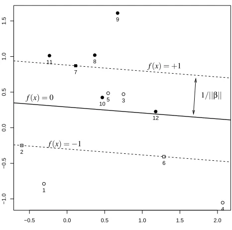
Figure 1: A simple example shows the elements of a SVM model. The “+1” points are solid, the “-1” hollow. C=2, and the width of the soft margin is 2/||β||=2×0.587. Two hollow points{3,5}are misclassified, while the two solid points{10,12}are correctly classified, but on the wrong side of their margin f(x) = +1; each of these hasξi>0. The

three square shaped points{2,6,7}are exactly on the margin.

and its associated classifier

Class(x) =sign[f(x)]. (2)

There are many ways to fit such a linear classifier, including linear regression, Fisher’s linear discriminant analysis, and logistic regression (Hastie et al., 2001, Chapter 4). If the training data are linearly separable, an appealing approach is to ask for the decision boundary {x : f(x) =0}

that maximizes the margin between the two classes (Vapnik, 1996). Solving such a problem is an exercise in convex optimization; the popular setup is

min β0,β

1 2||β||

2_{subject to, for each i: y}

i(β0+xTi β)≥1. (3)

A bit of linear algebra shows that _||1_β_||(β0+xT_i β) is the signed distance from xi to the decision

boundary. When the data are not separable, this criterion is modified to

min β0,β

1 2||β||

2₊_C

∑

n

i=1

ξi, (4)

(3)

-3 -2 -1 0 1 2 3

0.0

0.5

1.0

1.5

2.0

2.5

3.0

Binomial Log-likelihood Support Vector

y f(x)

L

o

ss

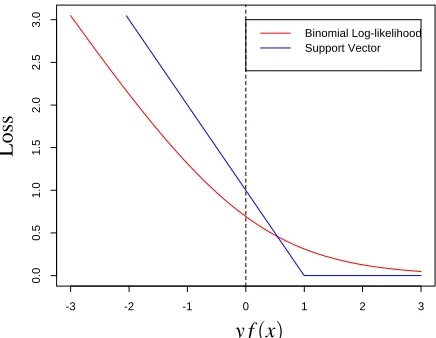
Figure 2: The hinge loss penalizes observation margins y f(x)less than+1 linearly, and is indiffer-ent to margins greater than+1. The negative binomial log-likelihood (deviance) has the same asymptotes, but operates in a smoother fashion near the elbow at y f(x) =1.

Here theξiare non-negative slack variables that allow points to be on the wrong side of their “soft

margin” ( f(x) =±1), as well as the decision boundary, and C is a cost parameter that controls the amount of overlap. Figure 1 shows a simple example. If the data are separable, then for sufficiently large C the solutions to (3) and (4) coincide. If the data are not separable, as C gets large the solution approaches the minimum overlap solution with largest margin, which is attained for some finite value of C.

Alternatively, we can formulate the problem using a Loss +Penalty criterion (Wahba et al.,

2000; Hastie et al., 2001):

min β0,β

n

∑

i=1

[1−yi(β0+βTxi)]++λ 2||β||

2_. ₍₅₎

The regularization parameter λ in (5) corresponds to 1/C, with C in (4). Here the hinge loss L(y,f(x)) = [1−y f(x)]+ can be compared to the negative binomial log-likelihood L(y,f(x)) = log[1+exp(−y f(x))]for estimating the linear function f(x) =β0+βT_{x; see Figure 2.}

This formulation emphasizes the role of regularization. In many situations we have sufficient variables (e.g. gene expression arrays) to guarantee separation. We may nevertheless avoid the maximum margin separator (λ↓0), which is governed by observations on the boundary, in favor of a more regularized solution involving more observations.

This formulation also admits a class of more flexible, nonlinear generalizations

min

f∈H

n

∑

i=1

L(yi,f(xi)) +λJ(f), (6)

where f(x)is an arbitrary function in some Hilbert space

H

, and J(f)is a functional that measures the “roughness” of f in

H

.

The nonlinear kernel SVMs arise naturally in this context. In this case f(x) =β0+g(x), and

(4)

o o o o o o o o o o o o o o o o o o o o o o o o o o o o o o o o o o o o o o o o o o o o o o o o o o o o o o o o o o o o o o o o o o o o o o o _o o o o o o o o o o o o o o o o o o o o o o o o o o o o o o o o o o o o o o o o o o o o o o o o o o o o o o o

o o o

o o o o o o o o o o o o o o o o o o o o o o o o o o o o o o o o o o o o o o o o o o o o o o oo o o o o o o o o o o o o o o o o o o o o o o o

Training Error: 0.160 Test Error: 0.218 Bayes Error: 0.210

Radial Kernel: C=2,γ=1

o o o o o o o o o o o o o o o o o o o o o o o o o o o o o o o o o o o o o o o o o o o o o o o o o o o o o o o o o o o o o o o o o o o o o o o _o o o o o o o o o o o o o o o o o o o o o o o o o o o o o o o o o o o o o o o o o o o o o o o o o o o o o o o

o o o

o o o o o o o o o o o o o o o o o o o o o o o o o o o o o o o o o o o o o o o o o o o o o o oo o o o o o o o o o o o o o o o o o o o o o o o

Training Error: 0.065 Test Error: 0.307 Bayes Error: 0.210

Radial Kernel: C=10,000,γ=1

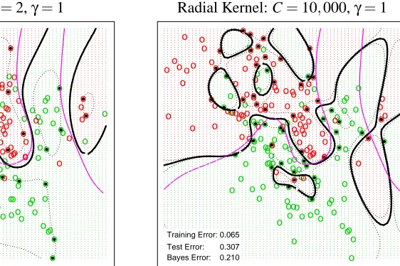
Figure 3: Simulated data illustrate the need for regularization. The 200 data points are generated from a pair of mixture densities. The two SVM models used radial kernels with the scale and cost parameters as indicated at the top of the plots. The thick black curves are the decision boundaries, the dotted curves the margins. The less regularized fit on the right overfits the training data, and suffers dramatically on test error. The broken purple curve is the optimal Bayes decision boundary.

positive-definite kernel K(x,x0). By the well-studied properties of such spaces (Wahba, 1990; Ev-geniou et al., 1999), the solution to (6) is finite dimensional (even if

H

_Kis infinite dimensional), in this case with a representation f(x) =β0+∑n

i=1θiK(x,xi). Consequently (6) reduces to the finite

form

min β0,θ

n

∑

i=1

L[yi,β0+ n

∑

j=1

θiK(xi,xj)] +λ

2

n

∑

j=1

n

∑

j0₌₁

θjθj0K(x_j,x0_j). (7)

With L the hinge loss, this is an alternative route to the kernel SVM; see Hastie et al. (2001) for more details.

It seems that the regularization parameter C (or λ) is often regarded as a genuine “nuisance” in the community of SVM users. Software packages, such as the widely used SVMlight (Joachims, 1999), provide default settings for C, which are then used without much further exploration. A recent introductory document (Hsu et al., 2003) supporting the LIBSVM package does encourage grid search for C.

Figure 3 shows the results of fitting two SVM models to the same simulated data set. The data are generated from a pair of mixture densities, described in detail in Hastie et al. (2001, Chapter 2).1 The radial kernel function K(x,x0) =exp(−γ||x−x0||2₎_{was used, with}γ₌_{1. The model on the left}

is more regularized than that on the right (C=2 vs C=10,000, orλ=0.5 vs λ=0.0001), and

1. The actual training data and test distribution are available from

(5)

1e−01 1e+01 1e+03

0.20

0.25

0.30

0.35

1e−01 1e+01 1e+03 1e−01 1e+01 1e+03 1e−01 1e+01 1e+03

Test Error

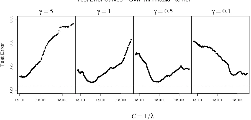
Test Error Curves − SVM with Radial Kernel

γ=5 γ=1 γ=0.5 γ=0.1

C=1/λ

Figure 4: Test error curves for the mixture example, using four different values for the radial kernel parameterγ. Small values of C correspond to heavy regularization, large values of C to light regularization. Depending on the value ofγ, the optimal C can occur at either end of the spectrum or anywhere in between, emphasizing the need for careful selection.

performs much better on test data. For these examples we evaluate the test error by integration over the lattice indicated in the plots.

Figure 4 shows the test error as a function of C for these data, using four different values for the kernel scale parameterγ. Here we see a dramatic range in the correct choice for C (orλ=1/C);

whenγ=5, the most regularized model is called for, and we will see in Section 6 that the SVM is really performing kernel density classification. On the other hand, whenγ=0.1, we would want to choose among the least regularized models.

One of the reasons that investigators avoid extensive exploration of C is the computational cost involved. In this paper we develop an algorithm which fits the entire path of SVM solu-tions[β0(C),β(C)], for all possible values of C, with essentially the computational cost of fitting a single model for a particular value of C. Our algorithm exploits the fact that the Lagrange multi-pliers implicit in (4) are piecewise-linear in C. This also means that the coefficientsβ(C)are also piecewise-linear in C. This is true for all SVM models, both linear and nonlinear kernel-based SVMs. Figure 8 on page 1406 shows these Lagrange paths for the mixture example. This work was inspired by the related “Least Angle Regression” (LAR) algorithm for fitting LASSO models (Efron et al., 2004), where again the coefficient paths are piecewise linear.

These speedups have a big impact on the estimation of the accuracy of the classifier, using a validation dataset (e.g. as in K-fold cross-validation). We can rapidly compute the fit for each test data point for any and all values of C, and hence the generalization error for the entire validation set as a function of C.

(6)

solu-tions (Section 4.3), the nature of the path, in particular at the boundaries, sheds light on the action of the kernel SVM (Section 6).

2. Problem Setup

We use a criterion equivalent to (4), implementing the formulation in (5):

min β,β0

n

∑

i=1 ξi+

λ

2β

T_β ₍₈₎

subject to 1−yif(xi)≤ξi;ξi≥0; f(x) =β0+βTx.

Initially we consider only linear SVMs to get the intuitive flavor of our procedure; we then general-ize to kernel SVMs.

We construct the Lagrange primal function

LP: n

∑

i=1 ξi+

λ

2β

T_β₊

∑

n

i=1

αi(1−yif(xi)−ξi)− n

∑

i=1

γiξi (9)

and set the derivatives to zero. This gives

∂

∂β : β=

1

λ

n

∑

i=1

αiyixi, (10)

∂ ∂β0 :

n

∑

i=1

yiαi=0, (11)

∂ ∂ξi

: αi=1−γi, (12)

along with the KKT conditions

αi(1−yif(xi)−ξi) = 0, (13)

γiξi = 0. (14)

We see that 0≤αi≤1, withαi=1 whenξi>0 (which is when yif(xi)<1). Also when yif(xi)>1,

ξi=0 since no cost is incurred, andαi=0. When yif(xi) =1,αican lie between 0 and 1.2

We wish to find the entire solution path for all values ofλ≥0. The basic idea of our algorithm is as follows. We start withλlarge and decrease it toward zero, keeping track of all the events that occur along the way. Asλdecreases,||β||increases, and hence the width of the margin decreases (see Figure 1). As this width decreases, points move from being inside to outside the margin. Their correspondingαichange fromαi=1 when they are inside the margin (yif(xi)<1) toαi=0 when

they are outside the margin (yif(xi)>1). By continuity, points must linger on the margin (yif(xi) =

1) while theirαi decrease from 1 to 0. We will see that theαi(λ)trajectories are piecewise-linear

inλ, which affords a great computational savings: as long as we can establish the break points, all

(7)

values in between can be found by simple linear interpolation. Note that points can return to the margin, after having passed through it.

It is easy to show that if theαi(λ)are piecewise linear inλ, then bothα0i(C) =Cαi(C)andβ(C)

are piecewise linear in C. It turns out thatβ0(C) is also piecewise linear in C. We will frequently switch between these two representations.

We denote by

I

₊ the set of indices corresponding to yi= +1 points, there being n+=|

I

+|in total. Likewise for

I

₋and n−. Our algorithm keeps track of the following sets (with names inspired

by the hinge loss function in Figure 2):

•

E

={i : yif(xi) =1,0≤αi≤1},

E

for Elbow,

•

L

={i : yif(xi)<1,αi=1},

L

for Left of the elbow,

•

R

={i : yif(xi)>1,αi=0},

R

for Right of the elbow.

3. Initialization

We need to establish the initial state of the sets defined above. Whenλis very large (∞), from (10)

β=0, and the initial values ofβ0and theαidepend on whether n−=n+ or not. If the classes are balanced, one can directly find the initial configuration by finding the most extreme points in each class. We will see that when n−6=n+, this is no longer the case, and in order to satisfy the constraint (11), a quadratic programming algorithm is needed to obtain the initial configuration.

In fact, ourSvmPathalgorithm can be started at any intermediate solution of the SVM optimiza-tion problem (i.e. the soluoptimiza-tion for anyλ), since the values ofαi and f(xi)determine the sets

L,

E

and

R

. We will see in Section 6 that if there is no intercept in the model, the initialization is again trivial, no matter whether the classes are balanced or not. We have prepared some MPEG movies to illustrate the two special cases detailed below. The movies can be downloaded at the web site http://www-stat.stanford.edu/∼hastie/Papers/svm/MOVIE/.

3.1 Initialization: n−=n+

Lemma 1 Forλsufficiently large, all the αi=1. The initial β0∈[−1,1]— any value gives the

same loss∑n_i₌₁ξi=n++n−.

Proof Our proof relies on the criterion and the KKT conditions in Section 2. Sinceβ=0, f(x) =β0. To minimize∑n_i₌₁ξi, we should clearly restrictβ0to[−1,1]. Forβ0∈(−1,1), all theξi>0,γi=0

in (12), and henceαi=1. Picking one of the endpoints, sayβ0=−1, causesαi=1, i∈

I

+, and hence alsoαi=1,i∈

I

−, for (11) to hold.

We also have that for these early and large values ofλ

β= 1

λβ∗whereβ∗=

n

∑

i=1

yixi. (15)

Now in order that (11) remain satisfied, we need that one or more positive and negative examples hit the elbow simultaneously. Hence asλdecreases, we require that∀i yif(xi)≤1 or

yi "

β∗T

xi

λ +β0

#

(8)

0.00 0.05 0.10 0.15 0.20

−1.0

−0.5

0.0

0.5

0.00 0.05 0.10 0.15 0.20

−1.0

−0.5

0.0

0.5

111111111111111111111_{111111111111111111111} 1111111111111111111_11111111

11111111111111111111_{111111111111111111111111111111111111}

111111111111111111111111111111111111_{111111111111111111111111111111111111111} 22222222_22222222

22222222_22222222 22222222_22222222

22222222_222222222

222222222222222222222222222222222222222222222222222222222222222222222222222222222222222222222222222222222222222222222222222222222222222 3333333333

3333333333 333333333333333

333333333333333 33333333333333333

33333333333333 3333333333333333333333333333333333333333

3333333333333333333333333333333333333333 333333333333333333333333333

333333333333

44444444444444444444444444444444444444444444444444444444444444444444444444444444444444444444444444444444444444444444444444444444444444444444444444444444444444444444444444444444444444444444444444444444 5555555555_5555555555

5555555555_5555555555

5555555555_{555555555555555555555555555555555555555555555555555555555555555555555}555555555555555555555555555555555555555555555555555555555555555555555555555555555 6666666666_6666666666

6666666666_6666666666 6666666666_6666666666

6666666666666 666666666666666666_{6666666666666666666666666}

6666666666666666666666666_{66666666666666666666666} 66666666666666_{66666666666666}

66666666 777777777_777777777

777777777_777777777 777777777

777777777_{777777777777777}

7777777777777777777777777_{777777777777777777777777} 777777777777777777777777

77777777777777777777777777777_{77777777777777777777777777777} 8888888888888888888888888888888888888888

8888888888888888888888888888888888888888888888888888888888888888_{8888888888888888888888888}

8888888888888888888888888_{8888888888888888888888888888888888888888888888} 99999999999999999999999999999999999999999999999999999999999999999999999999999999999999999999999999999999999999999999999999999999999999999999999999999999999999999999999999999999999999999999999999999999 0000000000000000000000000000000000000000000000000000000000000000000000000000000000000000000000000000000000000000000000000000000000000000000000000000000000000000000_{0000000000000000000000000000000000000} β0

(

C

)

β

(

C

)

C=1/λ

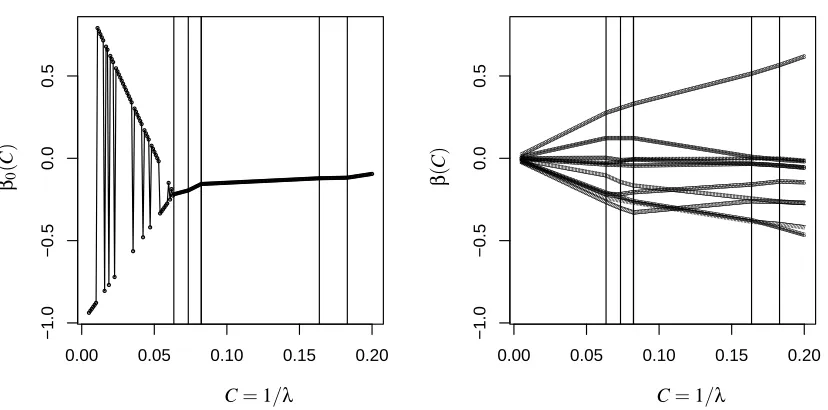
Figure 5: The initial paths of the coefficients in a small simulated dataset with n−=n+. We see the zone of allowable values forβ0shrinking toward a fixed point (20). The vertical lines indicate the breakpoints in the piecewise linear coefficient paths.

or

β0 ≤ 1−β

∗T

xi

λ for all i∈

I

+ (17)

β0 ≥ −1−β

∗T

xi

λ for all i∈

I

−. (18)

Pick i+ =arg maxi∈I+β∗

T

xi and i− =arg mini∈I−β∗

T

xi (for simplicity we assume that these are

unique). Then at this point of entry and beyond for a while we haveαi+ =αi−, and f(xi+) =1 and f(xi−) =−1. This gives us two equations to solve for the initial point of entryλ0andβ0, with solutions

λ0 = β ∗T

xi+−β∗

T

xi−

2 , (19)

β0 = − β

∗T_x

i++β∗

T_x

i−

β∗T_x

i+−β∗

T_x

i−

!

. (20)

(9)

0.00 0.05 0.10 0.15 0.20

0.5

0.6

0.7

0.8

0.9

C

0.00 0.05 0.10 0.15 0.20

−0.4

−0.2

0.0

0.2

C ***_***

***_*** ***_***

***_*** *********_{****************************}

********_{***************} ****************_{****************}

****************_{********************} *****************************

*****************************_{********************************}************

***************************************************************** ********************************* ********

******** ********

**************** ********************************_************

*****************_{*****************} *****************_{*****************}

******_****** ******_******

******************************************************************************************************************************** *********

****** *********

****** ******

****** *********

****** ******

*****************************************************************************************************************************************

**_** **_**

** **_**

**_** **_**

**_** *******_***********

********_******* ***_****

****_**** ******_{***************}

***********************_{***********************} *********** ***************

********** **********

*************** **********

**********

**********************************************************************************************************************************

*****************************************************************************_******** ********_************

************************************************************************************** ********* ****************************************************************************************

*****************************

***********************************************************************************

**********_********** **********_**********

**********_**********

**************************************************************************************************************_{******************************}

0.00 0.05 0.10 0.15 0.20

0.0

0.2

0.4

0.6

0.8

1.0

C

1 1

1

1 1 1

1

1 1

0.00 0.05 0.10 0.15 0.20

−1.0

−0.5

0.0

0.5

1.0

1.5

C

1

2 3

4 5 6 7

8 9 10 11 12

β0

(

C

)

β

(

C

)

α

(

C

)

M

ar

g

in

s

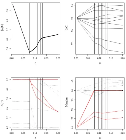
Figure 6: The initial paths of the coefficients in a case where n− <n+. All the n− points are

misclassified, and start off with a margin of−1. Theα∗_i remain constant until one of the points in

I

− reaches the margin. The vertical lines indicate the breakpoints in the

piecewise linearβ(C)paths. Note that theαi(C)are not piecewise linear in C, but rather

(10)

predefined grid of values for λ. The arbitrariness of the initial values is indicated by the zig-zag nature of this path. The breakpoints were found using our exact-path algorithm.

3.2 Initialization: n+>n−

In this case, whenβ=0, the optimal choice forβ0 is 1, and the loss is∑_in₌₁ξi=n−. However, we

also require that (11) holds.

Lemma 2 Withβ∗(α) =∑n

i=1yiαixi, let

{α∗

i} = arg min_α ||β∗(α)||2 (21)

s.t. αi∈[0,1]for i∈

I

+,αi=1 for i∈

I

−, and∑i∈I+αi=n− (22)

Then for someλ0we have that for allλ>λ0,αi=α∗i, andβ=β∗/λ, withβ∗=∑ni=1yiα∗ixi.

Proof The Lagrange dual corresponding to (9) is obtained by substituting (10)–(12) into (9) (Hastie

et al., 2001, Equation 12.13):

LD= n

∑

i=1 αi−

1 2λ

n

∑

i=1

n

∑

i0₌₁

αiαi0y_iy_i0x_ix_i0. (23)

Since we start with β=0, β0 =1, all the

I

₋ points are misclassified, and hence we will have

αi=1∀i∈

I

−, and hence from (11)∑in=1αi=2n−. This latter sum will remain 2n−for a while as

βgrows away from zero. This means that during this phase, the first term in the Lagrange dual is constant; the second term is equal to−₂1_λ||β∗(α)||2_{, and since we maximize the dual, this proves}

the result.

We now establish the “starting point”λ0andβ0when theαistart to change. Letβ∗be the fixed

coefficient direction corresponding toα∗_i (as in (15)):

β∗₌

∑

n

i=1 α∗

iyixi. (24)

There are two possible scenarios:

1. There exist two or more elements in

I

₊with 0<α∗_i <1, or 2. α∗_i ∈ {0,1} ∀i∈

I

₊.

Consider the first scenario (depicted in Figure 6), and supposeα∗_i₊ ∈(0,1) (on the margin). Let

i−=arg mini∈I−β

∗T_x

i. Then since the point i+remains on the margin until an

I

−point reaches its

margin, we can find

λ0 = β ∗T_x

i+−β

∗T_x i−

2 , (25)

identical in form to to (19), as is the correspondingβ0to (20).

For the second scenario, it is easy to see that we find ourselves in the same situation as in Section 3.1—a point from

I

₋ and one of the points in

I

₊ with α∗_i =1 must reach the margin simultaneously. Hence we get an analogous situation, except with i+=arg maxi∈I1

+β

∗T

xi, where

I

1

(11)

3.3 Kernels

The development so far has been in the original feature space, since it is easier to visualize. It is easy to see that the entire development carries through with “kernels” as well. In this case f(x) =

β0+g(x), and the only change that occurs is that (10) is changed to

g(xi) =

1

λ

n

∑

j=1

αjyjK(xi,xj),i=1, . . . ,n, (26)

orθj(λ) =αjyj/λusing the notation in (7).

Our initial conditions are defined in terms of expressions β∗Txi+, for example, and again it is easy to see that the relevant quantities are

g∗(xi+) =

n

∑

j=1 α∗

jyjK(xi+,xj), (27)

where theα∗_i are all 1 in Section 3.1, and defined by Lemma 2 in Section 3.2. Hereafter we will develop our algorithm for this more general kernel case.

4. The Path

The algorithm hinges on the set of points

E

sitting at the elbow of the loss function — i.e on the margin. These points have yif(xi) =1 andαi∈[0,1]. These are distinct from the points

R

to the

right of the elbow, with yif(xi)>1 andαi=0, and those points

L

to the left with yif(xi)<1 and

αi=1. We consider this set at the point that an event has occurred. The event can be either:

1. The initial event, which means 2 or more points start at the elbow, with their initial values of

α∈[0,1].

2. A point from

L

has just entered

E

, with its value ofαiinitially 1.

3. A point from

R

has reentered

E

, with its value ofαiinitially 0.

4. One or more points in

E

has left the set, to join either

R

or

L.

Whichever the case, for continuity reasons this set will stay stable until the next event occurs, since to pass through

E

, a point’sαi must change from 0 to 1 or vice versa. Since all points in

E

have yif(xi) =1, we can establish a path for theirαi.

Event 4 allows for the possibility that

E

becomes empty while

L

is not. If this occurs, then the KKT condition (11) implies that

L

is balanced w.r.t. +1s and -1s, and we resort to the initial condition as in Section 3.1.

We use the subscript `to index the sets above immediately after the `th event has occurred. Suppose |

E

_`|=m, and letα`_i, β`

0 and λ` be the values of these parameters at the point of entry.

Likewise f`is the function at this point. For convenience we defineα0=λβ0, and henceα`₀=λ`β` 0.

Since

f(x) =1

λ

n

∑

j=1

yjαjK(x,xj) +α0 !

(12)

forλ`>λ>λ`+1we can write f(x) =

f(x)−λ` λ f`(x)

+λ`

λ f`(x)

= 1

λ

"

∑

j∈E_`

(αj−α`j)yjK(x,xj) + (α0−α`0) +λ`f`(x)

#

. (29)

The second line follows because all the observations in

L

_`have theirαi=1, and those in

R

` have

theirαi=0, for this range ofλ. Since each of the m points xi∈

E

`are to stay at the elbow, we have

that

1

λ

"

∑

j∈E`

(αj−α`j)yiyjK(xi,xj) +yi(α0−α`0) +λ`

#

=1,∀i∈

E

_`. (30)

Writingδj=α`j−αj, from (30) we have

∑

j∈E`

δjyiyjK(xi,xj) +yiδ0=λ`−λ,∀i∈

E

`. (31)

Furthermore, since at all times∑n_i₌₁yiαi=0, we have that

∑

j∈E`

yjδj=0. (32)

Equations (31) and (32) constitute m+1 linear equations in m+1 unknownsδj, and can be solved.

Denoting by K∗_` the m×m matrix with i jth entry yiyjK(xi,xj)for i and j in

E

`, we have from

(31) that

K∗_`δ+δ0y`= (λ`−λ)1, (33)

where y`is the m vector with entries yi,i∈

E

`. From (32) we have

yT_`δ=0. (34)

We can combine these two into one matrix equation as follows. Let

A`=

0 y`T y` K∗`

, δa=

δ0

δ

,and 1a=

0

1

, (35)

then (34) and (33) can be written

A`δa= (λ`−λ)1a. (36)

If A`has full rank, then we can write

ba=A`−11a, (37)

and hence

αj=α`j−(λ`−λ)bj, j∈ {0} ∪

E

`. (38)

Hence forλ`+1<λ<λ`, theαj for points at the elbow proceed linearly inλ. From (29) we have

f(x) =λ`

λ

h

(13)

where

h`(x) =

∑

j∈E`

yjbjK(x,xj) +b0. (40)

Thus the function itself changes in a piecewise-inverse manner inλ.

If A` does not have full rank, then the solution paths for some of the αi are not unique, and

more care has to be taken in solving the system (36). This occurs, for example, when two training observations are identical (tied in x and y). Other degeneracies can occur, but rarely in practice, such as three different points on the same margin inR2. These issues and some of the related updating and downdating schemes are an area we are currently researching, and will be reported elsewhere.

4.1 Findingλ`+1

The paths (38)–(39) continue until one of the following events occur:

1. One of theαifor i∈

E

`reaches a boundary (0 or 1). For each i the value ofλfor which this

occurs is easily established from (38).

2. One of the points in

L

`or

R

`attains yif(xi) =1. From (39) this occurs for point i at

λ=λ`

f`(xi)−h`(xi)

yi−h`(xi)

. (41)

By examining these conditions, we can establish the largestλ<λ` for which an event occurs, and hence establishλ`+1and update the sets.

One special case not addressed above is when the set

E

becomes empty during the course of the algorithm. In this case, we revert to an initialization setup using the points in

L. It must be the case

that these points have an equal number of +1’s as -1’s, and so we are in the balanced situation as in 3.1.

By examining in detail the linear boundary in examples where p =2, we observed several different types of behavior:

1. If |

E

|=0, than asλdecreases, the orientation of the decision boundary stays fixed, but the margin width narrows asλdecreases.

2. If |

E

|=1 or|

E

|=2, but with the pair of points of opposite classes, then the orientation typically rotates as the margin width gets narrower.

3. If |

E

|=2, with both points having the same class, then the orientation remains fixed, with the one margin stuck on the two points as the decision boundary gets shrunk toward it.

4. If|

E

| ≥3, then the margins and hence f(x)remains fixed, as theαi(λ)change. This implies

that h`= f`in (39).

4.2 Termination

In the separable case, we terminate when

L

becomes empty. At this point, all theξiin (8) are zero,

and further movement increases the norm ofβunnecessarily.

(14)

fixed at a point where∑iξi is as small as possible, and the margin is as wide as possible subject to

this constraint.

4.3 Computational Complexity

At any update event`along the path of our algorithm, the main computational burden is solving the system of equations of size m`=|

E

`|. While this normally involves O(m3_`)computations, since

E

_`₊1 differs from

E

` by typically one observation, inverse updating/downdating can reduce the

computations to O(m2_`). The computation of h`(xi)in (40) requires O(nm`)computations. Beyond

that, several checks of cost O(n)are needed to evaluate the next move.

1e−04 1e−02 1e+00

0 20 40 60 80 100 Size Elbow 1 1 1 1 1 1 1 1 1 1 1 1 1 1 1 1 1 1 1 1 1 1 1 1 1 1 1 1 1 1 1 1 1 1 1 1 1 1 1 1 1 1 1 1 1 1 1 1 1 1 1 1 1 1 1 1 1 1 1 1 1 1 1 1 1 1 1 1 1 1 1 1 1 1 1 1 1 1 1 1 1 1 1 1 1 1 1 1 1 1 1 1 1 1 1 1 1 1 1 1 1 1 1 1 1 1 1 1 1 1 1 1 1 1 1 1 1 1 1 1 1 1 1 1 1 1 1 1 1 1 1 1 1 1 1 1 1 1 1 1 1 1 1 1 1 1 1 1 1 1 1 1 1 1 1 1 1 1 1 1 1 1 1 1 1 1 1 1 1 1 1 1 1 1 1 1 1 1 1 1 1 1 1 1 1 1 1 1 1 1 1 1 1 1 1 1 1 1 1 1 1 1 1 1 1 1 1 1 1 1 1 1 1 1 1 1 1 1 1 1 1 1 1 1 1 1 1 1 1 1 1 1 1 1 1 1 1 1 1 1 1 1 1 1 1 1 1 1 1 1 1 1 1 1 1 1 1 1 1 1 1 1 1 1 1 1 1 1 1 1 1 1 1 1 1 1 1 1 1 1 1 1 1 1 1 1 1 1 1 1 1 1 1 1 1 1 1 1 1 1 1 1 1 1 1 1 1 1 1 1 1 1 1 1 1 1 1 1 1 1 1 1 1 1 1 1 1 1 1 1 1 1 1 1 1 1 1 1 1 1 1 1 1 1 1 1 1 1 1 1 1 1 1 1 1 1 1 1 1 1 1 1 1 1 1 1 1 1 1 1 1 1 1 1 1 1 1 1 1 1 1 1 1 1 1 1 1 1 1 1 1 1 1 1 1 1 1 1 1 1 1 1 1 1 1 1 1 1 1 1 1 1 1 1 1 1 1 1 1 1 1 1 1 1 1 1 1 1 1 1 1 1 1 1 1 1 1 1 1 1 1 1 1 1 1 1 1 1 1 1 1 1 1 1 1 1 1 1 1 1 1 1 1 1 1 1 1 1 1 1 1 1 1 1 1 1 1 1 1 1 1 1 1 2 2 2 2 2 2 2 2 2 2 2 2 2 2 2 2 2 2 2 2 2 2 2 2 2 2 2 2 2 2 2 2 2 2 2 2 2 2 2 2 2 2 2 2 2 2 2 2 2 2 2 2 2 2 2 2 2 2 2 2 2 2 2 2 2 2 2 2 2 2 2 2 2 2 2 2 2 2 2 2 2 2 2 2 2 2 2 2 2 2 2 2 2 2 2 2 2 2 2 2 2 2 2 2 2 2 2 2 2 2 2 2 2 2 2 2 2 2 2 2 2 2 2 2 2 2 2 2 2 2 2 2 2 2 2 2 2 2 2 2 2 2 2 2 2 2 2 2 2 2 2 2 2 2 2 2 2 2 2 2 2 2 2 2 2 2 2 2 2 2 2 2 2 2 2 2 2 2 2 2 2 2 2 2 2 2 2 2 2 2 2 2 2 2 2 2 2 2 2 2 2 2 2 2 2 2 2 2 2 2 2 2 2 2 2 2 2 2 2 2 2 2 2 2 2 2 2 2 2 2 2 2 2 2 2 2 2 2 2 2 2 2 2 2 2 2 2 2 2 2 2 2 2 2 2 2 2 2 2 2 2 2 2 2 2 2 2 2 2 2 2 2 2 2 2 2 2 2 2 2 2 2 2 2 2 2 2 2 2 2 2 2 2 2 2 2 2 2 2 2 2 2 2 2 2 2 2 2 2 2 2 2 2 2 2 2 2 2 2 2 2 2 2 2 2 2 2 2 2 2 2 2 2 2 2 2 2 2 2 2 2 2 2 2 2 2 2 2 2 2 2 2 2 2 2 2 2 2 2 2 2 2 2 2 2 2 2 2 2 2 2 2 2 2 2 2 2 2 2 2 2 2 2 2 2 2 2 2 2 2 2 2 2 2 2 2 2 2 2 2 2 2 2 2 2 2 2 2 2 2 2 2 2 2 2 2 2 2 2 2 2 2 2 2 2 2 2 2 2 2 2 2 2 2 2 2 2 2 2 2 2 2 2 2 2 2 2 2 2 2 2 2 2 2 2 2 2 2 2 2 2 2 2 2 2 2 2 2 2 2 2 2 2 2 2 2 2 2 2 2 2 2 2 2 2 2 2 2 2 2 2 2 2 2 2 2 2 2 2 2 2 2 2 2 2 2 2 2 2 2 2 2 2 2 2 2 2 2 2 2 2 2 2 2 2 2 2 2 2 2 2 2 2 2 2 2 2 2 2 2 2 2 2 2 2 2 2 2 2 2 2 2 2 2 2 2 2 2 2 2 2 2 2 2 2 2 2 2 2 2 2 2 2 2 2 2 2 2 2 2 2 2 2 2 2 2 2 2 2 2 2 2 2 2 2 2 2 2 2 2 2 2 2 2 2 2 2 2 2 2 2 2 2 2 2 2 2 2 2 3 3 3 3 3 3 3 3 3 3 3 3 3 3 3 3 3 3 3 3 3 3 3 3 3 3 3 3 3 3 3 3 3 3 3 3 3 3 3 3 3 3 3 3 3 3 3 3 3 3 3 3 3 3 3 3 3 3 3 3 3 3 3 3 3 3 3 3 3 3 3 3 3 3 3 3 3 3 3 3 3 3 3 3 3 3 3 3 3 3 3 3 3 3 3 3 3 3 3 3 3 3 3 3 3 3 3 3 3 3 3 3 3 3 3 3 3 3 3 3 3 3 3 3 3 3 3 3 3 3 3 3 3 3 3 3 3 3 3 3 3 3 3 3 3 3 3 3 3 3 3 3 3 3 3 3 3 3 3 3 3 3 3 3 3 3 3 3 3 3 3 3 3 3 3 3 3 3 3 3 3 3 3 3 3 3 3 3 3 3 3 3 3 3 3 3 3 3 3 3 3 3 3 3 3 3 3 3 3 3 3 3 3 3 3 3 3 3 3 3 3 3 3 3 3 3 3 3 3 3 3 3 3 3 3 3 3 3 3 3 3 3 3 3 3 3 3 3 3 3 3 3 3 3 3 3 3 3 3 3 3 3 3 3 3 3 3 3 3 3 3 3 3 3 3 3 3 3 3 3 3 3 3 3 3 3 3 3 3 3 3 3 3 3 3 3 3 3 3 3 3 3 3 3 3 3 3 3 3 3 3 3 3 3 3 3 3 3 3 3 3 3 3 3 3 3 3 3 3 3 3 3 3 3 3 3 3 3 3 3 3 3 3 3 3 3 3 3 3 3 3 3 3 3 3 3 3 3 3 3 3 3 3 3 3 3 3 3 3 3 3 3 3 3 3 3 3 3 3 3 3 3 3 3 3 3 3 3 3 3 3 3 3 3 3 3 3 3 3 3 3 3 3 3 3 3 3 3 3 3 3 3 3 3 3 3 3 3 3 3 3 3 3 3 3 3 3 3 3 3 3 3 3 3 3 3 3 3 3 3 3 3 3 3 3 3 3 3 3 3 3 3 3 3 3 3 3 3 3 3 3 3 3 3 3 3 3 3 3 3 3 3 3 3 3 3 3 3 3 3 3 3 3 3 3 3 3 3 3 3 3 3 3 3 3 3 3 3 3 3 3 3 3 3 3 3 3 3 3 3 3 3 3 3 3 3 3 3 3 3 3 3 3 3 3 3 3 3 3 3 3 3 3 3 3 3 3 3 3 3 3 3 3 3 3 3 3 3 3 3 3 3 3 3 3 3 4 4 4 4 4 4 4 4 4 4 4 4 4 4 4 4 4 4 4 4 4 4 4 4 4 4 4 4 4 4 4 4 4 4 4 4 4 4 4 4 4 4 4 4 4 4 4 4 4 4 4 4 4 4 4 4 4 4 4 4 4 4 4 4 4 4 4 4 4 4 4 4 4 4 4 4 4 4 4 4 4 4 4 4 4 4 4 4 4 4 4 4 4 4 4 4 4 4 4 4 4 4 4 4 4 4 4 4 4 4 4 4 4 4 4 4 4 4 4 4 4 4 4 4 4 4 4 4 4 4 4 4 4 4 4 4 4 4 4 4 4 4 4 4 4 4 4 4 4 4 4 4 4 4 4 4 4 4 4 4 4 4 4 4 4 4 4 4 4 4 4 4 4 4 4 4 4 4 4 4 4 4 4 4 4 4 4 4 4 4 4 4 4 4 4 4 4 4 4 4 4 4 4 4 4 4 4 4 4 4 4 4 4 4 4 4 4 4 4 4 4 4 4 4 4 4 4 4 4 4 4 4 4 4 4 4 4 4 4 4 4 4 4 4 4 4 4 4 4 4 4 4 4 4 4 4 4 4 4 4 4 4 4 4 4 4 4 4 4 4 4 4 4 4 4 4 4 4 4 4 4 4 4 4 4 4 4 4 4 4 4 4 4 4 4 4 4 4 4 4 4 4 4 4 4 4 4 4 4 4 4 4 4 4 4 4 4 4 4 4 4 4 4 4 4 4 4 4 4 4 4 4 4 4 4 4 4 4 4 4 4 4 4 4 4 4 4 4 4 4 4 4 4 4 4 4 4 4 4 4 4 4 4 4 4 4 4 4 4 4 4 4 4 4 4 4 4 4 4 4 4 4 4 4 4 4 4 4 4 4 4 4 4 4 4 4 4

γ=0.1

γ=0.5

γ=1

γ=5

λ

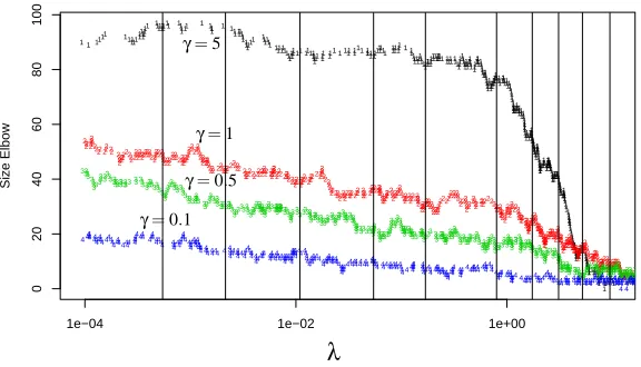
Figure 7: The elbow sizes|

E

_`|as a function ofλ, for different values of the radial-kernel parameter

γ. The vertical lines show the positions used to compare the times withlibsvm.

We have explored using partitioned inverses for updating/downdating the solutions to the elbow equations (for the nonsingular case), and our experiences are mixed. In our R implementations, the computational savings appear negligible for the problems we have tackled, and after repeated updating, rounding errors can cause drift. At the time of this publication, we in fact do not use updating at all, and simply solve the system each time. We are currently exploring numerically stable ways for managing these updates.

Although we have no hard results, our experience so far suggests that the total number Λof moves is O(k min(n+,n−)), for k around 4−6; hence typically some small multiple c of n. If the

average size of

E

_` is m, this suggests the total computational burden is O(cn2m+nm2), which is similar to that of a single SVM fit.

Our R functionSvmPathcomputes all 632 steps in the mixture example (n+=n−=100, radial

(15)

We often wish to make predictions at new inputs. We can also do this efficiently for all values ofλ, because from (28) we see that (modulo 1/λ), these also change in a piecewise-linear fashion inλ. Hence we can compute the entire fit path for a single input x in O(n) calculations, plus an additional O(nq)operations to compute the kernel evaluations (assuming it costs O(q) operations to compute K(x,xi)).

5. Examples

In this section we look at three examples, two synthetic and one real. We examine our running mix-ture example in some more detail, and expose the namix-ture of quadratic regularization in the kernel feature space. We then simulate and examine a scaled-down version of the pn problem—many

more inputs than samples. Despite the fact that perfect separation is possible with large margins, a heavily regularized model is optimal in this case. Finally we fit SVM path models to some microar-ray cancer data.

5.1 Mixture Simulation

In Figure 4 we show the test-error curves for a large number of values ofλ, and four different values forγfor the radial kernel. Theseλ` are in fact the entire collection of change points as described in Section 4. For example, for the second panel, withγ=1, there are 623 change points. Figure 8 [upper plot] shows the paths of all theαi(λ), as well as [lower plot] a few individual examples. An

MPEG movie of the sequence of models can be downloaded from the first author’s website.

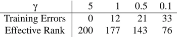
We were at first surprised to discover that not all these sequences achieved zero training errors on the 200 training data points, at their least regularized fit. In fact the minimal training errors, and the corresponding values forγare summarized in Table 1. It is sometimes argued that the implicit

γ 5 1 0.5 0.1

Training Errors 0 12 21 33 Effective Rank 200 177 143 76

Table 1: The number of minimal training errors for different values of the radial kernel scale pa-rameter γ, for the mixture simulation example. Also shown is the effective rank of the 200×200 Gram matrix Kγ.

feature space is “infinite dimensional” for this kernel, which suggests that perfect separation is always possible. The last row of the table shows the effective rank of the kernel Gram matrix K (which we defined to be the number of singular values greater than 10−12). This 200×200 matrix has elements Ki,j=K(xi,xj),i,j=1, . . . ,n. In general a full rank K is required to achieve perfect

separation. Similar observations have appeared in the literature (Bach and Jordan, 2002; Williams and Seeger, 2000).

(16)

1e−04 1e−02 1e+00

0

1

αi

(

λ

)

λ

0 5 10 15

0

1

αi

(

λ

)

λ

Figure 8: [Upper plot] The entire collection of piece-wise linear pathsαi(λ), i=1, . . . ,N, for the

(17)

Writing (7) in matrix form,

min β0,θ

L[y,Kθ] +λ

2θ

T_Kθ, ₍₄₂₎

we reparametrize using the eigen-decomposition of K=UDUT. Let Kθ=Uθ∗whereθ∗=DUTθ. Then (42) becomes

min β0,θ∗

L[y,Uθ∗] +λ

2θ

∗T

D−1θ∗. (43)

Now the columns of U are unit-norm basis functions (in R2) spanning the column space of K;

11111111_{1111111111111111}

111111111111111_{11111111111111111111111111}

11111111111111_{1111111111111111} 1111111111111_{11111111111111}

11111111111_11111111 1111111111₁₁₁₁₁₁

1111111₁₁₁₁₁₁ 11111111

11111111 11111

111 111

1 11

0 50 100 150 200

1e−15

1e−11

1e−07

1e−03

1e+01

Eigenvalue Sequence

Eigenvalue

2

22₂₂

22222 222222

222222₂₂₂₂₂₂

22222₂₂₂₂

222222₂₂₂₂₂

22222₂₂₂₂

22222222 2222222

22222222

222222222

222222

222₂₂₂₂₂

2 22222

22222 2222

2222 222

22222

222222

2222

222₂₂

222 222

22₂₂

22222

22 2₂

222

222222222

2 3

33 33₃₃₃

33

3333₃₃₃

33333₃₃₃

333333

3333

3333333

3333₃₃₃₃

333₃₃

333333

333₃₃₃

3333₃₃₃₃₃₃

333

3333₃₃₃₃₃

33

3333₃₃₃₃

33

333333

33333₃₃₃ 333

333₃₃₃

33

33₃₃₃

33 33

33₃₃₃

3333

333

33333

3333

3333333333333333333333333333333333333333333

3

4 4 4 4 4 44

4 4₄₄

4₄ 444₄

44 4444

4 44

444 44

4₄₄₄ 4 44

44₄₄ 4 4444

4₄ 44

44 4 44

4444 44

4₄ 44

44₄₄₄ 44

444 4 4444

444₄

44444444444444444444444444444444444444444444444444444444444444444444444444444444444444444444444444444444444444444 4 4 γ=0.1

γ=0.5

γ=1

γ=5

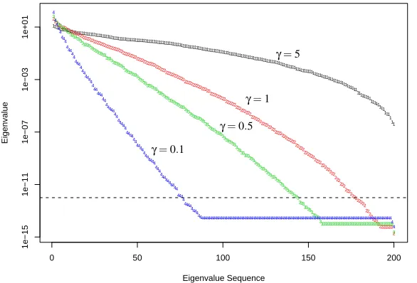
Figure 9: The eigenvalues (on the log scale) for the kernel matrices K_γcorresponding to the four values ofγas in Figure 4. The larger eigenvalues correspond in this case to smoother eigenfunctions, the small ones to rougher. The rougher eigenfunctions get penalized ex-ponentially more than the smoother ones. For smaller values ofγ, the effective dimension of the space is truncated.

from (43) we see that those members corresponding to near-zero eigenvalues (the elements of the diagonal matrix D) get heavily penalized and hence ignored. Figure 9 shows the elements of D for the four values ofγ. See Hastie et al. (2001, Chapter 5) for more details.

5.2 pn Simulation

(18)

We mimic a simulation found in Marron (2003). We have p=50 and n=40, with a 20-20 split of “+” and “-” class members. The xi j are all iid realizations from a N(0,1)distribution, except for

the first coordinate, which has mean +2 and -2 in the respective classes.3 The Bayes classifier in this case uses only the first coordinate of x, with a threshold at 0. The Bayes risk is 0.012. Figure 10 summarizes the experiment. We see that the most regularized models do the best here, not the maximal margin classifier.

Although the most regularized linear SVM is the best in this example, we notice a disturbing aspect of its endpoint behavior in the top-right plot. Althoughβis determined by all the points, the thresholdβ0is determined by the two most extreme points in the two classes (see Section 3.1). This can lead to irregular behavior, and indeed in some realizations from this model this was the case. For values ofλlarger than the initial valueλ1, we saw in Section 3 that the endpoint behavior depends on whether the classes are balanced or not. In either case, asλincreases, the error converges to the estimated null error rate nmin/n.

This same objection is often made at the other extreme of the optimal margin; however, it typi-cally involves more support points (19 points on the margin here), and tends to be more stable (but still no good in this case). For solutions in the interior of the regularization path, these objections no longer hold. Here the regularization forces more points to overlap the margin (support points), and hence determine its orientation.

Included in the figures are regularized linear discriminant analysis and logistic regression mod-els (using the sameλ`sequence as the SVM). Both show similar behavior to the regularized SVM, having the most regularized solutions perform the best. Logistic regression can be seen to assign weights pi(1−pi)to observations in the fitting of its coefficientsβandβ0, where

pi=

1

1+e−β0−βTxi (44)

is the estimated probability of+1 occurring at xi (Hastie and Tibshirani, 1990, e.g.).

• Since the decision boundary corresponds to p(x) =0.5, these weights can be seen to die down in a quadratic fashion from 1/4, as we move away from the boundary.

• The rate at which the weights die down with distance from the boundary depends on||β||; the smaller this norm, the slower the rate.

It can be shown, for separated classes, that the limiting solution (λ↓0) for the regularized logistic regression model is identical to the SVM solution: the maximal margin separator (Rosset et al., 2003).

Not surprisingly, given the similarities in their loss functions (Figure 2), both regularized SVMs and logistic regression involve more or less observations in determining their solutions, depending on the amount of regularization. This “involvement” is achieved in a smoother fashion by logistic regression.

5.3 Microarray Classification

We illustrate our algorithm on a large cancer expression data set (Ramaswamy et al., 2001). There are 144 training tumor samples and 54 test tumor samples, spanning 14 common tumor classes that

(19)

−4 −2 0 2 4 −3 −2 −1 0 1 2 Optimal Margin Optimal Direction SVM Direction + + + + + + + + + + + + + + + + + + + + o o o o o o o o o o_o o o oo o o o o o

−4 −2 0 2 4

−3 −2 −1 0 1 2 Extreme Margin Optimal Direction SVM Direction + + + + + + + + + + + + + + + + + + ++ o o o o o o o o o o o o o o o o o o o o S S S S S S S S S S S S S S S S S S S S S S S S S S S S S S S S S S S S S S S S S S S S S S S S S S S S S S S S S S S S

100 200 300

25 30 35 40 Angle (degrees) R R R R R R R R R R R R R R R R R R R R R R R R R R R R R R R R R R R R R R R R R R R R R R R R R R R R R R R R R R R L L L L L L L L L L L L L L L L L L L L L L L L L L L L L L L L L L L L L L L L L L L L L L L L L L L L L L L L L L L L S S S S S S S S S S S S S S S S S S S S S S S S S S S S S S S S S S S S S S S S S S S S S S S S S S S S S S S S S S S S

100 200 300

0.02 0.03 0.04 0.05 Test Error R R R R R R R R R R R R R R R R R R R R R R R R R R R R R R R R R R R R R R R R R R R R R R R R R R R R R R R R R R R R L L L L L L L L L L L L L L L L L L L L L L L L L L L L L L L L L L L L L L L L L L L L L L L L L L L L L L L L L L L L

λ=1/C λ=1/C

Figure 10: pn simulation. [Top Left] The training data projected onto the space spanned by the

(20)

account for 80% of new cancer diagnoses in the U.S.A. There are 16,063 genes for each sample. Hence p=16,063 and n=144. We denote the number of classes by K=14. A goal is to build a classifier for predicting the cancer class of a new sample, given its expression values.

We used a common approach for extending the SVM from two-class to multi-class classifica-tion:

1. Fit K different SVM models, each one classifying a single cancer class (+1) versus the rest (-1).

2. Let[f₁λ(x), . . . ,f_Kλ(x)]be the vector of evaluations of the fitted functions (with parameterλ) at a test observation x.

3. Classify Cλ(x) =arg maxk f_kλ(x).

Other, more direct, multi-class generalizations exist (Rosset et al., 2003; Weston and Watkins, 1998); although exact path algorithms are possible here too, we were able to implement our ap-proach most easily with the “one vs all” strategy above. Figure 11 shows the results of fitting this family of SVM models. Shown are the training error, test error, as well as 8-fold balanced cross-validation.4 The training error is zero everywhere, but both the test and CV error increase sharply when the model is too regularized. The right plot shows similar results using quadratically regularized multinomial regression (Zhu and Hastie, 2004).

Although the least regularized SVM and multinomial models do the best, this is still not very good. With fourteen classes, this is a tough classification problem.

It is worth noting that:

• The 14 different classification problems are very “lop-sided”; in many cases 8 observations in one class vs the 136 others. This tends to produce solutions with all members of the small class on the boundary, a somewhat unnatural situation.

• For both the SVM and the quadratically regularized multinomial regression, one can reduce the logistics by pre-transforming the data. If X is the n×p data matrix, with pn, let its

singular-value decomposition be UDVT. We can replace X by the n×n matrix XV=UD=R

and obtain identical results (Hastie and Tibshirani, 2003). The same transformation V is applied to the test data. This transformation is applied once upfront, and the transformed data is used in all subsequent analyses (i.e. K-fold cross-validation as well).

6. No Intercept and Kernel Density Classification

Here we consider a simplification of the models (6) and (7) where we leave out the intercept term

β0. It is easy to show that the solution for g(x)has the identical form as in (26):

g(x) = 1

λ

n

∑

j=1

αjyjK(x,xj). (45)

However, f(x) =g(x)(or f(x) =βT_{x in the linear case), and we lose the constraint (11) due to the}

intercept term.

This also adds considerable simplification to our algorithm, in particular the initial conditions.

(21)

1 10 100 1000 10000

0.0

0.1

0.2

0.3

0.4

0.5

Misclassification Rates

SVM

Train Test 10−fold CV

1e−02 1e+00 1e+02 1e+04

0.0

0.1

0.2

0.3

0.4

0.5

Misclassification Rates

Multinomial Regression

λ λ

Figure 11: Misclassification rates for cancer classification by gene expression measurements. The left panel shows the the training (lower green), cross-validation (middle black, with standard errors) and test error (upper blue) curves for the entire SVM path. Although the CV and test error curves appear to have quite different levels, the region of interesting behavior is the same (with a curious dip at about λ=3000). Seeing the entire path leaves no guesswork as to where the region of interest might be. The right panel shows the same for the regularized multiple logistic regression model. Here we do not have an exact path algorithm, so a grid of 15 values ofλis used (on a log scale).

• It is easy to see that initiallyαi =1∀i, since f(x) is close to zero for largeλ, and hence all

points are in

L. This is true whether or not n

₋=n+, unlike the situation when an intercept is present (Section 3.2).

• With f∗(x) =∑n

j=1yjK(x,xj), the first element of

E

is i∗ =arg maxi|f∗(xi)|, with λ1 =

|f∗(xi∗)|. Forλ∈[λ1,∞), f(x) = f∗(x)/λ.

• The linear equations that govern the points in

E

are similar to (33):

K∗_`δ= (λ`−λ)1, (46)

(22)

else to class -1. But

f∗(x) =

∑

j∈I+

K(x,xj)−

∑

j∈I−

K(x,xj)

= n· n+ n ·

1

n+ _j

∑

_∈I+

K(x,xj)−

n−

n ·

1

n− _j

∑

_∈I−

K(x,xj) !

(47)

∝ π+h+(x)−π−h−(x). (48)

In other words, this is the estimated Bayes decision rule, with h+the kernel density (Parzen window) estimate for the + class,π+the sample prior, and likewise for h−(x)andπ−. A similar observation

is made in Sch¨olkopf and Smola (2001), for the model with intercept. So at this end of the regular-ization scale, the kernel parameterγplays a crucial role, as it does in kernel density classification. Asγincreases, the behavior of the classifier approaches that of the 1-nearest neighbor classifier. For very smallγ, or in fact a linear kernel, this amounts to closest centroid classification.

Asλis relaxed, theαi(λ)will change, giving ultimately zero weight to points well within their

own class, and sharing the weights among points near the decision boundary. In the context of nearest neighbor classification, this has the flavor of “editing”, a way of thinning out the training set retaining only those prototypes essential for classification (Ripley, 1996).

All these interpretations get blurred when the interceptβ0is present in the model.

For the radial kernel, a constant term is included in span{K(x,xi)}n1, so it is not strictly necessary

to include one in the model. However, it will get regularized (shrunk toward zero) along with all the other coefficients, which is usually why these intercept terms are separated out and freed from regularization. Adding a constant b2to K(·,·)will reduce the amount of shrinking on the intercept (since the amount of shrinking of an eigenfunction of K is inversely proportional to its eigenvalue; see Section 5). For the linear SVM, we can augment the xivectors with a constant element b, and

then fit the no-intercept model. The larger b, the closer the solution will be to that of the linear SVM with intercept.

7. Discussion

Our work on the SVM path algorithm was inspired by earlier work on exact path algorithms in other settings. “Least Angle Regression” (Efron et al., 2002) shows that the coefficient path for the sequence of “lasso” coefficients (Tibshirani, 1996) is piecewise linear. The lasso solves the following regularized linear regression problem,

min β0,β

n

∑

i=1

(yi−β0−xTi β)2+λ|β|, (49)

where|β|=∑p_j₌₁|βj|is the L1norm of the coefficient vector. This L1 constraint delivers a sparse

solution vectorβ_λ; the largerλ, the more elements ofβ_λare zero, the remainder shrunk toward zero. In fact, any model with an L1 constraint and a quadratic, piecewise quadratic, piecewise linear, or

mixed quadratic and linear loss function, will have piecewise linear coefficient paths, which can be calculated exactly and efficiently for all values ofλ(Rosset and Zhu, 2003). These models include, among others,

(23)

• The L1constrained support vector machine (Zhu et al., 2003).

The SVM model has a quadratic constraint and a piecewise linear (“hinge”) loss function. This leads to a piecewise linear path in the dual space, hence the Lagrange coefficientsαi are piecewise

linear.

Other models that would share this property include

• Theε-insensitive SVM regression model

• Quadratically regularized L1regression, including flexible models based on kernels or

smooth-ing splines.

Of course, quadratic criterion + quadratic constraints also lead to exact path solutions, as in the classic case of ridge regression, since a closed form solution is obtained via the SVD. However, these paths are nonlinear in the regularization parameter.

For general non-quadratic loss functions and L1 constraints, the solution paths are typically

piecewise non-linear. Logistic regression is a leading example. In this case, approximate path-following algorithms are possible (Rosset, 2005).

The general techniques employed in this paper are known as parametric programming via active sets in the convex optimization literature (Allgower and Georg, 1992). The closest we have seen to our work in the literature employ similar techniques in incremental learning for SVMs (Fine and Scheinberg, 2002; Cauwenberghs and Poggio, 2001; DeCoste and Wagstaff, 2000). These authors do not, however, construct exact paths as we do, but rather focus on updating and downdating the solutions as more (or less) data arises. Diehl and Cauwenberghs (2003) allow for updating the parameters as well, but again do not construct entire solution paths. The work of Pontil and Verri (1998) recently came to our notice, who also observed that the lagrange multipliers for the margin vectors change in a piece-wise linear fashion, while the others remain constant.

TheSvmPathhas been implemented in theRcomputing environment (contributed librarysvmpath at CRAN), and is available from the first author’s website.

Acknowledgments

The authors thank Jerome Friedman for helpful discussions, and Mee-Young Park for assisting with some of the computations. They also thank two referees and the associate editor for helpful comments. Trevor Hastie was partially supported by grant DMS-0204162 from the National Science Foundation, and grant RO1-EB0011988-08 from the National Institutes of Health. Tibshirani was partially supported by grant DMS-9971405 from the National Science Foundation and grant RO1-EB0011988-08 from the National Institutes of Health.

References

Eugene Allgower and Kurt Georg. Continuation and path following. Acta Numerica, pages 1–64, 1992.

Francis Bach and Michael Jordan. Kernel independent component analysis. Journal of Machine

(24)

Gert Cauwenberghs and Tomaso Poggio. Incremental and decremental support vector machine learning. In Advances in Neural Information Processing Systems (NIPS 2000), volume 13. MIT Press, Cambridge, MA, 2001.

Dennis DeCoste and Kiri Wagstaff. Alpha seeding for support vector machines. In Proceedings of

the Sixth ACM SIGKDD International Conference on Knowledge Discovery and Data Mining,

pages 345–349. ACM Press, 2000.

Christopher Diehl and Gert Cauwenberghs. SVM incremental learning, adaptation and optimiza-tion. In Proceedings of the 2003 International Joint Conference on Neural Networks, pages 2685–2690, 2003. Special series on Incremental Learning.

Brad Efron, Trevor Hastie, Iain Johnstone, and Robert Tibshirani. Least angle regression. Technical report, Stanford University, 2002.

Brad Efron, Trevor Hastie, Iain Johnstone, and Robert Tibshirani. Least angle regression. Annals

of Statistics, 2004. (to appear, with discussion).

Theodorus Evgeniou, Massimiliano Pontil, and Tomaso Poggio. Regularization networks and sup-port vector machines. Advances in Computational Mathematics, Volume 13, Number 1, pages 1-50, 2000.

Shai Fine and Katya Scheinberg. Incas: An incremental active set method for SVM. Technical report, IBM Research Labs, Haifa, 2002.

Trevor Hastie and Robert Tibshirani. Generalized Additive Models. Chapman and Hall, 1990.

Trevor Hastie, Robert Tibshirani, and Jerome Friedman. The Elements of Statistical Learning; Data

Mining, Inference and Prediction. Springer Verlag, New York, 2001.

Trevor Hastie and Rob Tibshirani. Efficient quadratic regularization for expression arrays. Technical report, Stanford University, 2003.

Chih-Wei Hsu, Chih-Chung Chang, and Chih-Jen Lin. A practical guide to support vector classifica-tion. Technical report, Department of Computer Science and Information Engineering, National Taiwan University, Taipei, 2003. http://www.csie.ntu.edu.tw/∼cjlin/libsvm/.

Thorsten Joachims. Practical Advances in Kernel Methods — Support Vector Learn-ing, chapter Making large scale SVM learning practical. MIT Press, 1999. See http://svmlight.joachims.org.

Steve Marron. An overview of support vector machines and kernel methods. Talk, 2003. Available from author’s website: http://www.stat.unc.edu/postscript/papers/marron/Talks/.

Massimiliano Pontil and Alessandro Verri. Properties of support vector machines. Neural

Compu-tation, 10(4):955–974, 1998.

(25)

B. D. Ripley. Pattern recognition and neural networks. Cambridge University Press, 1996.

Saharon Rosset. Tracking curved regularized optimization solution paths. In Advances in Neural

Information Processing Systems (NIPS 2004), volume 17. MIT Press, Cambridge, MA, 2005. to

appear.

Saharon Rosset and Ji Zhu. Piecewise linear regularized solution paths. Technical report, Stanford University, 2003. http://www-stat.stanford.edu/∼saharon/papers/piecewise.ps. Saharon Rosset, Ji Zhu, and Trevor Hastie. Margin maximizing loss functions. In Advances in

Neural Information Processing Systems (NIPS 2003), volume 16. MIT Press, Cambridge, MA,

2004.

Bernard Sch¨olkopf and Alex Smola. Learning with Kernels: Support Vector Machines,

Regular-ization, OptimRegular-ization, and Beyond (Adaptive Computation and Machine Learning). MIT Press,

2001.

Robert Tibshirani. Regression shrinkage and selection via the lasso. Journal of the Royal Statistical

Society B., 58:267–288, 1996.

Vladimir Vapnik. The Nature of Statistical Learning. Springer-Verlag, 1996.

G. Wahba. Spline Models for Observational Data. SIAM, Philadelphia, 1990.

G. Wahba, Y. Lin, and H. Zhang. Gacv for support vector machines. In A.J. Smola, P.L. Bartlett, B. Sch¨olkopf, and D. Schuurmans, editors, Advances in Large Margin Classifiers, pages 297– 311, Cambridge, MA, 2000. MIT Press.

J. Weston and C. Watkins. Multi-class support vector machines, 1998. URL

citeseer.nj.nec.com/8884.html.

Christopher K. I. Williams and Matthias Seeger. The effect of the input density distribution on kernel-based classifiers. In Proceedings of the Seventeenth International Conference on Machine

Learning, pages 1159–1166. Morgan Kaufmann Publishers Inc., 2000.

Ji Zhu and Trevor Hastie. Classification of gene microarrays by penalized logistic regression.

Bio-statistics, 2004. (to appear).