Unsteady Formulations for Stagnation Point Flow Towards a Stretching and Shrinking Sheet with Prescribed Surface Heat Flux and Viscous Dissipation

http://www.sciencepublishinggroup.com/j/ijfmts doi: 10.11648/j.ijfmts.20170302.11

ISSN: 2469-8105 (Print); ISSN: 2469-8113 (Online)

Unsteady Formulations for Stagnation Point Flow Towards

a Stretching and Shrinking Sheet with Prescribed Surface

Heat Flux and Viscous Dissipation

Okey Oseloka Onyejekwe

Computational Science Program, Addis Ababa University, Arat Kilo Campus, Addis Ababa, Ethiopia

Email address:

okuzaks@yahoo.com

To cite this article:

Okey Oseloka Onyejekwe. Unsteady Formulations for Stagnation Point Flow Towards a Stretching and Shrinking Sheet with Prescribed Surface Heat Flux and Viscous Dissipation. International Journal of Fluid Mechanics & Thermal Sciences. Vol. 3, No. 2, 2017, pp. 16-24. doi: 10.11648/j.ijfmts.20170302.11

Received: December 12, 2016; Accepted: December 27, 2016; Published: April 24, 2017

Abstract: The unsteady stagnation point flow and heat transfer with prescribed flux towards a stretching and shrinking sheet

with viscous dissipation is studied. Similarity transformation is adopted to initially convert the governing differential equations into nonlinear ordinary differential equations. The two-point boundary value ordinary differential equations (ODE) are subsequently converted into partial differential equations by introducing a time-marching scheme. A Crank-Nicolson Newton-Richtmeyer scheme is employed to discretize the resulting equations. Initial guesses are made for the dependent variables and the solution advanced in time until temporal variations of the scalar profile are diminished and the steady-state solutions satisfy the similarity equations. A variation of the heat flux at one of the boundaries produced noticeable variations in the temperature field that can be related to the magnitude of the Prandtl number and velocity ratio parameter.

Keywords: Stagnation Point Flow, Heat Transfer, Prescribed Flux, Crank-Nicolson-Newton-Richtmeyer,

Time Marching Scheme, Steady State, Prandtl Number, Stretching and Shrinking Sheet

1. Introduction

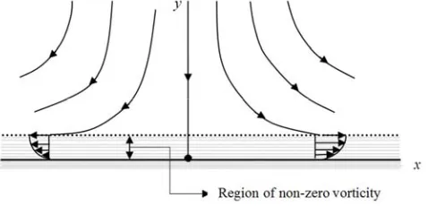
The impact of a viscous fluid on a solid object (Fig. 1) constitutes a prototypical stagnation point flow. Stagnation point flow and heat transfer with prescribed flux have continued to receive considerable attention over the years because of their wide application. The heat transfer over a surface becomes quite interesting when the heat flux boundary condition is taken into account particularly for those problems involving the cooling of electrical and nuclear components, space shuttle re-entry into the earth’s atmosphere, melt-spinning processes etc. This class of problems often encounters rapid heat-flux changes, and possible meltdown hence overheating and burnout constitute very important design considerations. As a result, accurate prediction of the temperature profile becomes vital (Bejan [1]).

The study of viscous flow near a solid object can be traced back to Hiemenz [2] similarity analysis. That is why the stagnation point flow is sometimes referred to as Hiemenz

Crane [6], while the mass transfer effect including suction and blowing was investigated by Gupta and Gupta [7]. Chiam [8] studied the stagnation point flow towards a stretching sheet when the stretching velocity is identical to the free stream velocity. In a similar work, Sakiadis [9, 10] considered the case where the stretched surface was assumed to move with uniform velocity while Mahapatra and Gupta [11] found out that the profile of the boundary layer is a function of the stretching sheet parameters and the angle of incidence. Several other authors can be credited for work in this area. Dulal and Hiremath [12] studied the heat transfer characteristics in a laminar boundary layer flow of an incompressible viscous fluid over an unsteady stretching sheet placed in a porous medium in the presence of viscous dissipation and internal absorption or generation of heat. Relevant references in this area can be found in the books by Ingham and Pop [13], Nield and Bejan [14].

Figure 1. Stagnation point flow.

Relating heat transfer to fluid flow has provided a link between the application of fluid numerical simulation to the industry, This can be observed in such diverse areas as navigation, aviation, rocket propulsion, space exploration, ship building, food processing, and auto manufacture to mention just a few. The heat transfer characterisitcs of a stretching sheet becomes significantly important when the heat flux boundary condition is taken into consideration. Dutta et al. [15] examined the effects of uniform heat flux on the temperature field due to stretching. A similar study was carried out by Alli and Magyari [16] for power-law velocity and temperature distributions. The effect of a magneto-hydrodynamic (MHD) flow on a stretching sheet was studied by Ishak et al. [17]. Similar work was carried out by Anderson [18] his work was later extended with the inclusion of mass transfer by Char [19]. Mahapatra and Nandy [20] provided a momentum and heat transfer solution involving a shrinking sheet for the case of an MHD axisymmetric stagnation point flow. Further work on hydromagnetic flows includes those of Makinde and Charles [21], Makonde [22]. Conjugate convective flows apply in cases involving internal heat generation. These often lead to obtaining useful design parameters [23, 24, and 25].

The aim of this study is to numerically investigate the problem of an unsteady stagnation point flow towards a stretching and shrinking sheet with prescribed surface heat flux and viscous dissipation. The governing differential

equation is obtained from the vorticity transport equation and converted into its third order stream function analog. By using a combination of analytic techniques, non-dimensionalization and appropriate boundary conditions it was possible to arrive at a second order nonlinear transient partial differential equation. The resulting system was solved to steady state by an implicit finite difference Crank-Nicolson-Newton-Richtmeyer scheme. The effects of various non-dimensionless parameters on the flow and heat transfer profiles are presented graphically and discussed.

2. Mathematical Formulations

We seek the governing equation for boundary layer flow towards a stagnation point flow (Fig. 1). The x and y axes are taken along the normal and along a shrinking stretching surface. It is assumed that the free stream velocity is given by

( )

U_∞ x =

ς

x and that the plate is stretched or shrunk with a velocity uw

( )

x =ℓx where ς and ℓ constants are U∞,uw are the freestream and x-component velocity. Under this assumptions we can define the velocity ratio as ζ =υ_ℓ. We start by developing the stream function equation via the vorticity transport. The condition for its existence is that the flow is incompressible. Starting from the steady, two dimensional form of the vorticity equation

2

ω ν ω •∇ = ∇

u and relating the streamfunction to the vorticity u=∂ψ_∂y, v= −∂ψ_∂x , The vorticity vector is expressed as:

ω

= −∇2

ψ

k and when substituted in the vorticity transport equation yields a fourth order equation partial differential equation for the stream function:

4 4 4

4 2 2 4

3 3 3 3

3 2 3 2

2

x x y y

y x x y x y x y

ψ ψ ψ

ν

ψ ψ ψ ψ ψ ψ

_{∂ ∂ ∂} 

+ +

 

_{∂ ∂ ∂ ∂} 

 

   

∂ ∂ ∂ ∂ ∂ ∂

= _ + _− _ + _

∂ ∂ ∂ ∂  ∂ ∂ ∂ ∂ 

(1)

Boundary Conditions:

Two boundary conditions on follow from the no-slip boundary constraint at the surface. The other two concur with the approach of the viscous-flow solution to inviscid flow far enough from the surface.

0 0, 0

at y

y x

ψ ψ

∂ ∂

= = =

∂ ∂ (2a)

,

as y Ax Ay

y x

ψ ψ

∂ ∂

→ ∞ → →

∂ ∂ (2b)

where A=2ψ₀ and ψ₀ is a constant in the inviscid flow solution. Because the first derivative of the streamfunction approaches a constant value ‘A’ asymptotically, we can deduce that its second derivative approaches zero as y

( )

x y

,

ψ

approaches infinity. This observation follows the logic that once a derivative of a function approaches a constant value, all higher order derivatives of that function will approach zero asymptotically. We make a further assumption that the streamfunction comprises both the viscous and inviscid components of flow and as a result; it can be expressed as

( ) ( )

x F y

ψ ϕ

= . Substituting this assumed form of ψ into equation (1) yields explicit equations for the viscous and inviscid regions namely:

ϕ

( )

x = Ax for the inviscid region and for the viscous component, we have the following third-order ordinary differential equation (ODE)

2

3 2

3 2 1 0

d F d F dF

A dy dy dy

ν _ϕ  

+ −  + =

  (3)

With accompanying boundary conditions:

( )

'

( )

0 0 0 0 0

at y= F = F = (4a)

( )

'

1

as y→ ∞ F y → (4b) We adopt Wilcox [26] approach, and introduce the following dimensionless independent and dependent variables

η

=y A

_ν

, f

( )

η

= A

_ν

F y

( )

into equations (3) and (4) to produce:

2

3 2

3 2 1 0

d f d f df

f

dy

dy dy

 

+ −  + =

  (5)

with the following boundary conditions

( )

'

( )

0 0 0 0 0

at y= f = f = (6a)

( )

( )

' _1, '' ₀

as y→ ∞ f y → f y → (6b) Equation (5) is the so called Hiemenz equation. A slightly different approach has been adopted for its derivation. One of the reasons for this is the relative ease with which boundary conditions are handled as well as the avoidance of an iterative procedure to arrive at an appropriate initial condition. Equation (5) facilitates the computation of the velocity field, but for many computations, we also need the pressure field. To initiate this, we make another assumption that the pressure comprises the static and dynamic components and can be described as follows:

( ) ( )

2 0

1 2

p − =p ρA _χ x +F y _ (7) For the classical case of stagnation pressure, at x= =y 0,

( )

₀ 0

y

F y

= = , and the dynamic component is completely

obviated. But we relax the conditions a little bit by considering the fact that as with velocity we expect the pressure to approach the inviscid flow solution in the limit as y→ ∞, given this criterion, the pressure should satisfy the

condition:

2 2 2

0 1 2

p→p − ρA _x +y _ as y→ ∞ (8)

Since a clear concept of the pressure dynamics has been determined, we need an explicit equation for pressure to validate our assumptions. Taking the divergence of the momentum in a two-dimensional form of the Navier-Stokes equation and after rearranging terms, we obtain the Poisson equation for pressure

2 2

2

2

u v u v

p

x y y x

ρ∂  ∂  ∂ ∂  ∇ = −   +  +

∂ ∂ ∂ ∂

    

 

(9)

Though it can be assumed that once the velocity field has been calculated from the streamfunction values, equation(9) can be solved to yield the pressure, nevertheless, it still has to be put in a form that satisfies the physics of the flow as dictated by equations (7) and (8). Equation (7) is further expanded as follows:

( )

2

x x

χ = (10a)

and the function Y y

( )

satisfies: 2 2

2 4 2

d Y dF

dy dy

 

=   −

  (10b)

with the following boundary conditions:

( )

( )

0, 0 0, dY 2

at y Y as y y

dy

= = → ∞ ∞ → (11)

Equation (11) guarantees that p₀ be the true stagnation pressure while the pressure gradient matches that of the inviscid flow in a region far above the surface. In order to complete our solution of the pressure equation, we need to recast equation (10b) into its dimensionless form. We define:

( )

A

( )

P η Y y

η

= and substituting into equation (10b) we obtain:

2 2

2 4 2

d P df

dy dη

 

=   −

  (12)

accompanied by the following boundary conditions

( )

0 0 dP 2

P as

dη η η

= → → ∞ (13)

( )

₂df 2

( )

P f

d

η η

η

= + (14)

We note that the original equation (equation (1)) for the streamfunction was fourth order and represents the viscous analog of the Laplace’s equation for the streamfunction. In addition it satisfies the continuity equation automatically. After integrating once, equation (1) was reduced to third order ODE (equation 5). The overriding approach found in literature is to reduce the governing third order ODE to systems of lower order Odes before applying numerical techniques like the Runge Kutta method. We adopt a different approach here by reducing equation (5) to its second order analog before adopting a time marching procedure. We recall that the dimensionless streamfunction is related to the

( )

'_.

horizontal velocity u η = f This facilitates the formulation of a time marching scheme

2 2

2

1

u u u

f u

t η η

∂ ₋ ∂ _{= − +} ∂

∂ ∂ ∂ (15)

with the boundary conditions:

( )

0 0,

( )

0 0,

( )

1

f = u = u

η

→ =U as

η

→ ∞ (16a) For an initial condition, a guess is made by assuming a quadratic profile for the velocity profile near the surface of the plate

( )

2 0 3 , 3 3 1, u η _η η _η   _{≤ ≤}   =  _{≤ ≤ ∞}   (16b)

Next we consider the boundary layer equation for heat transfer

2 2

2 p

T T T u

c u v k

x y y y

ρ  ∂ + ∂ = ∂ +µ∂ 

∂ ∂ ∂ ∂

    (17a)

where ρ is the density, c_p is the specific heat, µ is the kinematic viscosity, T is the temperature, x, y are the independent variables. The boundary conditions for the velocity and temperature fields are

0 T 0

at y u v

y

∂

= = = _∂ = (17b)

1

,

as y→ ∞ u→U T →T (17c) To solve the energy equation we obtain the velocity field from the solution of the momentum equation. These are then substituted into equation (16) in terms of the similarity variables

and f

η . We initiate this process by converting equation (16) and (17) into dimensionless forms by introducing:

(

)

' '

1

2 0.5

2

, , 0.5

2

T T u

f f f

U U U c x ν θ η ν − = = = −      

to finally obtain a dimensionless energy equation together with the boundary conditions:

( )

2 ₂

'' 2

1

Pr 2 Pr

2 d d f f d d

θ

θ

η

η

+ = − (18)

0 0, 0

at η θ as η θ

η ∂

= = → ∞ →

∂ (19)

3. Discretization

For this study, we have elected to convert equation (18) to a time marching numerical scheme by introducing a temporal derivative.

We employ the Crank-Nicolson Newton-Richtmeyer scheme for discretization, whose general form for a one-dimensional partial differential equation for nonlinear diffusion, convection and source term is given as:

( )

( )

( )

( )

( )

( )

1 2

1 2 3

1

1 2 3

1 2 1 2 k k i k i

t x x x

x x x

φ _{ϑ φ} φ _{ϑ φ} φ _{ϑ φ φ}

φ φ

ϑ φ ϑ φ ϑ φ φ

+ +   ∂ ∂ ∂ ∂     =  + +  +     ∂ ∂ ∂ ∂        _{∂ ∂}  _∂   + +  _{∂ ∂}  _∂       (20) where

( )

k 1

( )

k

( )

k

i i i

t

x x t x

φ φ φ

ϑ φ ∂ + ϑ φ ∂ ∂ ϑ φ ∂

     

= + ∆  

 _∂   _∂  _{∂ ∂}

      (21a)

( )

k 1

( )

k

i i

k k k k

i i i

i

x x

t

t x x t

φ φ

ϑ φ ϑ φ

ϑ φ φ _ϑ φ

φ + ∂ ∂     =  _∂   _∂      _{∂  ∂  ∂   ∂  ∂ }    +∆       +      ∂ ∂  ∂  ∂  ∂        (21b)

Using a forward difference for the time derivative:

( )

1

( )

1 1

k k

i i

k k k

k k i

i i i i x x x x φ φ

ϑ φ ϑ φ

φ

ϑ φ _{φ ϑ}

φ + + + ∂ ∂     =  _∂   _∂        _∂  _∂  _∂∆ +    ∆ + _ _ ∂ ∂  ∂     (21c) Similarly

[ ]

1

[ ]

1 1

k

k k k k k k

i i i i

i i

i

ϑ

ϑφ + ₌ ϑφ _+∂_φ_ φ φ_∆ + _{+ ∆}ϑ φ + ∂

  (21d)

Without any loss in generality; assume

ϑ φ

( )

=

φ

, then equation (20) can be written as:

(

1

)

1

1 k

k k k

i

k k

i i

i i i

x x x x

φ

φ φ φ

φ φ φ φ

+ + + ∂ ∆ ∂ ∂ ∂       = + +  ∆  _∂   _∂  _{∂ ∂}

The diffusion term can now be obtained as follows:

(

)

(

)

1 2 1 1 2 1

2

k k k k k k

k

i i i i i i

i

x x x

φ φ φ φ φ φ

φ

φ + + − − − − −

∂  ∂  =

 

∂  ∂  ∆ (21f)

By the same token

(

)

(

)

1 2 1 1 2 1

2

k k k k k k k

k _{i i i i i i}

k i i

i

x x x

φ φ φ φ φ φ

φ

φ + ∆ + − ∆ − − ∆ − ∆ −

 _∂∆ 

∂_{  =}

 

∂  ∂  ∆

(21g)

(

)(

) (

)(

)

1

1 1 1 1

1 1 1 1

2

k i

k k k k k k k k

i i i i i i i i

x x

x

φ φ

φ φ φ φ φ φ φ φ

+

+ + + +

+ + − −

∂  ∂ 

∆ =

 

∂  ∂ 

∆ + ∆ − − ∆ + ∆ −

∆

(21h)

Following this approach, a nonlinear reaction term is discretized as:

( )

( )

_{( )}

1

1 ₁

k i

k k

i i

k

i _{k k}

i i

t t

t t

χ

χ χ

χ

χ φ

φ φ

φ _φ

χ φ φ

φ

+

− ₊

∂ ϒ

_ϒ  _{= ϒ}  _{+ ∆}

    _∂

 

∂ ϒ _∂

 

= ∆ = ϒ ϒ ∆

∂ ∂

 

 

(21i)

where ϒ is the reaction coefficient, and χ is the power to which the nonlinear term is raised. We note that ∆

φ

_ik+1 is now the new dependent variable and is related to the desired dependent variable by ∆

φ

ik+1=

φ

ik+1−

φ

ik . A forward difference discretization of the transient term results in

1 k i

t t

φ

φ _∆ +

∂ ₌

∂ ∆ . Coefficients of 11, 1, 11,

k k k

i i i

φ

+

φ

+

φ

+

− +

∆ ∆ ∆

constitute the tridiagonal coefficient matrix and together with the known right hand side known vector are solved with the Thomas algorithm for the dependent variables until steady state is achieved. The discretization of the momentum and energy equations follow the stencil set out in equation(20) and are much easier to apply for linear terms.

4. Results and Discussions

We estimated the value of the far point η_∞ by using an initial distance to solve the momentum and heat transfer equations to obtain u'

( )

0 and θ'

( )

0 . The solution process is again repeated with another value of distance η_∞ until the two successive values of u'

( )

0 and θ'

( )

0 differ by a very small predetermined value.

Fig. 2 shows the dimensionless streamfunction, f

( )

η

, its second derivative f''

( )

η , the horizontal velocity u

( )

η

as well as the pressure p

( )

η

. Both the horizontal velocity as well as the streamfunction are zero at the surface and the horizontal velocity approaches the inviscid value at the far- field. On the other hand

the pressure profile satisfies the boundary condition as specified in equation (11). The flow results are in agreement with those in page 527 Wilcox [26]. Since this work is heat flux based, we shall be focusing a lot of on temperature and temperature gradient profiles for different parameter values.

Figure 2. Flow and pressure profiles.

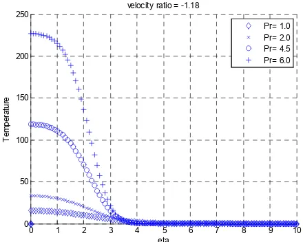
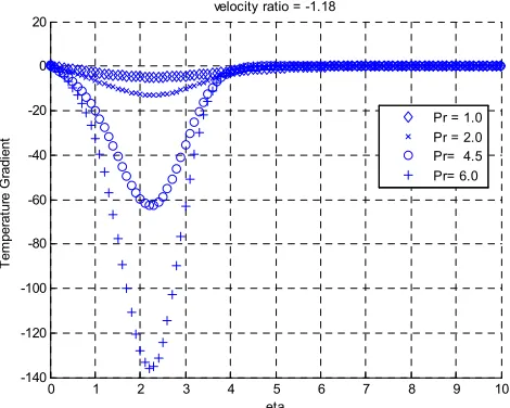
The effects of Prandtl number, negative and positive velocity ratios for an isothermal left side boundary condition on the temperature and temperature gradient profiles are illustrated in Figs (3-6). For Fig. 3, each temperature profile, initially decreases and then ultimately goes to zero for large values of η. The temperature gradient profiles for Fig. 4 exhibit an initial decrease in gradient, then a rise followed by an asymptotic approach to zero for all the profiles. Based on these observations, it is worthwhile to note that considering the values of Prandtl numbers, if the momentum diffusivity is high (i.e. free movement of fluid due to density differences) and the thermal diffusivity is low (i.e. for low thermal conductivity fluids), the overall heat transfer is facilitated by natural convection. Prandtl number is relatively high for such cases. This is what obtains for natural convection of certain fluids, for example water.

Figure 3. Temperature distributions for zero flux, negative velocity ratio, different values of Prandtl number.

0 0.5 1 1.5 2 2.5

0 0.5 1 1.5 2 2.5 3 3.5 4 4.5 5

eta

D

e

p

e

n

d

e

n

t

V

a

ri

a

b

le

s

Stagnation Point Flow

f df/deta d2f/deta2 pressure

0 1 2 3 4 5 6 7 8 9 10 0

50 100 150 200 250

velocity ratio = -1.18

T

e

m

p

e

ra

tu

re

eta

Figure 4. Temperature gradient profiles for zero flux, negative velocity ratio, different values of Prandtl number.

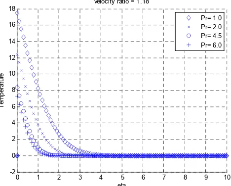
Figure 5. Temperature profiles for zero flux, positive velocity ratio, different values of Prandtl number.

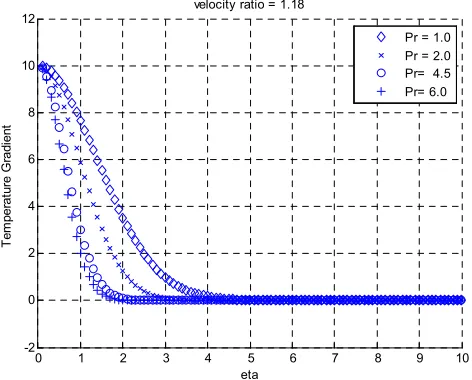
Figure 6. Temperature gradient profiles for zero flux, positive velocity ratio, different values of Prandtl number.

The impact of a positive velocity ratio on the temperature and temperature gradient profiles can be seen in Fig. 5 and Fig. 6. As expected, both the temperature and the temperature gradient decrease along the surface in accordance with the specified boundary condition. But the positive velocity ratio effect on the zero flux boundary condition is profound. This is as a result of a significant drop in temperature and the alteration of the shape of the boundary layer. Hence an increase in the velocity ratio causes the temperature of the fluid to decrease. For such a case, the thickness of the thermal boundary layer decreases due to the fluid at the surface having a temperature lower than that of the flat plate.

Figure 7. Temperature distributions for unit positive flux, negative velocity ratio, different values of Prandtl number.

Figure 8. Temperature gradient distributions for unit positive flux, negative velocity ratio, different values of Prandtl number.

Figs. 7 and 8 show the profiles resulting from specifying a unit positive flux at the left boundary of the plate as well as a negative velocity ratio. The profiles have the same shapes as those for the zero flux except that their magnitudes are different. The temperature profiles display a steeper front and higher magnitude in this case. The temperature gradients are

0 1 2 3 4 5 6 7 8 9 10

-140 -120 -100 -80 -60 -40 -20 0 20

velocity ratio = -1.18

T

e

m

p

e

ra

tu

re

G

ra

d

ie

n

t

eta

Pr = 1.0 Pr = 2.0 Pr= 4.5 Pr= 6.0

0 1 2 3 4 5 6 7 8 9 10

-0.02 0 0.02 0.04 0.06 0.08 0.1 0.12 0.14 0.16

velocity ratio = 1.18

T

e

m

p

e

ra

tu

re

eta

Pr= 1.0 Pr= 2.0 Pr= 4.5 Pr= 6.0

0 1 2 3 4 5 6 7 8 9 10

-0.2 -0.15 -0.1 -0.05 0 0.05

velocity ratio = 1.18

T

e

m

p

e

ra

tu

re

G

ra

d

ie

n

t

eta

Pr = 1.0 Pr = 2.0 Pr= 4.5 Pr= 6.0

0 1 2 3 4 5 6 7 8 9 10

0 50 100 150 200 250 300 350 400 450

velocity ratio = -1.18

T

e

m

p

e

ra

tu

re

eta

Pr= 1.0 Pr= 2.0 Pr= 4.5 Pr= 6.0

0 1 2 3 4 5 6 7 8 9 10

-250 -200 -150 -100 -50 0

velocity ratio = -1.18

T

e

m

p

e

ra

tu

re

G

ra

d

ie

n

t

eta

also more prominent. With regards to the magnitudes of the scalar profiles and the assigned values of the Prandtl number, we note that if the momentum diffusivity is low (i.e. there is not enough density differences to enhance the movement of the fluid) and the thermal diffusivity is low (i.e. for fluids with low values of thermal diffusivity), then the transfer of heat from the from the boundary will not be facilitated as the fluid is not only incapable of absorbing heat but also cannot move freely due to insufficient momentum from convection currents. The profiles we encounter here are better assessed if we compare Figs. 7 and 3 to see how the introduction of a positive flux at the left boundary (with all the other parameters remaining the same) results in an overall relative increase in temperature within this region. It is obvious that we encounter a vector quantity here whose direction informs us that heat is drawn out of the plate.

Figs 9 and 10 show the effect of a positive velocity ratio on the temperature and flux profiles. An increase in velocity ratio results in a significant temperature loss implying that the thermal boundary layer decreases. Again it should be remembered that because of its dependence on the fluid velocity, the temperature field is affected by the velocity ratio. As the velocity ratio increases, the temperature of the fluid decreases. This is because the positive value of the velocity ratio promotes heat transfer to the fluid. Fig. 10 shows a monotonic rise in temperature gradient until it gets to a point where the temperatures of all the fluids become zero in agreement with the specified Dirichlet boundary condition at the right end of the plate.

Figure 9. Temperature distributions for unit positive flux, positive velocity ratio, Prandtl numbers.

Figs 11 and 7 illustrate the effect of changing the sign and hence the direction of the flux at the left boundary for the same problem parameters. One should not loose sight of the Fourier’s law and the implication of its vector interpretation concerning the direction of the flux. Consequently Fig. 7 records a much higher temperature than Fig. 11. However Fig. 11 displays much steeper slopes than Fig. 7. Fig. 12 gives values of the flux and reflects the heat transfer trend of

Fig. 11.

Fig. 13 displays the temperature profiles for a unit negative flux specification at the left boundary, keeping the magnitude of the velocity ratio the same. This gives us a handle on the magnitude of heat flow as well as the direction. A comparison made between Figs 13 and 9 yields valuable information concerning the link between the temperature profiles displayed in each case as well as magnitude and signs (directions) of the flux specification. Figs 10 and 14 give further information concerning the flux. While Fig. 9 shows a monotonic decrease in temperature for all values of Prandtl number, Fig. 13 displays an exactly opposite trend. Each of these cases is in consonance with the vector interpretation of the Fourier’s law. However, one thing they both have in common is that at the regionη>3 all the profiles move towards satisfying the Dirichlet boundary condition specification at the right boundary.

Figure 10. Temperature gradient distributions for unit positive flux, positive velocity ratio, Prandtl numbers.

Figure 11. Temperature distributions for unit negative flux, negative velocity ratio, Prandtl numbers.

0 1 2 3 4 5 6 7 8 9 10

-2 0 2 4 6 8 10 12 14 16 18

velocity ratio = 1.18

T

e

m

p

e

ra

tu

re

eta

Pr= 1.0 Pr= 2.0 Pr= 4.5 Pr= 6.0

0 1 2 3 4 5 6 7 8 9 10

-12 -10 -8 -6 -4 -2 0 2

velocity ratio = 1.18

Te

m

p

e

ra

tu

re

G

ra

d

ie

n

t

eta

Pr = 1.0 Pr = 2.0 Pr= 4.5 Pr= 6.0

0 1 2 3 4 5 6 7 8 9 10

-40 -30 -20 -10 0 10 20 30 40 50

velocity ratio = -1.18

T

e

m

p

e

ra

tu

re

eta

Figure 12. Temperature gradient profiles for unit negative flux, negative velocity ratio, Prandtl numbers.

Figure 13. Temperature profiles for unit negative flux, positive velocity ratio, Prandtl numbers.

Figure 14. Temperature gradient profiles for unit negative flux, positive velocity ratio, Prandtl numbers.

5. Conclusions

In this work, we have presented unsteady numerical formulations for stagnation point flow towards a sheet with prescribed surface heat flux and viscous dissipation. Since more emphasis is devoted to the energy component of the formulation, several graphical plots are made to illustrate the temperature and the temperature gradient fields. The numerical results obtained are graphically displayed and discussed for various problem parameters considered in the problem formulation. Numerical experiments involving flux variations are made on the left of the problem domain. For each of these results, we can observe that as we move far from the sheet, the effects of viscous dissipation vanish and the profiles intersect each other at some point.

Some of the basic features of this model can be applied to study a variety of scenarios involving more complex formulations such as heat characteristics for Newtonian and non-Newtonian fluids, flows in porous media and MHD slip flow to mention just a few.

Acknowledgement

We thank the anonymous referee for his/her useful comments.

References

[1] A. Bejan, Convective heat transfer 2nd ed. Wiley NY 1995. [2] K. Hiemenz, “Die grenschicht an einem in den

gleichformingen flussgkeitsstrom eingetauchten ger-aden kreiszylinder, Dingl.”, Polytech. Journal vol. 32 pp. 321-410, 1911.

[3] F. Homann, “Der einfluss grosset zahigkeit bei der stromung um den Zylinder and um die kugel”, Zeitschrift fur Angewandte Mathematic und mechanic, vol. 16 pp. 153-164, 1936.

[4] T. Y. Na Computational methods in engineering boundary value problem, Academic Press, NY 1979.

[5] L. J. Crane, “Flow past a stretching sheet”, Zeitschrift fur Angewandte Mathematik und Physik vol. 21 pp. 645-647, 1970.

[6] P. Caragher and L. J. Crane, “Heat transfer n a continuous stretching sheet”, ZAMM vol. 62 pp. 564-577, 1985.

[7] P. S. Gupta and A. S. Gupta, “Heat and mass transfer for a stretching sheet with uniform suction and blowing”, The Canadian Journal of Chemical Engineering, vol. 55 pp. 744-746, 1977.

[8] T. C. Chiam, “Stagnation point flow towards a stretching sheet” J. Phys. Soc. Jpn. Vol. 63 pp. 2443-2455, 1994. [9] B. C. Sakiadis, “Boundary-layer behavior on continuous solid

surfaces: I. Boundary-layer equations for two-dimensional and axisymmetric flow”, American institute of chemical engineers(AICHE) Journal vol. 7(1) pp. 26-28, 1961.

0 1 2 3 4 5 6 7 8 9 10

-30 -25 -20 -15 -10 -5 0 5 10 15

velocity ratio = -1.18

Te

m

p

e

ra

tu

re

G

ra

d

ie

n

t

eta

Pr = 1.0 Pr = 2.0 Pr= 4.5 Pr= 6.0

0 1 2 3 4 5 6 7 8 9 10

-18 -16 -14 -12 -10 -8 -6 -4 -2 0 2

velocity ratio = 1.18

T

e

m

p

e

ra

tu

re

eta

Pr= 1.0 Pr= 2.0 Pr= 4.5 Pr= 6.0

0 1 2 3 4 5 6 7 8 9 10

-2 0 2 4 6 8 10 12

velocity ratio = 1.18

T

e

m

p

e

ra

tu

re

G

ra

d

ie

n

t

eta

[10] B. C. Sakiadis, “Boundary –layer behavior on continuous solid surfaces: II The boundary layer on a continuous flat surface”, AICHE J. vol. 7 pp. 221-225, 1961. Doi:10.1002/aic.690070211

[11] T. R. Mahapatra and A. S. Gupta, “Heat transfer in stagnation-point flow towards a stretching sheet”, Heat and Mass Transfer, vol. 38 pp. 517-521, 2002.

[12] P. Dulal and P. S. Hiremath, “Computational modelling of heat transfer over an unsteady stretching surface embedded in porous medium”, Mecccanica, vol. 45 pp. 415-524, 2009. [13] D. B. Ingham and I. Pop, Transport in porous media III

Elsevier, Oxford 2005.

[14] D. A. Nield and A. Bejan, Convection in porous media, 3rd ed. Springer science and business media inc. N. York 2005. [15] B. K. Dutta, P. Roy A. S. Gupta,” Temperature field in flow

over a stretching sheet with uniform heat flux”, Int. Comm. Heat and Mass Trans vol.28 pp. 1234-1237, 1985.

[16] M. E. Ali and E. Magyari, “Unstaedy fluid and heat flow induced by a submerged stretching surface while its steady motion is slowing down gradually”, Int. Jnl. Heat and Mass Trans. vol. 50 pp. 188-195, 2007.

[17] A. Ishak, R. Nazar, and I. Pop, “Magnetohydrodynamics stagnation point flow towards a stretching vertical sheet”, Magneto-hydrodynamics, vol. 42 pp.17-30, 2006.

[18] H. I. Anderson, “MHD flow of viscoelastic fluid past a stretching surface”, Acta Mechanica,, vol. 95 pp. 227-230, 1992.

[19] M. I. Char, “Heat and mass transfer in a hydromagnetic flow of the viscoelstic fluid past a stretching surface”, Physics of Fluids vol. 27 pp. 1915-1917, 1994.

[20] T. R. Mahapatra and S. K. Nandy, “Momentum and heat transfer in MHD axisymmetric stagnation point flow over a shrinking sheet”, Jnl. Applied Fluid Mechanics, vol. 6 pp. 121-129, 2011.

[21] O. D. Makinde and W. M. Charles, “Computational dynamics of hydromagnetic stagnation flow towards a stretching sheet”, Applied, Comput. Math. vol. 9 (2010) pp. 243-251, 2010 [22] O. D. Makinde, “On MHD boundary –layer flow and mass

transfer past a vertical plate in a porous medium with constant heat flux”, Int. Jnl. Num. Mthds. For Heat and Fluid flow. Vol. 19 pp. 546-554, 2009.

[23] K. Bhattacharyyya, “Heat transfer in boundary layer stagnation –point flow towards a shrinking sheet with non-uniform heat flux:”, Chin. Physics B vol. 222 pp. 07405-1-07405-5, 2013.

[24] I. Mealey and J. H. Merkin, “Free convection boundary layers on a verical surface in a heat generating porous medium”, IMA Journal of Applied Mathematics vol. 73 pp. 231-253, 2008.

[25] A. Postelnicu and I. Pop, “Similarity solution of free convection boundary layers over vertical and horizontal surfaces in porous media with internal heat generation”, Int. Comm. Heat and Mass Transfer, vol. 26 pp. 1183-1191, 1999. [26] D. C. Wilcox, Basic fluid mechanics 2nd ed. DCW industries