PAC-Bayes Bounds with Data Dependent Priors
Emilio Parrado-Hern´andez EMIPAR@TSC.UC3M.ES
Department of Signal Processing and Communications University Carlos III of Madrid
Legan´es, 28911, Spain
Amiran Ambroladze A.AMBROLADZE@FREEUNI.EDU.GE
Department of Mathematics and Computer Science Tbilisi Free University
Bedia Street
0182 Tbilisi, Georgia
John Shawe-Taylor J.SHAWE-TAYLOR@CS.UCL.AC.UK
Department of Computer Science University College London London, WC1E 6BT, UK
Shiliang Sun SHILIANGSUN@GMAIL.COM
Department of Computer Science and Technology East China Normal University
500 Dongchuan Road Shanghai 200241, China
Editor:Gabor Lugosi
Abstract
This paper presents the prior PAC-Bayes bound and explores its capabilities as a tool to provide tight predictions of SVMs’ generalization. The computation of the bound involves estimating a prior of the distribution of classifiers from the available data, and then manipulating this prior in the usual PAC-Bayes generalization bound. We explore two alternatives: to learn the prior from a separate data set, or to consider an expectation prior that does not need this separate data set. The prior PAC-Bayes bound motivates two SVM-like classification algorithms, prior SVM andη -prior SVM, whose regularization term pushes towards the minimization of the -prior PAC-Bayes bound. The experimental work illustrates that the new bounds can be significantly tighter than the original PAC-Bayes bound when applied to SVMs, and among them the combination of the prior PAC-Bayes bound and the prior SVM algorithm gives the tightest bound.
Keywords: PAC-Bayes bound, support vector machine, generalization capability prediction, clas-sification
1. Introduction
on the training examples. For this reason there has been considerable interest in bounding the generalization in terms of the margin.
In fact, a main drawback that restrains engineers from using these advanced machine learning techniques is the lack of reliable predictions of generalization, especially in what concerns worst-case performance. In this sense, the widely used cross-validation generalization measures indicate little about the worst-case performance of the algorithms. The error of the classifier on a set of sam-ples follows a binomial distribution whose mean is the true error of the classifier. Cross-validation is a sample mean estimation of the true error, and worst-case performance estimations concern the estimation of the tail of the error distribution. One could then employ statistical learning the-ory (SLT) tools to bound the tail of the distribution of errors. Early bounds have relied on covering number computations (Shawe-Taylor et al., 1998; Zhang, 2002), while later bounds have considered Rademacher complexity (Bartlett and Mendelson, 2002). The tightest bounds for practical appli-cations appear to be the PAC-Bayes bound (McAllester, 1999; Langford and Shawe-Taylor, 2002; Catoni, 2007) and in particular the form given in Seeger (2002), Langford (2005) and Germain et al. (2009). However, there still exist a remarkable gap between SLT predictions and practitioners’ ex-periences: SLT predictions are too pessimistic when compared to the actual results data analysts get when they apply machine learning algorithms to real-world problems.
Another issue affected by the ability to predict the generalization capability of a classifier is the selection of the hyperparameters that define the training. In the SVM case, these parameters are the trade-off between maximum margin and minimum training error,C, and the kernel param-eters. Again, the more standard method of cross-validation has proved to be more reliable in most experiments, despite the fact that it is statistically poorly justified and relatively expensive.
The aim of this paper is to investigate whether the PAC-Bayes bound can be tightened towards less pessimistic predictions of generalization. Another objective is to study the implications of the bound in the training of the classifiers. We specifically address the use of the bound in the model selection stage and in the design of regularization terms other than the maximization of the margin. The PAC-Bayes bound (retrospected in Section 2) uses a Gaussian prior centered at the origin in the weight space. The key to the new bounds introduced here is to use part of the training set to compute a more informative prior and then compute the bound on the remainder of the examples relative to this prior. This generalisation of the bound, called prior PAC-Bayes bound, is derived in Section 3. The prior PAC-Bayes bound was initially presented by Ambroladze et al. (2007). A slight nuisance of the prior PAC-Bayes bound is that a separate data set should be available in order to fix the prior. In Section 3.2, we further develop the expectation-prior PAC-Bayes bound as an interesting new approach which does not require the existence of the separate data set. We also derive a PAC-Bayes bound with a non-spherical Gaussian prior. To the best of our knowledge this is the first such application for SVMs.
4.2 presents a second algorithm, namedη-prior SVM as a variant of prior SVMs where the position of component of the prior that goes into the overall classifier is optimised in a continuous range (not picked from a fixed set). Therefore,η-prior SVMs include a first optimization where the direction of the prior is learnt from a separate set of training patterns, and a second optimization that deter-mines (i) the exact position of the prior along the already learnt direction and (ii) the position of the posterior. Furthermore we show that the performance of the algorithm can be bounded rigorously using PAC-Bayes techniques.
In Section 5 the new bounds and algorithms are evaluated on multiple classification tasks after a parameter selection. The experiments illustrate the capabilities of the prior PAC-Bayes bound to provide tighter predictions of the generalisation of an SVM. Moreover, the combination of the new bounds and the two prior SVM algorithms yields more dramatic tightenings of the bound. Besides, these classifiers achieve good accuracies, comparable to those obtained by an SVM with its parameters fixed with ten fold cross validation. We finish the experimental work showing that the use of a different value ofCfor the prior and the posterior that form the (η)prior SVM lead to a further tightening of the bound.
Finally, the main conclusions of this work and some related ongoing research are outlined in Section 6.
2. PAC-Bayes Bound for SVMs
This section is devoted to a brief review of the PAC-Bayes bound theorem of Langford (2005). Let us consider a distribution
D
of patternsxlying in a certain input spaceX
and their corresponding output labelsy(y∈ {−1,1}). SupposeQis a posterior distribution over the classifiersc. For every classifierc, the following two error measures are defined:Definition 1 (True error) The true error cD of a classifier c is defined to be the probability of
misclassifying a pattern-label pair (x,y) selected at random from
D
cD≡Pr(x,y)∼D(c(x)6=y).
Definition 2 (Empirical error)The empirical errorcˆS of a classifier c on a sample S of size m is defined to be the error rate on S
ˆ
cS≡Pr(x,y)∼S(c(x)6=y) = 1 m
m
∑
i=1
I(c(xi)6=yi),
where I(·)is an indicator function equal to1if the argument is true and equal to0if the argument is false.
Now we define two error measures on the distribution of classifiers: the average true error, QD ≡Ec∼QcD, as the probability of misclassifying an instancexchosen uniformly from
D
with aclassifiercchosen according toQ; and the average empirical error ˆQS≡Ec∼QcˆS, as the probability of classifiercchosen according toQmisclassifying an instancexchosen from a sampleS.
Theorem 3 (PAC-Bayes bound)For all prior distributions P(c)over the classifiers c, and for any
δ∈(0,1],
PrS∼Dm ∀Q(c):KL+(QˆS||QD)≤
KL(Q(c)||P(c)) +ln(m+δ1)
m
!
≥1−δ,
where KL(Q(c)||P(c)) =Ec∼QlnQP((cc))is the Kullback-Leibler divergence, and KL+(q||p) =qlnqp+
(1−q)ln11−−qp for p>q and0otherwise.
The proof of the theorem can be found in Langford (2005).
This bound can be specialized to the case of linear threshold classifiers. Suppose themtraining examples define a linear classifier that can be represented by the following equation:
cu(x) =sign(uTφ(x)), (1)
whereφ(x)is a nonlinear projection to a certain feature space1where the linear classification actu-ally takes place, and vectoruin the feature space determines the separating hyperplane. Since we are considering only classifiers with threshold set to zero all the classifiers in the paper can be rep-resented with unit vectors (kwk=1). However, as we will be considering distributions of classifiers we use the notationuto indicate weight vectors that can also be non-unit.
For any unit vector w we can define a stochastic classifier in the following way: we choose the distributionQ(cu) =Q(cu|w,µ), whereu∼
N
(µw,I)is drawn from a spherical Gaussian with identity covariance matrix centered along the direction pointed bywat a distanceµfrom the origin. Moreover, we can choose the priorcu:u∼N
(0,I)to be a spherical Gaussian with identity covari-ance matrix centered at the origin. Then, for classifiers of the form in Equation (1) the generalization performance can be bounded asCorollary 4 (PAC-Bayes bound for SVMs (Langford, 2005))For all distributions
D
, for all δ∈ (0,1], we havePrS∼Dm ∀w,µ:KL+(QˆS(w,µ)||QD(w,µ))≤
µ2
2 +ln(
m+1
δ ) m
!
≥1−δ.
It can be shown (see Langford, 2005) that
ˆ
QS(w,µ) =Em[F˜(µγ(x,y))], (2)
where Em is the average over the m training examples, γ(x,y) is the normalized margin of the training examples
γ(x,y) =yw
Tφ(x)
kφ(x)k , (3)
and ˜F=1−FwhereF is the cumulative normal distribution
F(x) =
Z x
−∞ 1
√
2πe −x2/2
dx. (4)
Note that the SVM expressed as (1) is computed with a single unit vectorw. The generalization error of such a classifier can be bounded by at most twice the average true errorQD(w,µ)of the
corresponding stochastic classifier involved in Corollary 4 (Langford and Shawe-Taylor, 2002). That is, for allµwe have
Pr(x,y)∼D sign(wTφ(x))6=y
≤2QD(w,µ). (5)
3. Data Dependent Prior PAC-Bayes Bounds for SVMs
This section presents some versions of the PAC-Bayes bound that aim at yielding a tighter predic-tion of the true generalizapredic-tion error of the classifier. These new bounds introduce more sophisticated designs for the prior distribution over the classifiers in order to reduce its divergence with the pos-terior distribution. The first set of bounds learns the prior distribution from a separate training data set that will not be used in the computation of the bound, whilst the second set learns the prior from mathematical expectations, avoiding to leave out a subset of patterns to calculate the bound.
3.1 Bounds Based on a Separate Set of Training Data
This section is a further extension of previous ideas presented by Ambroladze et al. (2007).
Our first contribution is motivated by the fact that the PAC-Bayes bound allows us to choose the prior distribution, P(c). In the standard application of the boundP(c)is chosen to be a spherical Gaussian centered at the origin. We now consider learning a different prior based on training an SVM on a subsetT of the training set comprisingrtraining patterns and labels. In the experiments this is taken as a random subset, but for simplicity of the presentation we will assumeT comprises the lastrexamples{xk,yk}mk=m−r+1.
With theser examples we can learn an (unit and biased) SVM classifier,wr, and form a prior P(wr,η)∼
N
(ηwr,I)consisting of a Gaussian distribution with identity covariance matrix centered alongwrat a distanceηfrom the origin.The introduction of this priorP(wr,η)in Theorem 3 results in the following new bound.
Corollary 5 (Single-prior PAC-Bayes bound for SVMs)Let us consider a prior on the distribution of classifiers consisting of a spherical Gaussian with identity covariance centered along the direc-tion given bywrat a distanceηfrom the origin. Classifierwr has been learnt from a subset T of r examples a priori separated from a training set S of m samples. Then, for all distributions
D
, for allδ∈(0,1], we havePrS∼Dm ∀wm,µ:KL+(QˆS\T||QD)≤
||ηwr−µwm||2
2 +ln(
m−r+1
δ ) m−r
!
≥1−δ,
whereQˆS\T is a stochastic measure of the empirical error of the classifier on the m−r samples not used to learn the prior. This stochastic error is computed as in Equation (2) but averaged over S\T .
Using a standard expression for the KL divergence between two Gaussians in anNdimensional space,
KL(N(µ0,Σ0)k
N
(µ1,Σ1)) =1 2
ln
detΣ1
detΣ0
+tr(Σ−1
1 Σ0) + (µ1−µ0)
TΣ−1
1 (µ1−µ0)−N
, (6)
the KL divergence between prior and posterior is computed as follows:
KL(Q(w,µ)||P(wr,η)) =KL(N(µw,I)k
N
(ηwr,I)) = 12||µw−ηwr||
2.
Intuitively, if the selection of the prior is appropriate, the bound can be tighter than the one given in Corollary 4 when applied to the SVM weight vector on the whole training set. It is worth stressing that the bound holds for allwand so can be applied to the SVM trained on the whole set. This might at first appear to be ‘cheating’, but the critical point is that the bound is evaluated on the setS\T not involved in generating the prior. The experimental work illustrates how in fact this bound can be tighter than the standard PAC-Bayes bound.
Moreover, the structure of the prior may be further refined in exchange for a very small increase in the penalty term. This can be achieved with the application of the following result.
Theorem 6 (Mixture prior PAC-Bayes bound) Let
P
(c) =∑Jj=1πjPj(c) be a prior distribution over classifiers consisting of a mixture of J components{Pj(c)}Jj=1combined with positive weights {πj}Jj=1so that∑Jj=1πj=1. Then, for allδ∈(0,1],PrS∼Dm ∀Q(c):KL+(QˆS||QD)≤min
j
KL(Q(c)||Pj(c)) +lnm+δ1+lnπj1 m
!
≥1−δ.
Proof
The bound in Theorem 3 can be instantiated for the ensemble prior
P
(c)PrS∼Dm ∀Q(c): KL+(QˆS||QD)≤
KL(Q(c)||
P
(c)) +ln(m+1δ ) m
!
≥1−δ.
We now bound the KL divergence between the posteriorQ(c)and the ensemble prior
P
(c). For any 1≤i≤J:KL(Q(c)k
P
(c)) =Z
c∈CQ(c) lnQ(c)−ln(
J
∑
j=1
πjPj(c)) !
dc
≤
Z
c∈C
Q(c)(lnQ(c)−ln(πiPi(c)))dc=KL(Q(c)kPi(c))−ln(πi),
proof.
Note that the inequality in the proof upper bounds the KL divergence to give a bound equivalent to performing a union bound. In particular applications it may be possible to obtain tighter bounds by estimating this KL divergence more closely.
This result can be also specialized for the case of SVM classifiers. The mixture prior is con-structed by allocating Gaussian distributions with identity covariance matrix along the direction given bywrat distances{ηj}Jj=1from the origin where{ηj}Jj=1are positive real numbers. In such
a case, we obtain
Corollary 7 (Gaussian Mixture-prior PAC-Bayes bound for SVMs) Let us consider a prior dis-tribution of classifiers formed by an ensemble of equiprobable spherical Gaussian disdis-tributions
{Pj(c|wr,ηj)}Jj=1 with identity covariance and meanηjwr, where{ηj}Jj=1 are positive real
num-bers and wr is a linear classifier trained using a subset T of r samples a priori separated from a training set S of m samples. Then, for all distributions
D
, for all posteriors (w,µ) and for allδ∈(0,1], we have that with probability greater than1−δ over all the training sets S of size m sampled from
D
KL+(QˆS\T(w,µ)||QD(w,µ))≤min
j
||ηjwr−µw||2
2 +ln(
m−r+1
δ ) +lnJ
m−r .
Proof The proof is straightforward and can be completed by substituting 1/Jfor allπjin Theorem 6 and computing the KL divergence between prior and posterior as in the proof of Corollary 5.
Note that the{ηj}Jj=1must be chosen before we actually compute the posterior. A linear search
can be implemented for the value ofµthat leads to the tightest bound for each particular prior. In the case of a mixture prior, the search is repeated for every member of the ensemble and the reported value of the bound is the tightest one found during the searches.
Moreover, the data distribution can also shape the covariance matrix of the Gaussian prior. Rather than take a spherically symmetric prior distribution we choose the variance in the direction of the prior vector to beτ>1. As with the prior PAC-Bayes bound the mean of the prior distribution is also shifted from the original in the directionwr. Seeger (2002) has previously considered non-spherical priors and (different) non-non-spherical posteriors in bounding Gaussian process classification. Our application to SVMs is not restricted to using specific priors and posteriors so that we have the flexibility to adapt our distributions in order to accommodate the prior derived from the last part of the data.
We introduce notation for the norms of projections for unit vectoru,Puk(v) =hu,viandPu⊥(v)2=
kvk2−Pk
u(v)2.
Theorem 8 (τ-prior PAC-Bayes bound for linear classifiers) Let us consider a prior P(c|wr,τ,η) distribution of classifiers consisting of a Gaussian distribution centred onηwr, with identity covari-ance matrix in all directions exceptwr in which the variance isτ2. Then, for all distributions
D
, for allδ∈(0,1], we have that with probability at least1−δover all the training samples of size m drawn fromD
, for all posterior parameters (w, µ),(ln(τ2) +τ−2−1+Pk
wr(µw−ηwr)
2/τ2+P⊥
wr(µw)
2) +2 ln(m−r+1
δ )
2(m−r) .
Proof The application of the PAC-Bayes theorem follows that of Langford (2005) except that we must recompute the KL divergence. Using the expression for the KL divergence between two Gaussian distributions of (6) we obtain
KL(Q(w,µ)kP(wr,τ,η)) =
1 2 ln(τ
2) +
1
τ2−1
+P k
wr(µw−ηwr)
2
τ2 +Pw⊥r(µw)
2
!
,
and the result follows.
Note that the quantity
ˆ
QS\T(w,µ) =Em−r[F˜(µγ(x,y))]
remains unchanged as the posterior distribution is still a spherical Gaussian centred atw.
3.2 Expectation-Prior PAC-Bayes Bound for SVMs
In this section, we attempt to start an interesting new approach on exploiting priors without the aid of a separate data set. The basic idea is to adopt the mathematical expectation of some quantity and then approximate this expectation by an empirical average computed on the available data.
An expectation that may result in reasonable priors is E(x,y)∼D[yφ(x)], which is used in the
derivation of the bound below. Definewp=E(x,y)∼D[yφ(x)]wherey∈ {+1,−1}. A special case
ofwp is 12(w+−w−)withw+=E(x,y)∼D,y=+1[φ(x)],w−=E(x,y)∼D,y=−1[φ(x)]when each class
has the same prior probability. We use its general form in deriving bounds.
Given a sample set S including m examples, the empirical estimate of wp would be ˆwp =
E(x,y)∼S[yφ(x)] = m1∑ m
i=1[yiφ(xi)]. We have the following bound.
Theorem 9 (Single-expectation-prior PAC-Bayes bound for SVMs) For all
D
, for all Gaussian prior P∼N
(ηwp,I)over margin classifiers, for allδ∈(0,1]:PrS∼Dm (∀w,µ:KL+(QˆS(w,µ)||QD(w,µ))≤
1
2(kµw−ηwˆpk+η
R
√m(2+q2 ln2δ))2+ln(2(m+1)
δ )
m )≥1−δ,
where the posterior is Q∼
N
(µw,I)with R=supxkφ(x)k.Proof First, we try to boundKL(Q||P). We have
KL(Q||P) = 1
2kµw−ηwpk
2
= 1
2kµw−ηwˆp+ηwˆp−ηwpk
2
= 1
2kµw−ηwˆpk
2+1
2kηwˆp−ηwpk
2+ (µw
−ηwˆp)⊤(ηwˆp−ηwp)
≤ 12kµw−ηwˆpk2+ 1 2η
2
where the last inequality uses Cauchy-Schwarz inequality. Now it suffices to boundkwˆp−wpk. DefineR=supxkφ(x)k. It is simple to show that sup(x,y)kyφ(x)k=supxkφ(x)k=R. With reference to a result on estimating the center of mass (Shawe-Taylor and Cristianini, 2004), we have
Pr
kwˆp−wpk ≥ 2R
√
m+ε
≤exp
−2mε 2
4R2
.
Setting the right hand side equal toδ/2, solving forεshows that with probability at least 1−δ/2, we have
kwˆp−wpk ≤ R
√
m 2+
r
2 ln2
δ
!
. (8)
Defineb=√R m
2+q2 ln2δ, we have
PrS∼Dm
KL(Q||P)≤1
2kµw−ηwˆpk
2+1
2η
2b2+ηbkµw−ηwˆ
pk
≥1−δ/2. (9)
Then, according to Theorem 3, we have
PrS∼Dm ∀Q(c):KL+(QˆS||QD)≤
KL(Q||P) +ln(2(mδ+1))
m
!
≥1−δ/2. (10)
Definea=kµw−ηwˆpk. Combining (9) and (10), we get
PrS∼Dm ∀w,µ:KL+(QˆS(w,µ)||QD(w,µ))≤
1 2a2+
1
2η2b2+ηab+ln( 2(m+1)
δ ) m
!
≥1−δ,
where we used(1−δ/2)2>1−δ.Rewriting the bound as
PrS∼Dm ∀w,µ:KL+(QˆS(w,µ)||QD(w,µ))≤
1
2(a+ηb)
2+ln(2(m+1) δ ) m
!
≥1−δ
completes the proof.
Considering at the same time Theorem 9 and the mixture-prior PAC-Bayes bound, it is not difficult to reach the following mixture-expectation-prior PAC-Bayes bound for SVMs.
Theorem 10 (Mixture-expectation-prior PAC-Bayes bound for SVMs)For all
D
, for all mixtures of Gaussian priorP
(c) =∑Jj=1πjPj(c)where Pj∼N
(ηjwp,I) (j=1, . . . ,J),πj≥0and∑Jj=1πj=1 over margin classifiers, for allδ∈(0,1]:PrS∼Dm ∀w,µ:KL+(QˆS(w,µ)||QD(w,µ))≤
min j
1
2(kµw−ηjwˆpk+ηj
R
√m(2+
q
2 ln2δ))2+ln(2(m+1)
δ ) +lnπj1 m
≥1−δ,
Moreover, the expectation prior bound can also be extended to the case where the shape of the covariance matrix of the prior is also determined from the training data:
Theorem 11 (τ-Expectation-prior PAC-Bayes bound) Consider a prior distribution P∼
N
(ηwp,I,τ2)of classifiers consisting of a Gaussian distribution centred onηwp, with identity covariance in all directions exceptwpin which the variance isτ2. Then, for all distributionsD
, for allδ∈(0,1], we havePrS∼Dm (∀w,µ:KL+(QˆS(w,µ)||QD(w,µ))≤
1 2(ln(τ
2) +(kµw−ηwˆpk+η√Rm(2+√2 ln2δ))2−µ2+1
τ2 +µ2−1) +ln( 2(m+1)
δ )
m )≥1−δ,
where the posterior is Q∼
N
(µw,I)with R=supxkφ(x)k. We can recover Theorem 9 by takingτ=1.
Proof According to Theorem 8,
KL(Q||P) =1
2
ln(τ2) + 1
τ2−1+
Pwk∗
p(µw−ηwp)
2
τ2 +Pw⊥∗p(µw)
2
,
wherew∗p=wp/kwpk. The last two quantities can be rewritten as
Pwk∗
p(µw−ηwp)
2
τ2 +Pw⊥∗p(µw)
2 = 1
τ2(
w⊤p
kwpk
(µw−ηwp))2+kµwk2−(
w⊤p
kwpk µw)2
= 1
τ2(
w⊤p
kwpk
µw−ηkwpk)2+kµwk2−(
w⊤p
kwpk µw)2
= 1
τ2(η 2
kwpk2−2ηw⊤pµw) +kµwk2
= 1
τ2(kµw−ηwpk 2
− kµwk2) +kµwk2
= 1
τ2(kµw−ηwpk 2
−µ2) +µ2. By Equation (7), we have
kµw−ηwpk2≤ kµw−ηwˆpk2+η2kwˆp−wpk2+2ηkµw−ηwˆpkkwˆp−wpk. By Equation (8), we have with probability at least 1−δ/2
kwˆp−wpk ≤ R
√
m 2+
r
2 ln2
δ
!
.
Witha=kµw−ηwˆpkandb=√Rm
2+
q 2 ln2δ
, we have
PrS∼Dm
KL(Q||P)≤1
2(ln(τ
2) + 1 τ2−1+
a2+η2b2+2ηab−µ2
τ2 +µ
2)
Then, according to Theorem 3, we have
PrS∼Dm(∀Q(c):KL+(QˆS||QD)≤
KL(Q||P) +ln(2(mδ+1))
m )≥1−δ/2. (12)
Combining (11) and (12) results in
PrS∼Dm (∀w,µ:KL+(QˆS(w,µ)||QD(w,µ))≤
1
2(ln(τ2) +
(a+ηb)2 −µ2+1
τ2 +µ2−1) +ln( 2(m+1)
δ )
m )≥1−δ,
which completes the proof.
4. Optimising the Prior PAC-Bayes Bound in the Design of the Classifier
Up to this point we have introduced the prior PAC-Bayes bounds as a means to tighten the origi-nal PAC-Bayes bound (this fact is illustrated in the experiments included in Section 5). The next contribution of this paper consists of the introduction of the optimisation of the prior PAC-Bayes bound into the design of the classifier. The intuition behind this use of the bounds is that classifiers reporting low values for the bound should yield a good generalization capability.
4.1 Prior SVM
The new philosophy is implemented in the prior SVM by replacing the maximization of the margin in the optimization problem defining the original SVM with a term that pushes towards the tighten-ing of the prior PAC-Bayes bound. This subsection introduces the formulation of the new algorithm, a method to determine the classifier by means of off-the-shelf quadratic programming solvers, and a procedure to compute the prior PAC-Bayes bound for these new classifiers.
4.1.1 FORMULATION OF THEPRIORSVMS
As stated before, the design criterion for the prior SVMs involves the minimization of the prior PAC-Bayes bound. Let us consider the simplest case of the bound, that is, a single prior centered on
ηwr, wherewris the unit vector weight of the SVM constructed withrtraining samples andηis a scalar fixed a priori. For simplicity, we assume thesersamples are the last ones in the training set
{(xl,yl)}lm=m−r+1. Therefore,wrcan be expressed in terms of these input patterns as:
wr=
∑ml=m−r+1ylαlφ(xl)
∑ml=m−r+1ylαlφ(xl)
.
In such a case, a small bound on the error of the classifier is the result of a small value ofkηwr− µwk2, and a large value of the normalized margin of Equation (3) for the remaining training
exam-plesγ(xi,yi),i=1, . . . ,m−r.
We start by addressing the separable case. Under perfect separability conditions, a good strategy to obtain a classifier of minimal bound is to solve the following optimization problem:
min w
1
2kw−ηwrk
2
subject to
yiwTφ(xi)≥1 i=1, . . . ,m−r. (14)
Clearly, the objective function of (13) attempts to reduce the value of the right hand side of the bound, while the constraints in (14) that impose the separability of the classes lead to a small ˆQS.
Once w is found through the solution of (13) with constraints (14) the proper bound on the average true error of the prior SVM can be obtained by means of a further tuning ofµ(that is, using µwinstead ofwas mean of the posterior distribution), where this last tuning will not changew.
The extension of the prior SVM to the non-separable case is easily carried out through the introduction of positive slack variables{ξi}mi=−1r. Then the optimization problem becomes
min w,ξi
" 1
2kw−wrk
2+Cm
∑
−ri=1
ξi #
(15)
subject to
yiwTφ(xi)≥1−ξi i=1, . . . ,m−r, (16)
ξi≥0 i=1, . . . ,m−r. (17)
Note that the constraints in (16) also push towards the minimization of the stochastic error ˆ
QS. In this sense, for a samplexon the wrong side of the margin we haveξ=1−ywTφ(x)>1, which leads to a marginγ<0 and thus an increase in ˆQS(see Equations (2) to (4)). Therefore, by penalizingξwe enforce a small ˆQS.
Furthermore, Corollary 7 allows us to use a mixture ofJdistributions instead of one at the cheap cost of lnmJ. This can be used to refine the selection of the weight vector of the prior SVMs through the following procedure:
1. First we determine a unit wr with samples{(xl,yl)}ml=m−r+1. Then we construct a mixture
prior withJ Gaussian components with identity covariance matrices centered atηjwr, with
ηjbeingJ real positive constants.
2. For every element in the mixture we obtain a prior SVM classifierwjsolving
min wj,ξi
" 1 2kw
j
−ηjwrk2+C
m−r
∑
i=1
ξi #
subject to
yiφ(xi)Twj≥1−ξi i=1, . . . ,m−r,
ξi≥0 i=1, . . . ,m−r.
Afterwards, we obtain the boundsQDj corresponding to the average true error of each one of theJprior SVMs by tuningµ(see Corollary 6).
3. We finally select as the prior SVM thewjthat reports the lowest boundQj
D.
It should be pointed out that each prior scaling (ηj) that is tried increases the computational burden of the training of the prior SVMs by an amount corresponding to an SVM problem with m−rdata points.
4.1.2 COMPUTING THEPAC-BAYESBOUND FOR THEPRIORSVMS
The remainder of the section presents a method to compute the PAC-Bayes bound for a prior SVM obtained through the procedure described above. To simplify notation we have introduced the nonunit weight vectorwm−r=w−ηwr, that includes the posterior part of the prior SVM. The bound is based on the relationship between two distributions of classifiers: the priorP(wr,η)∼
N
(ηwr,I) and the posteriorQ(w,µ)∼N
(µw,I).The stochastic error ˆQSin the left hand side of the bound can be straightforwardly obtained by using a unit win (27) in Equations (2) to (4). For the right hand side of the bound, we need to compute KL(Q(w,µ)||P(wr,η)) =kηwr−µwk
2
2 which can be rewritten as
KL(Q(w,µ)||P(wr,η)) = 1
2 µ
2+η2
−2µη(η+wTm−rwr)
.
4.2 η-Prior SVM
When the prior SVM is learnt within a mixture priors setting, the last stage of the optimization is the selection of the best prior-component/posterior pair, among theJ possibilities. These prior-component/posterior pairs are denoted by(ηj,wj), whereηj is the jth scaling of the normalized priorwr. From the point of view of the prior, this selection process can be regarded as a search over the set of scalings using the mixture-prior PAC-Bayes bound as fitness function. Note that the evaluation of such a fitness function involves learning the posterior and the tuning ofµ.
The idea presented in this section actually consists of two turns of the screw. First, the search in the discrete set of priors is cast as a linear search for the optimal scalingηin a continuous range of scalings[η1,ηJ]. Second, this linear search is introduced into the optimization of the posterior. Therefore, instead of optimizing a posterior for every scaling of the prior, the optimal scaling and posterior given a normalized prior are the output of the same optimization problem.
The sequel is devoted to the derivation of the resulting algorithm, called theη-prior SVMs, and to its analysis using the prior PAC-Bayes bound framework.
4.2.1 DERIVATION OF THEη-PRIORSVMS
Theη-prior SVM is designed to solve the following problem:
min v,η,ξi
" 1 2kvk
2+Cm−r
∑
i=1
ξi #
subject to
yi(v+ηwr)Tφ(xi)≥1−ξi i=1, . . . ,m−r,
ξi≥0 i=1, . . . ,m−r.
The final (unit vector) classifier will be
w= (v+ηwr)/kv+ηwrk.
After a derivation analogous to that presented in Appendix A, we arrive at the following quadratic program
max αi
m−r
∑
i=1
αi− 1 2
m−r
∑
i,j=1
subject to
m−r
∑
i=1
m
∑
k=m−r+1
αiyiα˜kykκ(xi,xk) =
m−r
∑
i=1
yiαigi=0 i=1, . . . ,m−r,
0≤αi≤C i=1, . . . ,m−r,
wheregi=∑mk=m−r+1α˜kykκ(xi,xk)and ˜αkare the normalized dual variables for the prior learnt from the lastr samples, {xk}mk=m−r+1. Once we have solved for αi, we can compute ηby considering some jsuch that 0<αj<Cand using the equation
yj
m−r
∑
i=1
αiyiκ(xi,xj) +ηgj !
=1.
4.2.2 BOUNDS FORη-PRIORSVMS
The statistical analysis of theη-prior SVMs can be performed using theτ-prior PAC-Bayes bound of Theorem 8, andτ-expectation prior PAC-Bayes bound. Rather than take a spherically symmetric prior distribution we choose the variance in the direction of the prior vector to beτ2>1. As with the
prior SVM analysis the mean of the prior distribution is also shifted from the origin in the direction wr.
In order to apply the bound we need to consider the range of priors that are needed to cover the data in our application. The experiments conducted in the next section require a range of scalings ofwr from 1 to 100. For this we can choose η=50, τ=50, andµ≤100 in all but one of our experiments, giving an increase in the bound over the factor Pw⊥r(µw)2 directly optimized in the
algorithm of
ln(τ2) +τ−2−1+Pk
wr(µw−ηwr)
2/τ2
2(m−r) ≤
ln(τ) +0.5τ−2
m−r ≈
3.912
m−r. (18)
We include Equation (18) to justify that our algorithm optimises a quantity that is very close to the expression in the bound. Note that the evaluation of the bounds presented in the experimental section are computed using the expression from Theorem 8 and not this approximate upper bound. One could envisage making a sequence of applications of the PAC-Bayes bound with spherical priors using the union bound and applying the result with the nearest prior. This strategy leads to a slightly worse bound as it fails to take into account the correlations between the different priors. This fact is illustrated in Section 5.
5. Experiments
This section is devoted to an experimental analysis of the bounds and algorithms introduced in the paper. The comparison of the algorithms is carried out on classification preceded by model selection tasks using some UCI (Blake and Merz, 1998) data sets (see their description in terms of number of instances, input dimensions and numbers of positive/negative examples in Table 1).
5.1 Experimental Setup
Problem # Examples Input Dim. Pos/Neg
Handwritten-digits (han) 5620 64 2791 / 2829
Waveform (wav) 5000 21 1647 / 3353
Pima (pim) 768 8 268 / 500
Ringnorm (rin) 7400 20 3664 / 3736
Spam (spa) 4601 57 1813 / 2788
Table 1: Description of data sets in terms of number of examples, number of input variables and number of positive/negative examples.
subsets with 20%, 30%, . . ., 100% of the training patterns, in order to analyse the dependence of the bounds with the number of samples used to train the classifier. Note that all the training subsets from the same partition share the same test set.
With each of the training sets we learned a classifier with Gaussian RBF kernels preceded by a model selection. The model selection consists in the determination of an optimal pair of hy-perparameters (C,σ). C is the SVM trade-off between the maximization of the margin and the minimization of the number of misclassified training samples;σis the width of the Gaussian ker-nel,κ(x,y) =exp(−kx−yk2/(2σ2)). The best pair is sought in a 7×5 grid of parameters where
C∈ {0.01,0.1,1,10,100,1000,10000}andσ∈ {1 4
√
d, 1 2
√
d,√d,2√d,4√d},dbeing the input space dimension.
With respect to the parameters needed by the prior PAC-Bayes bounds, the number of priorsJ and the amount of patterns separated to learn the prior, the experiments reported by Ambroladze et al. (2007) suggest thatJ=10 andr=50% of the training set size lead to reasonable results.
The setup to calculate the bound values displayed in the next tables was as follows. We trained an instance of the corresponding classifier for each position of the grid of hyperparameters and compute the bound. We selected for that type of classifier the minimum value of the bound found through the whole grid. Then we averaged the 50 values of the bound corresponding to each of the training/testing partitions. We completed the average with the sample standard deviation. Note that proceeding this way we select a (possibly) different pair of hyperparameters for each of the 50 partitions. That is the reason why we name this task model selection plus classification.
The test error rates are computed after the following procedure. For each one of the training/test partitions we carried out the model selection described in the previous paragraph and selected the classifier of minimum bound. We classified the test set with this classifier and obtain the test error rate for those particular classifier and partition. Then we averaged the 50 test error rates to yield the test error rate for those particular data set, model selection method and type of classifier. Note again that the model selection has a significant impact on the reported test error rates.
5.2 Results and Discussion
The section starts presenting an analysis of the performance of SVM with the prior PAC Bayes bounds introduced in this paper. We show how in most cases the use of an informative prior leads to a significant tightening of the bounds on the true error of the classifier. The analysis is then extended towards the new algorithms prior SVM andη-prior SVM. We show how their true error is predicted more accurately by the prior PAC Bayes bound. The observed test errors achieved by these algorithms are comparable to those obtained by SVMs with their hyperparameters fixed through ten fold cross validation. Finally, the prior SVM framework enables the use of a different value of parameterC for prior and posterior, that can be tuned using the prior PAC Bayes bound. The experiments show that the use of different values ofC contributes to get even tighter lower bounds.
5.2.1 ANALYSIS OF THESVMWITH THEPRIORPAC BAYESBOUNDS
The first set of experiments is devoted to illustrate how tight can be the predictions about the gen-eralisation capabilities of a regular SVM based upon the prior PAC-Bayes bounds. Thus, we have trained SVM using the hyperparameters that arrived at a minimum value of each of the following bounds:
PAC Bayes: the model selection is driven by the PAC Bayes bound of Langford (2005).
Prior PB: model selection driven by the mixture-prior PAC-Bayes bound of Corollary 7 withJ=
10.
τ-prior PB: τ-prior PAC-Bayes bound of Theorem 8 withJ=10 andτ=50.
Eprior PB: expectation-prior PAC-Bayes bound of Theorem 10.
τ-Eprior PB: τ-expectation prior PAC-Bayes bound of Theorem 11.
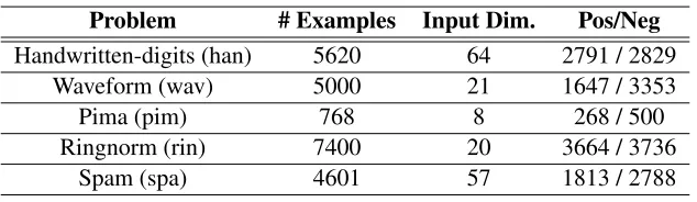
Plots in Figure 1 show the performance of the different bounds as a function of the training set size. All the bounds achieve non trivial results even for training set sizes as small as 16% of the complete data set (20% of the training set). In most of the cases, the bounds with an informative prior are tighter than the original PAC Bayes bound with an spherical prior centred on the origin. The expectation prior is significantly better in data setswav andpim, whilst the prior PAC Bayes and theτ-prior PAC Bayes are the tighter in problemsrinandspa. Table 2 shows the values of the bounds when the SVM is determined using the 100% of the training set (80% of the data).
0.2 0.4 0.6 0.8 1 0.05
0.1 0.15 0.2 0.25 0.3
Me
a
n
o
f
QD
Dataset: han
0.2 0.4 0.6 0.8 1
0.15 0.2 0.25 0.3
Me
a
n
o
f
Q D
Dataset: wav
0.2 0.4 0.6 0.8 1
0.4 0.45 0.5 0.55 0.6 0.65
Me
a
n
o
f
QD
Dataset: pim
0.2 0.4 0.6 0.8 1
0.15 0.2 0.25 0.3 0.35
Me
a
n
o
f
QD
Dataset: spa
Fraction of training set
PAC Bayes Bound on SVM 10 Priors PAC Bayes Bound on SVM
τ Prior PAC Bayes Bound on SVM
10 Priors PAC Bayes Bound on Prior SVM
10 Priors PAC Bayes Bound on ηPrior SVM
τ Prior PAC Bayes Bound on η Prior SVM
0.2 0.4 0.6 0.8 1
0.1 0.2 0.3
Me
a
n
o
f
QD
Dataset: rin
Fraction of training set
Figure 1: Analysis of SVM with data dependent prior PAC Bayes bounds.
Data Set
Bound han wav pim rin spa
PAC Bayes 0.148±0.000 0.190±0.000 0.390±0.001 0.198±0.000 0.230±0.000 Prior PB 0.088±0.004 0.151±0.004 0.411±0.015 0.110±0.004 0.171±0.005 τPrior PB 0.088±0.004 0.152±0.004 0.406±0.013 0.110±0.004 0.172±0.006 EPrior PB 0.107±0.001 0.133±0.001 0.352±0.004 0.194±0.000 0.221±0.001 τEPrior PB 0.149±0.000 0.191±0.000 0.401±0.001 0.199±0.000 0.232±0.000
Table 2: Values of the bounds for SVM.
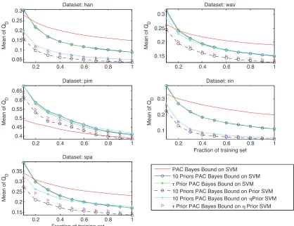
5.2.2 ANALYSIS OFPRIORSVMANDη-PRIORSVM
We repeated the study on the new algorithms, prior SVM andη-prior SVM, which are designed to actually optimise prior PAC-Bayes bounds. The configurations classifier-bound considered for this study were the following:
0.2 0.3 0.4 0.5 0.6 0.7 0.8 0.9 1 0.04
0.06 0.08 0.1 0.12
Me
a
n
o
f
QD
Dataset: han
0.2 0.3 0.4 0.5 0.6 0.7 0.8 0.9 1
0.14 0.16 0.18 0.2 0.22
Me
a
n
o
f
QD
Dataset: wav
0.2 0.3 0.4 0.5 0.6 0.7 0.8 0.9 1
0.35 0.4 0.45 0.5 0.55
Me
a
n
o
f
QD
Dataset: pim
0.2 0.3 0.4 0.5 0.6 0.7 0.8 0.9 1
0.05 0.1 0.15
Me
a
n
o
f
QD
Dataset: rin
Fraction of training set
0.2 0.3 0.4 0.5 0.6 0.7 0.8 0.9 1
0.15 0.2 0.25
Me
a
n
o
f
QD
Dataset: spa
Fraction of training set
10 Priors PAC Bayes Bound on Prior SVM 10 Priors PAC Bayes Bound on ηPrior SVM
τ Prior PAC Bayes Bound on η Prior SVM 10 Priors PAC Bayes Bound on Prior SVM with 2 Cs 10 Priors PAC Bayes Bound on ηPrior SVM with 2 Cs
τ Prior PAC Bayes Bound on η Prior SVM with 2 Cs
Figure 2: Bounds learning a prior classifier.
η-PSVM + Prior PB: η-prior SVM of Section 4.2.1 and mixture-prior PAC-Bayes bound of Corol-lary 7 consideringηcomes from a mixture prior setting ofJ=50 componentsηjwrwith the
ηj equally spaced betweenη1=1 andη50=100. This setting minimizes the penalty term in the prior PAC-Bayes bound as we are not actually using these components to learn the posterior.
η-PSVM +τ-Prior PB: η-prior SVM and the bound in Theorem 8.
As baseline results we include the better bounds found in the analysis of the SVM:
τ-Prior PB: τprior PAC-Bayes bound of Theorem 8 withJ=10 andτ=50.
EPrior PB: expectation-prior PAC-Bayes bound of Theorem 10.
The plots in Figure 2 show the bounds on the true error, QD, for the studied configurations
Data Set
Bound han wav pim rin spa
Prior SVM
Prior PB 0.037±0.004 0.128±0.004 0.386±0.016 0.046±0.003 0.137±0.005 η-Prior SVM
Prior PB 0.050±0.006 0.154±0.004 0.419±0.014 0.053±0.004 0.177±0.006 τPrior PB 0.047±0.005 0.135±0.004 0.397±0.014 0.050±0.004 0.147±0.006
SVM
τPrior PB 0.088±0.004 0.152±0.004 0.406±0.013 0.110±0.004 0.172±0.006 EPrior PB 0.107±0.001 0.133±0.001 0.352±0.004 0.194±0.000 0.221±0.001
Table 3: Values of the bounds on the prior SVM andη-prior SVM classifiers.
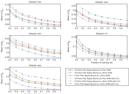
0.2 0.3 0.4 0.5 0.6 0.7 0.8 0.9 1
0.04 0.06 0.08 0.1 0.12
Me
a
n
o
f
QD
Dataset: han
0.2 0.3 0.4 0.5 0.6 0.7 0.8 0.9 1
0.14 0.16 0.18 0.2 0.22
Me
a
n
o
f
QD
Dataset: wav
0.2 0.3 0.4 0.5 0.6 0.7 0.8 0.9 1
0.35 0.4 0.45 0.5 0.55
Me
a
n
o
f
QD
Dataset: pim
0.2 0.3 0.4 0.5 0.6 0.7 0.8 0.9 1
0.05 0.1 0.15
Me
a
n
o
f
QD
Dataset: rin
Fraction of training set
0.2 0.3 0.4 0.5 0.6 0.7 0.8 0.9 1
0.15 0.2 0.25
Me
a
n
o
f
QD
Dataset: spa
Fraction of training set
10 Priors PAC Bayes Bound on Prior SVM 10 Priors PAC Bayes Bound on ηPrior SVM
τ Prior PAC Bayes Bound on η Prior SVM 10 Priors PAC Bayes Bound on Prior SVM with 2 Cs 10 Priors PAC Bayes Bound on ηPrior SVM with 2 Cs
τ Prior PAC Bayes Bound on η Prior SVM with 2 Cs
Figure 3: Bounds when prior and posterior have a different value ofC.
Notice that in most of the configurations where the prior is learnt from a separate set the new bounds achieve a significant cut in the value of the PAC-Bayes bound, which indicates that learning an informative prior distribution helps to tighten the PAC-Bayes bound.
Data Set
Bound han wav pim rin spa
Prior SVM
Prior PB 0.037±0.004 0.128±0.004 0.386±0.016 0.046±0.003 0.137±0.005 Prior PB 2C 0.033±0.002 0.126±0.004 0.341±0.019 0.041±0.002 0.113±0.004
η-Prior SVM
Prior PB 0.050±0.006 0.154±0.004 0.419±0.014 0.053±0.004 0.177±0.006 Prior PB 2C 0.035±0.003 0.154±0.004 0.401±0.018 0.049±0.003 0.150±0.005 τPrior PB 0.047±0.005 0.135±0.004 0.397±0.014 0.050±0.004 0.147±0.006 τPrior PB 2C 0.031±0.002 0.126±0.004 0.345±0.019 0.039±0.002 0.111±0.005
Table 4: Values of the bounds on the prior SVM andη-prior SVM classifiers when different values ofCare used for prior and posterior.
Data Set
Bound han wav pim rin spa
Prior SVM
Prior PB 0.010±0.004 0.086±0.007 0.246±0.034 0.016±0.003 0.082±0.009 Prior PB 2C 0.011±0.003 0.091±0.009 0.251±0.038 0.017±0.003 0.069±0.007
η-Prior SVM
Prior PB 0.010±0.005 0.086±0.006 0.236±0.028 0.016±0.003 0.080±0.009 Prior PB 2C 0.011±0.003 0.087±0.009 0.242±0.039 0.018±0.003 0.068±0.008 τPrior PB 0.010±0.005 0.085±0.006 0.238±0.028 0.016±0.003 0.080±0.009 τPrior PB 2C 0.011±0.003 0.092±0.010 0.248±0.042 0.018±0.003 0.070±0.007
SVM
10 FCV 0.008±0.003 0.087±0.007 0.251±0.023 0.016±0.003 0.067±0.006
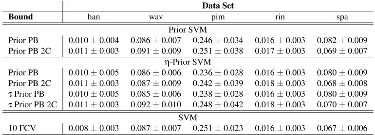
Table 5: Test error rates achieved by prior SVM andη-prior SVM classifiers when the hyperparam-eters are those that minimise a PAC Bayes bound. Prior and posterior are allowed to use a different value of the hyperparameterC.
To evaluate the goodness of this modification, we carried out again the experiments in this subsection but now allowing the prior and posterior to take different values ofC from within the range proposed at the beginning of the section. The results displayed in Figure 3 and Table 4 show that the introduction of a differentCsignificantly reduces the value of the bound.
Finally, Table 5 gives some insight about the performance of the new algorithms in terms of observed test error. The joint analysis of the bounds and the error rates on a separate test set shows that the prior PAC Bayes bounds are achieving predictions on the true error very close to the empir-ical estimations; as an example, for data setwavthe bound onQD is around 13% and the empirical
estimation is around 9%. Moreover, the combination of the new classifiers and bounds perform similarly to an SVM plus ten fold cross validation in terms of accuracy.
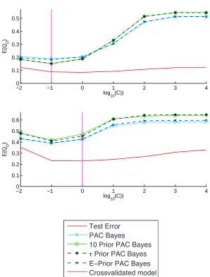
−2 −1 0 1 2 3 4 0
0.1 0.2 0.3 0.4 0.5
log 10(C))
E{Q
D
}
−2 −1 0 1 2 3 4
0 0.1 0.2 0.3 0.4 0.5 0.6
log 10(C))
E{Q
D
}
Test Error PAC Bayes
10 Prior PAC Bayes τ Prior PAC Bayes E−Prior PAC Bayes Crossvalidated model
Figure 4: Values of bounds and observed test error rate as a function ofC for data setswav (top plot) andpim(bottom).
says that high values ofCare likely to result in overfit, since the SVM is keener in reducing the training set error. However, our experiments seem to show that the bounds are overreacting to that behavior.
6. Conclusions
mean and/or covariance matrix. The first strategy, named prior PAC Bayes bound, considers an identity covariance matrix. Then, an SVM learn on a separated subset of training samples serves as a direction along which to place the mean of the prior. This prior can be further refined in theτ -prior PAC Bayes bound case, where this direction is also used to stretch the covariance matrix. The second strategy, named expectation prior PAC-Bayes bound also considers identity covariances, but expresses the direction to place the prior as an statistic of the training data distribution and uses all the training samples to estimate such statistic. The expectation prior can also be refined stretching the covariance along the direction of the mean, yielding theτ-expectation prior PAC-Bayes bound.
The experimental work shows that these prior PAC-Bayes bounds achieve estimations of the expected true error of SVMs significantly tighter than those obtained with the original PAC-Bayes bound. It is remarkable that the prior PAC Bayes bounds improve the tightness of the PAC-Bayes bound even when the size of the training set experiences reductions of up to an 80% of its size.
The structure of the prior PAC-Bayes bound: learn a prior classifier using some data and then consider the SVM to be a posterior classifier inspired the design of new algorithms to train SVM-like classifiers. The prior SVM proposes a set of prior parts (fixed scalings along a prior direction learnt with separate data) and then fits a posterior part to each prior. The overall prior SVM classifier is the prior-posterior couple that yields a lower value of the bound. Theη-prior SVM learns the scaling of the prior part and the posterior in the same quadratic program, thus significantly reducing the computational burden of the training. The analysis of these classifiers under the prior PAC-Bayes framework shows that the achieved bounds are dramatically tighter than those obtained for the original SVM under the same framework. Moreover, if the bound drives the selection of the hyperparameters of the classifiers, the observed empirical test error rate is similar to that observed in the SVM when the hyperparameters are tuned via ten fold cross validation.
Moreover, the prior SVM enables the use of different values of the regularisation constantC for both prior and posterior parts, which further tightens the bounds. The prior SVM classifiers with hyperparameters selected by minimising the τ-prior PAC Bayes bound achieve classification accuracies comparable to those obtained by an SVM with its parameters fixed by ten fold cross validation; with the great advantage that the theoretical bound on the expected true error provided by theτ-prior PAC Bayes bound is tightly close to the empirically observed.
All in all, the final message from this work is that the use informative priors can significantly improve the analysis and design of classifiers within the PAC-Bayes framework. We find the study of ways of extracting relevant prior domain knowledge from the available data and incorporating such knowledge in the form of the prior distribution to be a really promising line of research.
Acknowledgments
Appendix A.
The first step is to construct a Lagrangian functional to be optimized by the introduction of the constraints with multipliersαiandνi,i=1, . . . ,m−r,
LP= 1
2kw−ηwrk
2+Cm−r
∑
i=1
ξi−
m−r
∑
i=1
αi yiwTφ(xi)−1+ξi
−
m−r
∑
i=1
νiξi, νi,αi≥0. (19)
Taking the gradient of (19) with respect towand derivatives with respect toξiwe obtain the opti-mality conditions:
w−ηwr=
m−r
∑
j=1
αjyjφ(xj), (20)
C−αi−νi=0⇒0≤αi≤C i=1, . . . ,m−r. (21)
Plugging Equation (20) in functional (19) and applying the optimality condition (21) we arrive at the dual problem
max αi 1 2
m−r
∑
j=1
αjyjφ(xj) 2 −
m−r
∑
i=1
αi yi ηwTr +
m−r
∑
j=1
αjyjφT(xj) !
φ(xi)−1 !
subject to
0≤αi≤C i=1, . . . ,m−r.
Now we can replace the priorwrby its corresponding combination of mapped input vectors,wr=
∑km=m−r+1ykα˜kφ(xk)(with ˜αk being the scaled version of the Lagrange multipliers that yield a unit vectorwr), and substitute kernel functions (κ(·,·)) for the inner products to arrive at
max αi
m−r
∑
i=1
αi−
m−r
∑
i=1
η
m
∑
k=m−r+1
αiyiα˜kykκ(xi,xk)− 1 2
m−r
∑
i,j=1
αiαjyiyjκ(xi,xj)
subject to
0≤αi≤C i=1, . . . ,m−r.
Grouping terms we have
max αi
m−r
∑
i=1
αi 1−yiη m
∑
k=m−r+1
˜
αkykκ(xi,xk) !
−12
m−r
∑
i,j=1
αiαjyiyjκ(xi,xj) (22)
subject to
0≤αi≤C i=1, . . . ,m−r.
Now we can introduce the following matrix identifications to further compact Equation (22)
Y(m−r),(m−r)=diag({yi}mi=−1r),
K(m−r),(m−r)= (K(m−r),(m−r))i j=κ(xi,xj) i,j=1, . . . ,m−r,
v= (v)i= 1−yiη m
∑
k=m−r+1
˜
αkykκ(xi,xk) !
i=1, . . . ,m−r, (24)
α= [α1, . . . ,αm−r]T. (25)
Plugging (23), (24) and (25) in (22), we arrive at its final form that can be solved by off-the-shelf quadratic programming methods:
max α v
Tα
−12αTH(m−r),(m−r)α (26)
with box constraints
0≤αi≤C i=1, . . . ,m−r.
Once (26) is solved, the overall prior SVM classifierwcan be retrieved from (20):
w=
m−r
∑
i=1
αiyiφ(xi) +η m
∑
k=m−r+1
˜
αkykφ(xk). (27)
References
A. Ambroladze, E. Parrado-Hern´andez, and J. Shawe-Taylor. Tighter PAC-Bayes bounds. In B. Sch¨olkopf, J. Platt, and T. Hoffman, editors,Advances in Neural Information Processing Sys-tems 19, pages 9–16. MIT Press, Cambridge, MA, 2007.
P. Bartlett and S. Mendelson. Rademacher and Gaussian complexities: Risk bounds and structural results. Journal of Machine Learning Research, 3:463–482, 2002.
C. L. Blake and C. J. Merz. UCI Repository of Machine Learning Databases.
Department of Information and Computer Sciences, University of California, Irvine, http://www.ics.uci.edu/∼mlearn/MLRepository.html, 1998.
B. E. Boser, I. Guyon, and V. Vapnik. A training algorithm for optimal margin classifiers. In Proceedings of the 5th Annual Conference on Computational Learning Theory, COLT ’92, pages 144–152, 1992.
O. Catoni. PAC-Bayesian Supervised Classification: The Thermodynamics of Statistical Learning. Institute of Mathematical Statistics, Beachwood, Ohio, USA, 2007.
N. Cristianini and J. Shawe-Taylor. An Introduction to Support Vector Machines. Cambridge Uni-versity Press, Cambridge, UK, 2000.
P. Germain, A. Lacasse, F. Laviolette, and M. Marchand. PAC-Bayesian learning of linear classi-fiers. InProceedings of the 26th Annual International Conference on Machine Learning, ICML ’09, pages 353–360, 2009.
J. Langford. Tutorial on practical prediction theory for classification. Journal of Machine Learning Research, 6(Mar):273–306, 2005.
D. A. McAllester. PAC-Bayesian model averaging. InProceedings of the 12th Annual Conference on Computational Learning Theory, COLT ’99, pages 164–170, 1999.
B. Sch¨olkopf and A. J. Smola. Learning with Kernels. MIT Press, Cambridge (MA), 2002.
M. Seeger. PAC-Bayesian generalization error bounds for Gaussian process classification. Journal of Machine Learning Research, 3:233–269, 2002.
J. Shawe-Taylor and N. Cristianini. Kernel Methods for Pattern Analysis. Cambridge University Press, Cambridge, UK, 2004.
J. Shawe-Taylor, P. L. Bartlett, R. C. Williamson, and M. Anthony. Structural risk minimization over data-dependent hierarchies. IEEE Transactions on Information Theory, 44:1926–1940, 1998.
V. Vapnik. Statistical Learning Theory. Wiley, New York, 1998.