Coordinate Descent Method for Large-scale L2-loss Linear Support
Vector Machines
Kai-Wei Chang [email protected]
Cho-Jui Hsieh [email protected]
Chih-Jen Lin [email protected]
Department of Computer Science National Taiwan University Taipei 106, Taiwan
Editor: Leon Bottou
Abstract
Linear support vector machines (SVM) are useful for classifying large-scale sparse data. Prob-lems with sparse features are common in applications such as document classification and natural language processing. In this paper, we propose a novel coordinate descent algorithm for training linear SVM with the L2-loss function. At each step, the proposed method minimizes a one-variable sub-problem while fixing other variables. The sub-problem is solved by Newton steps with the line search technique. The procedure globally converges at the linear rate. As each sub-problem involves only values of a corresponding feature, the proposed approach is suitable when accessing a feature is more convenient than accessing an instance. Experiments show that our method is more efficient and stable than state of the art methods such asPegasosandTRON.
Keywords: linear support vector machines, document classification, coordinate descent
1. Introduction
Support vector machines (SVM) (Boser et al., 1992) are a popular data classification tool. Given a set of instance-label pairs(xj,yj),j=1, . . . ,l,xj∈Rn, yj∈ {−1,+1}, SVM solves the following unconstrained optimization problem:
min
w f(w) =
1 2w
Tw+C
∑
l j=1ξ(w; xj,yj), (1)
whereξ(w; xj,yj)is a loss function, and C∈R is a penalty parameter. There are two common loss functions. L1-SVM uses the sum of losses and minimizes the following optimization problem:
f(w) = 1
2w
Tw+C
∑
l j=1max(1−yjwTxj,0), (2)
while L2-SVM uses the sum of squared losses, and minimizes
f(w) =1
2w
Tw+C
∑
l j=1SVM is related to regularized logistic regression (LR), which solves the following problem:
min
w f(w) =
1 2w
Tw+C
∑
l j=1log(1+e−yjwTxj). (4)
In some applications, we include a bias term b in SVM problems. For convenience, one may extend each instance with an additional dimension to eliminate this term:
xTj ←[xT
j,1] wT ←[wT,b].
SVM usually maps training vectors into a high-dimensional (and possibly infinite dimensional) space, and solves the dual problem of (1) with a nonlinear kernel. In some applications, data appear in a rich dimensional feature space, so that with/without nonlinear mapping obtain similar perfor-mances. If data are not mapped, we call such cases linear SVM, which are often encountered in applications such as document classification. While one can still solve the dual problem for linear SVM, directly solving (2) or (3) is possible. The objective function of L1-SVM (2) is nondiffer-entiable, so typical optimization methods cannot be directly applied. In contrast, L2-SVM (3) is a piecewise quadratic and strongly convex function, which is differentiable but not twice differentiable (Mangasarian, 2002). We focus on studying L2-SVM in this paper because of its differentiability.
In recent years, several optimization methods are applied to solve linear SVM in large-scale scenarios. For example, Keerthi and DeCoste (2005); Mangasarian (2002) propose modified New-ton methods to train L2-SVM. As (3) is not twice differentiable, to obtain the NewNew-ton direction, they use the generalized Hessian matrix (i.e., generalized second derivative). A trust region Newton method (TRON) (Lin et al.) is proposed to solve logistic regression and L2-SVM. For large-scale L1-SVM, SVMperf (Joachims, 2006) uses a cutting plane technique to obtain the solution of (2). Smola et al. (2008) apply bundle methods, and viewSVMperf as a special case. Zhang (2004) pro-poses a stochastic gradient method; Pegasos(Shalev-Shwartz et al., 2007) extends Zhang’s work and develops an algorithm which alternates between stochastic gradient descent steps and projection steps. The performance is reported to be better thanSVMperf. Another stochastic gradient imple-mentation similar toPegasosis by Bottou (2007). All the above algorithms are iterative procedures, which update w at each iteration and generate a sequence{wk}∞k=0. To distinguish these approaches, we consider the two extremes of optimization methods mentioned in the paper (Lin et al.):
Low cost per iteration;
←→ High cost per iteration;
slow convergence. fast convergence.
Among methods discussed above,Pegasosrandomly subsamples a few instances at a time, so the cost per iteration is low, but the number of iterations is high. In contrast, Newton methods such as TRONtake significant efforts at each iteration, but converge at fast rates. In large-scale scenarios, usually an approximate solution of the optimization problem is enough to produce a good model. Thus, methods with a low-cost iteration may be preferred as they can quickly generate a reasonable model. However, if one specifies an unsuitable stopping condition, such methods may fall into the situation of lengthy iterations. A recent overview on the tradeoff between learning accuracy and optimization cost is by Bottou and Bousquet (2008).
Coordinate descent is a common unconstrained optimization technique, but its use for large linear SVM has not been exploited much.1 In this paper, we aim at applying it to L2-SVM. A
dinate descent method updates one component of w at a time by solving a one-variable sub-problem. It is competitive if one can exploit efficient ways to solve the problem. For L2-SVM, the sub-problem is to minimize a single-variable piecewise quadratic function, which is differentiable but not twice differentiable. An earlier paper using coordinate descents for L2-SVM is by Zhang and Oles (2001). The algorithm, called CMLS, applies a modified Newton method to approximately solve the one-variable sub-problem. Here, we propose another modified Newton method, which obtains an approximate solution by line searches. Two key properties differentiate our method and CMLS:
1. Our proposed method attempts to use the full Newton step if possible, while CMLStakes a more conservative step. Our setting thus leads to faster convergence.
2. CMLSmaintains the strict decrease of the function value, but does not prove the convergence. We prove that our method globally converges to the unique minimum.
We say ˆw is anε-accurate solution if
f(w)ˆ ≤min
w f(w) +ε.
We prove that our process obtains an ε-accurate solution in O nC3P6(#nz)3log(1/ε) iterations,
where the definitions of #nz and P can be found in the end of this section. Experiments show that our proposed method is more efficient and stable than existing algorithms.
Subsequent to this work, we and some collaborators propose a dual coordinate descent method for linear SVM (Hsieh et al., 2008). The method performs very well on document data (generally better than the primal-based method here). However, the dual method is not be stable for some non-document data with a small number of features. Clearly, if the number of features is much smaller than the number of instances, one should solve the primal form, which has less variables. In addition, the primal method uses the column format to store data (see Section 3.1). It is thus suitable for data stored as some form of inverted index in a very large database.
The organization of this paper is as follows. In Section 2, we describe and analyze our algorithm. Several implementation issues are discussed in Section 3. In Sections 4 and 5, we describe existing methods such asPegasos,TRON andCMLS, and compare them with our approach. Results show that the proposed method is efficient and stable. Finally, we give discussions and conclusions in Section 6.
All sources used in this paper are available at
http://www.csie.ntu.edu.tw/˜cjlin/liblinear/exp.html.
Notation The following notations are used in this paper. The input vectors are{xj}j=1,...,l, and xjiis the ith feature of xj. For the problem size, l is the number of instances, n is number of features, and #nz is total number of nonzero values of training data.
m=#nz
n (5)
is the average number of nonzero values per feature, and
P=max
ji |xji| (6)
Algorithm 1 Coordinate descent algorithm for L2-SVM
1. Start with any initial w0.
2. For k=0,1, . . .(outer iterations)
(a) For i=1,2, . . . ,n (inter iterations)
i. Fix w1k+1, . . . ,wki−+11,wki+1, . . . ,wkn and approximately solve the sub-problem (7) to obtain wki+1.
2. Solving Linear SVM via Coordinate Descent
In this section, we describe our coordinate descent method for solving L2-SVM given in (3). The algorithm starts from an initial point w0, and produces a sequence {wk}∞k=0. At each iteration,
wk+1is constructed by sequentially updating each component of wk. This process generates vectors
wk,i∈Rn, i=1, . . . ,n, such that wk,1=wk, wk,n+1=wk+1, and
wk,i= [wk1+1, . . . ,wki−+11,wki, . . . ,wnk]T for i=2, . . . ,n. For updating wk,ito wk,i+1, we solve the following one-variable sub-problem:
min z f(w
k+1
1 , . . . ,wki−+11,wki+z,wki+1, . . . ,wkn)
≡min z f(w
k,i+ze i),
(7)
where ei= [0, . . . ,0
| {z }
i−1
,1,0, . . . ,0]T. A description of the coordinate descent algorithm is in Algorithm
1. The function in (7) can be rewritten as
Di(z) = f(wk,i+zei)
= 1
2(w k,i+ze
i)T(wk,i+zei) +C
∑
j∈I(wk,i+zei)
(bj(wk,i+zei))2, (8)
where
bj(w) =1−yjwTxj and I(w) ={j|bj(w)>0}. In any interval of z where the set I(wk,i+ze
i) does not change, Di(z) is quadratic. Therefore, Di(z),z∈R,is a piecewise quadratic function. As Newton method is suitable for quadratic opti-mization, here we apply it for minimizing Di(z). If Di(z)is twice differentiable, then the Newton direction at a given ¯z would be
−D0i(¯z)
D00i(¯z) .
The first derivative of Di(z)is:
D0i(z) =wki,i+z−2C
∑
j∈I(wk,i+ze i)
Unfortunately, Di(z) is not twice differentiable as the last term of D0i(z) is not differentiable at
{z|bj(wk,i+zei) =0 for some j}. We follow Mangasarian (2002) to define the generalized second derivative:
D00i(z) =1+2C
∑
j∈I(wk,i+ze i)
y2jx2ji
=1+2C
∑
j∈I(wk,i+ze i)
x2ji. (10)
A simple Newton method to solve (7) begins with z0=0 and iteratively updates z by the following way until D0i(z) =0:
zt+1=zt−D0i(zt)/D00i(zt)for t=0,1, . . . . (11) Mangasarian (2002) proved that under an assumption, this procedure terminates in finite steps and solves (7). Coordinate descent methods are known to converge if at each inner iteration we uniquely attain the minimum of the sub-problem (Bertsekas, 1999, Proposition 2.7.1). Unfortunately, the assumption by Mangasarian (2002) may not hold in real cases, so taking the full Newton step (11) may not decrease the function Di(z). Furthermore, solving the sub-problem exactly is too expensive. An earlier approach of using coordinate descents for L2-SVM without exactly solving the sub-problem is by Zhang and Oles (2001). In their algorithmCMLS, the approximate solution is re-stricted within a region. By evaluating the upper bound of generalized second-order derivatives in this region, one replaces the denominator of the Newton step (11) with that upper bound. This set-ting guarantees the decrease of Di(z). However, there are two problems. First, function decreasing does not imply that{wk}converges to the global optimum. Secondly, the step size generated by evaluating the upper bound of generalized second derivatives may be too conservative. We describe details ofCMLSin Section 4.3.
While coordinate descent methods have been well studied in optimization, most convergence analyses assume that the one-variable sub-problem is exactly solved. We consider the result by Grippo and Sciandrone (1999), which establishes the convergence by requiring only the following sufficient decrease condition:
Di(z)−Di(0)≤ −σz2, (12)
where z is the step taken and σ is any constant in (0, 1/2). Since we intend to take the Newton direction
d=−D0i(0)
D00i(0) , (13)
it is important to check if z=d satisfies (12). The discussion below shows that in general the condition hold. If the function Di(z)is quadratic around 0, then
Di(z)−Di(0) =D0i(0)z+
1 2D
00
i(0)z2. Using D00i(0)>1 in (10), z=d=−D0i(0)/D00i(0)leads to
−D0i(0) 2
2D00i(0) ≤ −σ
D0i(0)2
D00i(0)2,
so (12) holds. As Di(z)is only piecewise quadratic, (12) may not hold using z=d. However, we can conduct a simple line search. The following theorem shows that there is aλ∈(0,1)such that
Algorithm 2 Solving the sub-problem using Newton direction with the line search.
1. Given wk,i. Chooseβ∈(0,1)(e.g.,β=0.5).
2. Calculate the Newton direction d=−D0i(0)/D00i(0).
3. Computeλ=max{1,β,β2, . . .}such that z=λd satisfies (12).
Theorem 1 Given the Newton direction d as in (13). Then z=λd satisfies (12) for all 0≤λ≤¯λ, where
¯
λ= D00i(0)
Hi/2+σ
and Hi=1+2C
l
∑
j=1
x2ji. (14)
The proof is in Appendix A.1. Therefore, at each inner iteration of Algorithm 1, we take the Newton direction d as in (13), and then sequentially checkλ=1,β,β2, . . ., whereβ∈(0,1), until
λd satisfies (12). Algorithm 2 lists the details of a line search procedure. We did not specify how to
approximately solve sub-problems in Algorithm 1. From now on, we assume that it uses Algorithm 2.
Calculating Di(λd)is the main cost of checking (12). We can use a trick to reduce the number of Di(λd)calculations. Theorem 1 indicates that if
0≤λ≤¯λ= D00i(0)
Hi/2+σ
, (15)
then z=λd satisfies the sufficient decrease condition (12). Hi is independent of w, so it can be precomputed before training. Furthermore, we already evaluate D00i(0) in computing the Newton step, so it takes only constant time to check (15). At Step 3 of Algorithm 2, we sequentially use
λ=1,β,β2, . . ., etc. Before calculating (12) using a smaller λ, we check if λsatisfies (15). If it
does, then there is no need to evaluate the new Di(λd). Ifλ=1 already satisfies (15), the line search procedure is essentially waived. Thus the computational time is effectively reduced.
We discuss parameters in our algorithm. First, asλ=1 is often successful, our algorithm is insensitive toβ. We chooseβas 0.5. Secondly, there is a parameterσin (12). The smaller value ofσleads to a looser sufficient decrease condition, which reduces the time of line search, but in-creases the number of outer iterations. A common choice ofσis 0.01 in unconstrained optimization algorithms.
It is important to study the convergence properties of Algorithm 1. An excellent study on the convergence rate of coordinate descent methods is by Luo and Tseng (1992). They assume that each sub-problem is exactly solved, so we cannot apply their results here. The following theorem proves the convergence results of Algorithm 1.
Theorem 2 The sequence {wk} generated by Algorithm 1 linearly converges. That is, there is a
constant µ∈(0,1)such that
f(wk+1)−f(w∗)≤(1−µ)(f(wk)−f(w∗)),∀k.
Moreover, the sequence{wk}globally converges to w∗. The algorithm obtains anε-accurate
solu-tion in
iterations.
The proof is in Appendix A.2. Note that as data are usually scaled before training, P≤1 in most practical cases.
Next, we investigate the computational complexity per outer iteration of Algorithm 1. The main cost comes from solving the sub-problem by Algorithm 2. At Step 2 of Algorithm 2, to evaluate D0i(0) and D00i(0), we need bj(wk,i)for all j. Here we consider sparse data instances. Calculating bj(w),j=1, . . . ,l takes O(#nz) operations, which are large. However, one can use the following trick to save the time:
bj(w+zei) =bj(w)−zyjxji, (17)
If bj(w),j=1, . . . ,l are available, then obtaining bj(w+zei)involves only nonzero xji’s of the ith feature. Using (17), obtaining all bj(w+zei)costs O(m), where m, the average number of nonzero values per feature, is defined in (5). To have bj(w0), we can start with w0=0, so bj(w0) =1,∀j. With bj(wk,i)available, the cost of evaluating D0i(0)and D00i(0) is O(m). At Step 3 of Algorithm 2, we need several line search steps using λ=1,β,β2, . . ., etc. For each λ, the main cost is on
calculating
Di(λd)−Di(0) =
1 2(w
k,i i +λd)
2
−12(wki,i)2
+C
∑
j∈I(wk,i+λde i)
(bj(wk,i+λdei))2−
∑
j∈I(wk,i)(bj(wk,i))2
. (18)
Note that from (17), if xji=0,
bj(wk,i+λdei) =bj(wk,i).
Hence, (18) involves no more than O(m)operations. In summary, Algorithm 2 costs
O(m)for evaluating D0i(0)and D00i(0) + O(m) × # line search steps.
From the explanation earlier and our experiments, in general the sufficient decrease condition holds whenλ=1. Then the cost of Algorithm 2 is about O(m). Therefore, in general the complexity per outer iteration is:
O(nm) =O(#nz). (19)
3. Implementation Issues
In this section, we discuss some techniques for a fast implementation of Algorithm 1. First, we aim at suitable data representations. Secondly, we show that the order of sub-problems at each iteration can be any permutation of{1, . . . ,n}. Experiments in Section 5 indicate that the performance of using a random permutation is superior to that of using the fixed order 1, . . . ,n. Finally, we present an online version of our algorithm.
3.1 Data Representation
For sparse data, we use a sparse matrix
X=
xT1
.. .
xTl
to store the training instances. There are several ways to implement a sparse matrix. Two common ones are “row format” and “column format” (Duff et al., 1989). For data classification, using col-umn (row) format allows us to easily access any particular feature (instance). In our case, as we decompose the problem (3) into sub-problems over features, the column format is more suitable.
3.2 Random Permutation of Sub-problems
In Section 2, we propose a coordinate descent algorithm which solves the one-variable sub-problems in the order of w1, . . . ,wn. As the features may be correlated, the order of features may affect the training speed. One can even use an arbitrary order of sub-problems. To prove the convergence, we require that each sub-problem is solved once at one outer iteration. Therefore, at the kth iteration, we construct a random permutation πk of {1, . . . ,n}, and sequentially minimize with respect to variables wπ(1),wπ(2), . . . ,wπ(n).Similar to Algorithm 1, the algorithm generates a sequence{wk,i}
such that wk,1=wk, wk,n+1=wk+1,1and
wkt,i=
(
wkt+1 ifπ−k1(t)<i,
wkt ifπ−k1(t)≥i.
The update from wk,ito wk,i+1is by
wtk,i+1=wtk,i+arg minz f(wk,i+zeπk(i)) ifπ
−1
k (t) =i.
We can prove the same convergence result:
Theorem 3 Results in Theorem 2 hold for Algorithm 1 with random permutationsπk.
The proof is in Appendix A.3. Experiments in Section 5 show that a random permutation of sub-problems leads to faster training.
3.3 An Online Algorithm
If the number of features is very large, we may not need to go through all {w1, . . . ,wn} at each iteration. Instead, one can have an online setting by arbitrarily choosing a feature at a time. That is, from wk to wk+1 we only modify one component. A description is in Algorithm 3. The following theorem indicates the convergence rate in expectation:
Theorem 4 Letδ∈(0,1). Algorithm 3 requires O nl2C3P6(#nz)log(1
δε) iterations to obtain an
ε-accurate solution with confidence 1−δ.
The proof is in Appendix A.4.
4. Related Methods
Algorithm 3 An online coordinate descent algorithm
1. Start with any initial w0. 2. For k=0,1, . . .
(a) Randomly choose ik∈ {1,2, . . . ,n}.
(b) Fix wk
1, . . . ,wkik−1,w
k
ik+1, . . . ,w
k
nand approximately solve the sub-problem (7) to obtain
wkik+1.
Coordinate descent methods have been used in other machine learning problems. For example, R¨atsch et al. (2002) discuss the connection between boosting/logistic regression and coordinate descent methods. Their strategies for selecting coordinates at each outer iteration are different from ours. We do not discuss details here.
4.1 Pegasosfor L1-SVM
We briefly introduce thePegasosalgorithm (Shalev-Shwartz et al., 2007). It is an efficient method to solve the following L1-SVM problem:
min
w g(w) =
λ
2w Tw+1
l l
∑
j=1
max(1−yjwTxj,0). (21)
By settingλ= 1
Cl, we have
g(w) = f(w)/Cl, (22)
where f(w) is the objective function of (2). Thus (21) and (2) are equivalent. Pegasoshas two parameters. One is the subsample size K, and the other is the penalty parameter λ. It begins with an initial w0 whose norm is at most 1/√λ. At each iteration k, it randomly selects a set Ak⊂ {xj,yj}j=1,...,l of size K as the subsamples of training instances and sets a learning rate
ηk= 1
λk. (23)
Then it updates wkwith the following rules:
wk+1=min 1, 1/ √
λ
kwk+12k
!
wk+12,
wk+12 =wk−ηk∇k,
∇k=λwk− 1
K
∑
j∈A+k(wk)
yjxj,
A+k(w) ={j∈Ak|1−yjwTxj>0},
(24)
where∇kis considered as a sub-gradient of the approximate objective function:
λ
2w Tw+ 1
K j
∑
∈Ak
Algorithm 4Pegasosalgorithm for solving L1-SVM. 1. Givenλ,K,and w0withkw0k ≤1/√λ.
2. For k=0,1, . . .
(a) Select a set Ak∈ {xj,yj| j=1. . .l},and the learning rateηby (23). (b) Obtain wk+1by (24).
Here wk+1/2is a vector obtained by the stochastic gradient descent step, and wk+1is the projection of wk+1/2to the set{w| kwk ≤1/√λ}. Algorithm 4 lists the detail ofPegasos. The parameter K decides the number of training instances involved at an iteration. If K=l,Pegasosconsiders all examples at each iteration, and becomes a subgradient projection method. In this case the cost per iteration is O(#nz). If K<l, Pegasosis a randomized algorithm. For the extreme case of K=1, Pegasoschooses only one training instance for updating. Thus the average cost per iteration is O(#nz/l). In subsequent experiments, we set the subsample size K to one as Shalev-Shwartz et al. (2007) suggested.
Regarding the complexity of Pegasos, we first compare Algorithm 1 withPegasos (K=l). Both algorithms are deterministic and cost O(#nz)per iteration. Shalev-Shwartz et al. (2007) prove thatPegasoswith K=l needs ˜O(R2/(εgλ))iterations to achieve an εg-accurate solution, where R=maxjkxjk, and ˜O(h(n)) is shorthand for O(h(n)logkh(n)), for some k≥0. We use εg as
Pegasosconsiders g(w)in (22), a scaled form of f(w). From (1), anεg-accurate solution for g(w) is equivalent to an(ε/Cl)-accurate solution for f(w). Withλ=1/Cl and R2=O(P2(#nz)/l), where
P is defined in (6),Pegasostakes
˜ O
C2P2l(#nz)
ε
iterations to achieve anε-accurate solution. One can compare this value with (16), the number of iterations by Algorithm 1.
Next, we compare two random algorithms: Pegasoswith K=1 and our Algorithm 3. Shalev-Shwartz et al. (2007) prove thatPegasostakes ˜O( R2
λδεg)iterations to obtain anεg-accurate solution
with confidence 1−δ. Using a similar derivation in the last paragraph, we can show that this is equivalent to ˜O(C2P2l(#nz)/δε). As the cost per iteration is O(#nz/l), the overall complexity is
˜ O
C2P2(#nz)2
δε
.
For our Algorithm 3, each iteration costs O(m), so following Theorem 4 the overall complexity is
O l2C3P6(#nz)2log(1
δε)
.
Based on the above analysis, the number of iterations required for our algorithm is proportional to O(log(1/ε)), while that forPegasosis O(1/ε). Therefore, our algorithm tends to have better final convergence thanPegasosfor both deterministic and random settings. However, for the dependence on the size of data (number of instances and features), our algorithm is worse.
iterations. However, deciding a suitable value may be difficult. We will discuss stopping conditions ofPegasosand other methods in Section 5.3.
4.2 Trust Region Newton Method (TRON) for L2-SVM
Recently, Lin et al. introduced a trust region Newton method for logistic regression. Their pro-posed method can be extended to L2-SVM. In this section, we briefly discuss their approach. For convenience, in subsequent sections, we useTRONto indicate the trust region Newton method for L2-SVM, andTRON-LRfor logistic regression
The optimization procedure of TRON has two layers of iterations. At each outer iteration k, TRONsets a size∆kof the trust region, and builds a quadratic model
qk(s) =∇f(wk)Ts+ 1 2s
T∇2f(wk)s
as the approximation of the value f(wk+s)−f(wk), where f(w)is the objective function in (3) and
∇2f(w)is the generalized Hessian (Mangasarian, 2002) of f(w). Then an inner conjugate
gradi-ent procedure approximately finds the Newton direction by minimizing the following optimization problem:
min
s qk(s) (25)
subject to ksk ≤∆k.
TRONupdates wk and∆kby the following rules:
wk+1= (
wk+sk ifρk>η0, wk ifρk≤η0,
∆k+1∈
[σ1min{kskk,∆k},σ2∆k] ifρk≤η1, [σ1∆k,σ3∆k] ifρk∈(η1,η2),
[∆k,σ3∆k] ifρk≥η2,
ρk=
f(wk+sk)−f(wk)
qk(sk)
,
(26)
whereρk is the ratio of the actual reduction in the objective function to the approximation model qk(s). Users pre-specify parametersη0>0, 1>η2>η1>0, andσ3>1>σ2>σ1>0. We use
η0=10−4,η1=0.25,η2=0.75,
σ1=0.25,σ2=0.5,σ3=4,
as suggested by Lin et al.. The procedure is listed in Algorithm 5.
For the computational complexity, the main cost perTRONiteration is
O(#nz)×(# conjugate gradient iterations). (27)
Algorithm 5 Trust region Newton method for L2-SVM.
1. Given w0. 2. For k=0,1, . . .
(a) Find an approximate solution skof the trust region sub-problem (25).
(b) Update wkand∆
k according to (26).
4.3 CMLS: A Coordinate Descent Method for L2-SVM
In Sections 2 and 3, we introduced our coordinate descent method for solving L2-SVM. Here, we discuss the previous work (Zhang and Oles, 2001), which also applies the coordinate descent technique. Zhang and Oles refer to their method asCMLS. At each outer iteration k, it sequentially minimizes sub-problems (8) by updating one variable of (3) at a time. In solving the sub-problem, Zhang and Oles (2001) mention that using line searches may result in small step sizes. Hence, CMLSapplies a technique similar to the trust region method. It sets a size∆k,i of the trust region, evaluates the first derivative (9) of (8), and calculates the upper bound of the generalized second derivative subject to|z| ≤∆k,i:
Ui(z) =1+
l
∑
j=1
βj(wk,i+zei),
βj(w) =
(
2C if yjwTxj≤1+|∆k,ixi j|, 0 otherwise.
Then we obtain the step z as:
z=min(max(−D0i(z)
Ui(z)
,−∆k,i),∆k,i). (28)
The updating rule of∆is:
∆k+1,i=2
|z|+ε, (29)
whereεis a small constant.
In order to speed up the process, Zhang and Oles (2001) smooth the objective function of sub-problems with a parameter ck∈[0,1]:
Di(z) =
1 2(w
k,i+ze
i)T(wk,i+zei) +C l
∑
j=1
(bj(wk,i+zei))2,
where
bj(w) =
(
1−yjwTxj if 1−yjwTxj>0, ck(1−yjwTxj) otherwise.
Following the setting by (Zhang and Oles, 2001), we choose
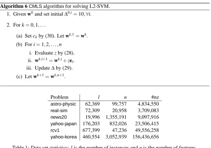
Algorithm 6CMLSalgorithm for solving L2-SVM. 1. Given w0and set initial∆0,i=10,∀i.
2. For k=0,1, . . .
(a) Set ck by (30). Let wk,1=wk. (b) For i=1,2, . . . ,n
i. Evaluate z by (28). ii. wk,i+1=wk,i+zei. iii. Update∆by (29).
(c) Let wk+1=wk,n+1.
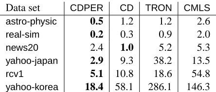
Problem l n #nz
astro-physic 62,369 99,757 4,834,550
real-sim 72,309 20,958 3,709,083
news20 19,996 1,355,191 9,097,916
yahoo-japan 176,203 832,026 23,506,415
rcv1 677,399 47,236 49,556,258
yahoo-korea 460,554 3,052,939 156,436,656
Table 1: Data set statistics: l is the number of instances and n is the number of features.
and set the initial w=0 and∆0,i=10,∀i. We find that the result is insensitive to these parameters. The detail ofCMLSalgorithm is listed in Algorithm 6.
Zhang and Oles (2001) prove that if ck =0,∀k, then the objective function of (3) is decreasing after each inner iteration. However, such a property may not imply that Algorithm 6 converges to the minimum. In addition,CMLSupdates w by (28), which is more conservative than Newton steps. In Section 5, we show thatCMLStakes more time and iterations than ours to obtain a solution.
5. Experiments and Analysis
In this section, we conduct two experiments to investigate the performance of our proposed coor-dinate descent algorithm. The first experiment compares our method with other L2-SVM solvers in terms of the speed to reduce function/gradient values. The second experiment evaluates various state of the art linear classifiers for L1-SVM, L2-SVM, and logistic regression. We also discuss the stopping condition of these methods.
5.1 Data Sets
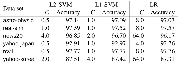
Data set CDPER CD TRON CMLS
astro-physic 0.5 1.2 1.2 2.6
real-sim 0.2 0.3 0.9 2.0
news20 2.4 1.0 5.2 5.3
yahoo-japan 2.9 9.3 38.2 13.5
rcv1 5.1 10.8 18.6 54.8
yahoo-korea 18.4 58.1 286.1 146.3
Table 2: The training time for an L2-SVM solver to reduce the objective value to within 1% of the optimal value. Time is in seconds. We use C=1. The approach with the shortest running time is boldfaced.
athttp://www.csie.ntu.edu.tw/˜cjlin/libsvmtools/datasets. A brief reminder for each data set can be found below.
• astro-physic: This set is a classification problem of scientific papers from Physics ArXiv.
• real-sim: This set includes some Usenet articles.
• news20: This is a collection of news documents, and was preprocessed by Keerthi and De-Coste (2005).
• yahoo-japan: We use binary term frequencies and normalize each instance to unit length.
• rcv1: This set (Lewis et al., 2004) is an archive of manually categorized newswire stories from Reuters Ltd. Each vector is a cosine normalization of a log transformed TF-IDF (term frequency, inverse document frequency) feature vector.
• yahoo-korea: Similar to yahoo-japan, we use binary term frequencies and normalize each instance to unit length.
To examine the testing accuracy, we use a stratified selection to split each set to 4/5 training and 1/5 testing.
5.2 Comparisons
We compare the following six implementations.TRON-LRis for logistic regression,Pegasosis for L1-SVM, and all others are for L2-SVM.
1. CD: the coordinate descent method described in Section 2. We chooseσin (12) as 0.01.
2. CDPER: the method modified fromCDby permuting sub-problems at each outer step. See the discussion in Section 3.2.
3. CMLS: a coordinate descent method for L2-SVM (Zhang and Oles, 2001, Algorithm 3). It is discussed in Section 4.3.
Data set L2-SVM L1-SVM LR
C Accuracy C Accuracy C Accuracy
astro-physic 0.5 97.14 1.0 97.09 8.0 97.03
real-sim 1.0 97.59 1.0 97.52 8.0 97.57
news20 4.0 96.85 2.0 96.70 64.0 96.17
yahoo-japan 0.5 92.91 1.0 92.97 4.0 92.76
rcv1 0.5 97.77 1.0 97.77 8.0 97.76
yahoo-korea 2.0 87.51 4.0 87.42 64.0 87.31
Table 3: The best parameter C and the corresponding testing accuracy of L1-SVM, L2-SVM and logistic regression (LR). We conduct five-fold cross validation to select C.
5. TRON-LR: the trust region Newton method for logistic regression introduced by Lin et al.. Similar toTRON, we use the implementation in the softwareLIBLINEARwith option-s 0.
6. Pegasos: the primal estimated sub-gradient solver for L1-SVM (Shalev-Shwartz et al., 2007). See the discussion in Section 4.1. The source code is available online at http://ttic. uchicago.edu/˜shai/code.
We do not include the bias term in all the solvers. All the above algorithms are implemented in C++ with double-precision floating-point numbers. Using single precision (e.g., Bottou, 2007) may reduce the computational time in some situations, but this setting may cause numerical inaccuracy. We conduct experiments on an Intel 2.66GHz processor with 8GB of main memory under Linux.
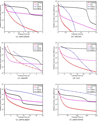
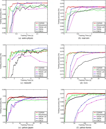
In our first experiment, we compare L2-SVM solvers (with C=1) in term of the speed to reduce function/gradient values. In Table 2, we check their CPU time of reducing the relative difference of the function value to the optimum,
f(wk)−f(w∗)
|f(w∗)| , (31)
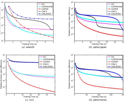
to within 0.01. We runTRONwith the stopping conditionk∇f(wk)k ≤0.01 to obtain the reference solutions. Since objective values are stable under such strict stopping conditions, these solutions are seen to be very close to the optima. Overall, our proposed algorithmsCDPERandCDperform well on all the data sets. For the large data sets (rcv1, yahoo-japan, yahoo-korea),CD is significantly better thanTRON andCMLS. With the permutation of sub-problems, CDPERis even better than CD. To show more detailed comparisons, Figure 1 presents time versus relative difference (31). As a reference, we draw a horizontal dotted line to indicate the relative difference 0.01. Consistent with the observation in Table 2,CDPERis more efficient and stable than others.
In addition, we are interested in how fast these methods decrease the norm of gradients. Figure 2 shows the result. Overall,CDPERconverges faster in the beginning, whileTRONis the best for final convergence.
0 0.5 1 1.5 2 2.5 3 3.5 4 10−6
10−4 10−2 100
Training Time (s)
Relative function value difference
CDPER CD TRON CMLS
(a)astro-physic
0 0.5 1 1.5 2 2.5
10−4 10−3 10−2 10−1 100 101
Training Time (s)
Relative function value difference
CDPER CD TRON CMLS
(b)real-sim
0 1 2 3 4 5 6
10−4 10−3 10−2 10−1 100 101
Training Time (s)
Relative function value difference
CDPER CD TRON CMLS
(c) news20
0 5 10 15 20 25 30
10−4 10−3 10−2 10−1 100 101
Training Time (s)
Relative function value difference
CDPER CD TRON CMLS
(d)rcv1
0 5 10 15 20 25 30
10−4 10−3 10−2 10−1 100 101
Training Time (s)
Relative function value difference
CDPER CD TRON CMLS
(e)yahoo-japan
0 50 100 150 200
10−4 10−3 10−2 10−1 100 101
Training Time (s)
Relative function value difference
CDPER CD TRON CMLS
(f)yahoo-korea
0 0.5 1 1.5 2 2.5 3 3.5 4 10−3
10−2 10−1 100 101 102
Training Time (s)
||Gradient||
CDPER CD TRON CMLS
(a)astro-physic
0 0.5 1 1.5 2 2.5
10−2 10−1 100 101 102 103
Training Time (s)
||Gradient||
CDPER CD TRON CMLS
(b)real-sim
0 1 2 3 4 5 6
100 101 102
Training Time (s)
||Gradient||
CDPER CD TRON CMLS
(c) news20
0 5 10 15 20 25 30
100 101 102 103 104
Training Time (s)
||Gradient||
CDPER CD TRON CMLS
(d)rcv1
0 5 10 15 20 25 30
101 102 103
Training Time (s)
||Gradient||
CDPER CD TRON CMLS
(e)yahoo-japan
0 50 100 150 200
101 102 103 104
Training Time (s)
||Gradient||
CDPER CD TRON CMLS
(f)yahoo-korea
0 0.5 1 1.5 2 0.965 0.966 0.967 0.968 0.969 0.97 0.971 0.972
Training Time (s)
Testing accuracy (%) CDPER PEGASOS TRON−LR TRON CMLS
(a)astro-physic
0 0.5 1 1.5
0.96 0.962 0.964 0.966 0.968 0.97 0.972 0.974 0.976 0.978 0.98
Training Time (s)
Testing accuracy (%) CDPER PEGASOS TRON−LR TRON CMLS
(b)real-sim
0 2 4 6 8 10
0.955 0.96 0.965 0.97
Training Time (s)
Testing accuracy (%) CDPER PEGASOS TRON−LR TRON CMLS
(c) news20
0 5 10 15 20 25 30
0.97 0.971 0.972 0.973 0.974 0.975 0.976 0.977 0.978 0.979 0.98
Training Time (s)
Testing accuracy (%) CDPER PEGASOS TRON−LR TRON CMLS
(d)rcv1
0 5 10 15 20 25 30
0.91 0.915 0.92 0.925 0.93 0.935
Training Time (s)
Testing accuracy (%) CDPER PEGASOS TRON−LR TRON CMLS
(e)yahoo-japan
0 50 100 150 200
0.84 0.845 0.85 0.855 0.86 0.865 0.87 0.875 0.88
Training Time (s)
Testing accuracy (%) CDPER PEGASOS TRON−LR TRON CMLS
(f)yahoo-korea
testing set. Table 3 presents the testing accuracy. Notice that some solvers scale the SVM formu-lation, so we adjust their regularization parameter C accordingly.2 With the best parameter setting, SVM (L1 and L2) and logistic regression give comparable generalization performances. In Figure 3, we present the testing accuracy along the training time. As an accurate solution of the SVM op-timization problem does not imply the best testing accuracy, some implementations achieve higher accuracy before reaching the minimal function value. Below we give some observations of the experiments.
We do not includeCDin Figure 3, becauseCDPERis better than it in almost all situations. One may ask if simply shuffling features once in the beginning can give similar performances toCDPER. Moreover, we can apply permutation schemes toCMLSas well. In Section 6.1, we give a detailed discussion on the issue of feature permutations.
Regarding the online setting of randomly selecting only one feature at each step (Algorithm 3), we find that results are similar to those ofCDPER.
From the experimental results, CDPERconverges faster than CMLS. Both are coordinate de-scent methods, and the cost per iteration is similar. However,CMLSsuffers from lengthy iterations because its modified Newton method takes a conservative step size. In Figure 3(d), the testing accu-racy even does not reach a reasonable value after 30 seconds. Conversely,CDPERusually uses full Newton steps, so it converges faster. For example,CDPERtakes the full Newton step in 99.997% inner iterations for solvingrcv1(we check up to 5.96 seconds).
Though Pegasosis efficient for several data sets, the testing accuracy is sometimes unstable (see Figure 3(c)). AsPegasosonly subsamples one training data to update wk, it is influenced more by noisy data. We also observe slow final convergence on the function value. This slow convergence may make the selection of stopping conditions (maximal number of iterations for Pegasos) more difficult.
Finally, compared toTRON andTRON-LR,CDPERis more efficient to yield good testing ac-curacy (See Table 2 and Figure 3); however, if we check the value||∇f(wk)||, Figure 2 shows that
TRON converges faster in the end. This result is consistent with what we discussed in Section 1 on distinguishing various optimization methods. We indicated that a Newton method (whereTRON is) has fast final convergence. Unfortunately, since the cost per TRON iteration is high, and the Newton direction is not effective in the beginning, TRONis less efficient in the early stage of the optimization procedure.
5.3 Stopping Conditions
In this section, we discuss stopping conditions of our algorithm and other existing methods. In solving a strictly convex optimization problem, the norm of gradients is often considered in the stopping condition. The reason is that
k∇f(w)k=0 ⇐⇒ w is the global minimum.
For example,TRON checks whether the norm of gradient is small enough for stopping. However, as our coordinate descent method updates one component of w at each inner iteration, we have only
D0i(0) =∇f(wk,i)
i,i=1, . . . ,n. Theorem 2 shows that wk,i→w∗, so we have
D0i(0) =∇f(wk,i)i→0,∀i.
0 1 2 3 4 5 6 10−4
10−3 10−2 10−1 100 101
Training Time (s)
Relative function value difference
CD CDPERONE CDPER CMLS CMLSPER
(a)news20
0 5 10 15 20 25 30
10−4 10−3 10−2 10−1 100 101
Training Time (s)
Relative function value difference
CD CDPERONE CDPER CMLS CMLSPER
(b)yahoo-japan
0 5 10 15 20 25 30
10−4 10−3 10−2 10−1 100 101
Training Time (s)
Relative function value difference
CD CDPERONE CDPER CMLS CMLSPER
(c)rcv1
0 50 100 150 200
10−4 10−3 10−2 10−1 100 101
Training Time (s)
Relative function value difference
CD CDPERONE CDPER CMLS CMLSPER
(d)yahoo-korea
Figure 4: Results of different orders of sub-problems at each outer iteration. We present time versus the relative difference of the objective value to the minimum. Time is in second.
Therefore, by storing Di(0),∀i, at the end of the kth iteration, one can check if ∑ni=1D0i(0)2 or maxi|D0i(0)|is small enough. ForPegasos, we mentioned in Section 4.1 that one may need a maxi-mal number of iterations as the stopping condition due to the lack of function/gradient information. Another possible condition is to check the validation accuracy. That is, the training procedure ter-minates after reaching a stable validation accuracy value.
6. Discussion and Conclusions
In this section, we discuss some related issues and give conclusions.
6.1 Order of Sub-problems at Each Outer Iteration
of sub-problems (CDPERandCD), with permutation only once before training (CDPERONE), and CMLSwith/without permuting sub-problems (CMLSandCMLSPER). Figure 4 shows the relative difference of the objective value to the minimum along time. Overall,CDPERconverges faster than CDPERONEandCD, butCMLSPERdoes not improve overCMLSmuch.
With the permutation of features at each iteration, the cost perCDPERiteration is slightly higher thanCD, butCDPERrequires much fewer iterations to achieve a similar accuracy value. This result seems to indicate that if the sub-problem order is fixed, the update of variables becomes slower. However, asCD sequentially accesses features, it has better data locality in the computer memory hierarchy. An example isnews20in Figure 4(a). As the number of features is much larger than the number of instances, two adjacent sub-problems ofCDPERmay access two very far away features. Then the cost per CD iteration is only 1/5 ofCDPER, soCD is better in the beginning. CDPER catches up in the end due to its faster convergence.
ForCMLSandCMLSPER, the latter is only faster in the final stage (see the right end of Figures 4(b) and 4(d)). Since the function reduction ofCMLS(orCMLSPER) is slow, the advantage of doing permutations appears after long training time.
The main difference betweenCDPERONEandCDPERis that the former only permutes features once in the beginning. Figure 4 clearly shows thatCDPERis better thanCDPERONE, so permuting features only once is not enough. If we compareCDandCDPERONE, there is no definitive winner. This result seems to indicate that feature ordering affects the performance of the coordinate descent method. By using various feature orders,CDPERavoids taking a bad one throughout all iterations.
6.2 Coordinate Descents for Logistic Regression
We can apply the proposed coordinate descent method to solve logistic regression, which is twice differentiable. An earlier study of using coordinate decent methods for logistic regression/maximum entropy is by Miroslav et al. (2004). We compare an implementation withTRON-LR. Surprisingly, our method is not better in most cases. Experiments show that for training rcv1, our coordinate descent method takes 93.1 seconds to reduce the objective value to within 1% of the optimal value, while TRON-LR takes 27.9 seconds. Only foryahoo-japanandyahoo-korea, where TRON-LRis slow (see Figure 3), the coordinate descent method is competitive. This result is contrast to earlier experiments for L2-SVM, where the coordinate descent method more quickly obtains a useful model thanTRON. We give some explanations below.
With the logistic loss, the objective function is (4). The single-variable function Di(z)is non-linear, so we use Algorithm 2 to obtain an approximate minimum. To use the Newton direction, similar to D0i(z)and D00i(z)in (9) and (10), we need
D0i(0) =∇if(w) =wi+C
∑
j:xji6=0−yjxjie−yjw
Tx j
1+e−yjwTxj ,
D00i(0) =∇2iif(w) =1+C
∑
j:xji6=0x2
jie−yjw
Tx j
(1+e−yjwTxj)2,
where we abbreviate wk,i to w, and use yj =±1. Then|{j|xji6=0}|exponential operations are conducted. If we assume thatλ=1 satisfies the sufficient decrease condition (12), then the cost per outer iteration is
This complexity is the same as (19) for L2-SVM. However, since each exponential operation is ex-pensive (equivalent to tens of multiplications/divisions), in practice (32) is much more time consum-ing. ForTRON-LR, a trust region Newton method, it calculates∇f(w)and∇2f(w)at the beginning of each iteration. Hence l exponential operations are needed for exp(−yjwTxj),j=1, . . . ,l. From (27), the cost per iteration is
O(#nz)×(# conjugate gradient iterations) + (l exponential operations). (33)
Since l#nz, exponential operations are not significant in (33). Therefore, the cost per iteration of applying trust region Newton methods to L2-SVM and logistic regression does not differ much. In contrast, (32) shows that coordinate descent methods are less suitable for logistic regression than L2-SVM. However, we may avoid expensive exponential operations if all the elements of xjare either 0 or the same constant. By storing exp(−yjwTxj),j=1, . . . ,l, one updates exp(−yj(wk,i)Txj)by multiplying it by exp(−zyjxji). Using yj=±1, exp(−zyjxji) = (exp(−zxji))yj. As xji is zero or a constant for all j, the number of exponential operations per inner iteration is reduced to one. In addition, applying fast approximations of exponential operations such as Schraudolph (1999) may speed up the coordinate descent method for logistic regression.
6.3 Conclusions
In summary, we propose and analyze a coordinate descent method for large-scale linear L2-SVM. The new method possesses sound optimization properties. The method is suitable for data with an easy access of any feature. Experiments indicate that our method is more stable and efficient than most existing algorithms. We plan to extend our work to other challenging problems such as training large data which can not fit into memory.
Acknowledgments
This work was supported in part by the National Science Council of Taiwan grant 95-2221-E-002-205-MY3. The authors thank Associate Editor and reviewers for helpful comments.
Appendix A. Proofs
In this section, we prove theorems appeared in the paper. First, we discuss some properties of our objective function f(w). Consider the following piecewise quadratic strongly convex function:
g(s) =1
2s
Ts+Ck(As−h)
+k2, (34)
where(·)+ is the operator that replaces negative components of a vector with zeros. Mangasarian
(2002) proves the following inequalities for all s,v∈Rn:
(∇g(s)−∇g(v))T(s−v) ≥ ks−vk2, (35)
|g(v)−g(s)−∇g(s)T(v−s)| ≤ K
2kv−sk
2, (36)
where
Our objective function f(w) is a special case of (34) with A=Y X (X is defined in Eq. 20) and
h=−1, where Y is a diagonal matrix with Yj j=yj, j=1, . . . ,l and 1 is the vector of all ones. With yi=±1, f(w)satisfies (35) and (36) with
K=1+2CkXk22. (37)
To derive properties of the subproblem Di(z)(defined in Eq. 8), we set
A=−
y1x1i
.. .
ylxli
and h=
y1wTx1−y1wix1i−1
.. .
ylwTxl−ylwixli−1
,
where we abbreviate wk,ito w. Since
Di(z) =
1 2w
Tw
−12w2i +
1
2(z+wi)
2+
k(A(z+wi)−h)+k2
,
the first and second terms of the above form are constants. Hence, Di(z)satisfies (35) and (36) with
K=1+2C
l
∑
j=1
x2ji.
We use Hi to denote Di(z)’s corresponding K. This definition of Hiis the same as the one in (14). We then derive several lemmas.
Lemma 5 For any i∈ {1, . . . ,n}, and any z∈R,
D0i(0)z+1
2Hiz
2
≥Di(z)−Di(0)≥D0i(0)z+ 1 2z
2. (38)
Proof There are two inequalities in (38). The first inequality directly comes from (36) using Di(z) as g(s)and Hias K. To derive the second inequality, if z<0, using Di(z)as g(s)in (35) yields
D0i(z)≤D0i(0) +z.
Then,
Di(z)−Di(0) =−
Z 0
t=z
D0i(t)dt≥D0i(0)z+1
2z
2.
The situation for z≥0 is similar.
Lemma 6 There exists a unique optimum solution for (3).
Proof From Weierstrass’ Theorem, any continuous function on a compact set attains its minimum.
We consider the level set A={w| f(w)≤ f(0)}. If A is not bounded, there is a sub-sequence
{wk} ⊂A such thatkwkk →∞. Then
f(wk)≥1
2kw
kk2→∞.
A.1 Proof of Theorem 1
Proof By Lemma 5, we let z=λd and have
Di(λd)−Di(0) +σλ2d2
≤ D0i(0)λd+1
2Hiλ
2d2+σλ2d2 = −λD0i(0)2
D00i(0) +
1 2Hiλ
2D0i(0)2
D00i(0)2+σλ
2D0i(0)2
D00i(0)2
= λD0i(0)2
D00i(0)
λ(Hi/2+σ
D00i(0) )−1
. (39)
If we choose ¯λ= D00i(0)
Hi/2+σ, then for λ≤
¯
λ, (39) is non-positive. Therefore, (12) is satisfied for all 0≤λ≤λ¯.
A.2 Proof of Theorem 2 (convergence of Algorithm 1)
Proof By settingπk(i) =i, this theorem is a special case of Theorem 3.
A.3 Proof of Theorem 3 (Convergence of Generalized Algorithm 1) Proof To begin, we define 1-norm and 2-norm of a vector w∈Rn:
kwk1=
n
∑
i=1
|wi|, kwk2= s
n
∑
i=1
w2i.
The following inequality is useful:
kwk2≤ kwk1≤√nkwk2, ∀w∈Rn. (40)
By Theorem 1, anyλ∈[βλ¯,λ¯]satisfies the sufficient decrease condition (12), whereβ∈(0,1)
and ¯λis defined in (14). Since Algorithm 2 selectsλby trying{1,β,β2, . . .}, the valueλselected
by Algorithm 2 satisfies
λ≥βλ¯ = β
Hi/2+σ
D00π
k(i)(0).
This and (13) suggest that the step size z=λd in Algorithm 2 satisfies
|z|=λ
−D0π
k(i)(0)
D00π
k(i)(0)
≥
β
Hi/2+σ|
D0π
k(i)(0)|. (41)
Assume
H=max(H1, . . . ,Hn)andγ= β
We use w and f(w)to rewrite (41):
|wkπ,i+1
k(i) −w
k,i
πk(i)| ≥γ|∇f(w
k,i)
πk(i)|, (43)
where we use the fact
D0π
k(i)(0) =∇f(w
k,i) πk(i).
Taking the summation of (43) from i=1 to n, we have
kwk+1−wkk1≥γ
n
∑
i=1
|∇f(wk,i)πk(i)|
≥γ
n
∑
i=1
(|∇f(wk,1)πk(i)| − |∇f(wk,i)πk(i)−∇f(w
k,1)
πk(i)|)
=γ k∇f(wk,1)k1−
n
∑
i=1
|∇f(wk,i)πk(i)−∇f(wk,1)πk(i)|
!
.
(44)
By the definition of f(w)in (3),
∇f(w) =w−2C
l
∑
j=1
yjxjmax(1−yjwTxj,0).
With yj=±1,
n
∑
i=1
|∇f(wk,i)πk(i)−∇f(wk,1)πk(i)|
≤
n
∑
i=1 |wkπ,i
k(i)−w
k,1
πk(i)|+2C
l
∑
j=1
|xjπk(i)| |(w
k,i)Tx
j−(wk,1)Txj|
!
≤
n
∑
i=1
|wkπ+1
k(i)−w
k
πk(i)|+2C
l
∑
j=1 |xjπk(i)|
n
∑
q=1
|xjq| |wkq,i−wkq,1|
!
=kwk+1−wkk1+2C
n
∑
i=1
l
∑
j=1
n
∑
q=1
|xjπk(i)| |xjq| |wkq,i−wkq,1|
≤kwk+1−wkk1+2C n
∑
q=1
|wkq+1−wkq|
∑
i,j:xjπk(i)6=0P2
=(1+2CP2(#nz))kwk+1−wkk1,
(45)
where P is defined in (6). From (44) and (45), we have
kwk+1−wkk1≥ γ
1+γ+2γCP2(#nz)k∇f(w
k,1)k1.
With (40),
kwk+1−wkk2≥
1
√
nkw
k+1 −wkk1
≥√ γ
n(1+γ+2γCP2(#nz))k∇f(w
k)
k1≥√ γ
n(1+γ+2γCP2(#nz))k∇f(w
k)
k2.
From Lemma 6, there is a unique global optimum w∗for (3). The optimality condition shows that
∇f(w∗) =0. (47)
From (35) and (47),
kwk−w∗k2≤ k∇f(wk)−∇f(w∗)k2=k∇f(wk)k2. (48)
With (46),
kwk+1−wkk2≥τkwk−w∗k2, whereτ=
γ
√
n(1+γ+2γCP2(#nz)). (49)
From (12) and (49),
f(wk)−f(wk+1) =
n
∑
i=1
(f(wk,i)−f(wk,i+1))
≥
n
∑
i=1
σ(wkπ,i+1
k(i) −w
k,i πk(i))
2=σ
kwk+1−wkk22≥στ2kwk−w∗k22.
By (36) and (47),
f(wk)−f(w∗)≤K
2kw
k−w∗k2
2, (50)
where K is defined in (37). Therefore, we have
f(wk)−f(wk+1)≥2στ
2
K (f(w
k)
−f(w∗)).
This is equivalent to
(f(wk)−f(w∗)) + (f(w∗)−f(wk+1))≥2στ 2
K (f(w
k)
−f(w∗)).
Finally, we have
f(wk+1)−f(w∗)≤(1−2στ
2
K )(f(w
k)
−f(w∗)). (51)
Withτ≤1 from (49), K≥1 from (37) andσ<1/2, we have 2στ2/K<1. Hence, (51) ensures that f(wk)approaches f(w∗).
From (51),{f(wk)}converges to f(w∗). We can then prove that{wk}globally converges to w∗. If this result does not hold, there is a sub-sequence{wk}Mconverging to a point ¯w6=w∗. However, Lemma 6 shows that f(w)¯ > f(w∗), so limk∈M f(wk)> f(w∗), a contradiction.
Let µ=2στ2/K, (51) implies
f(wk)−f(w∗)≤(1−µ)k(f(w0)−f(w∗)), ∀k.
To achieve anε-accurate solution, we need the right-hand side to be smaller thanε. Thus,
k≥log(f(w
0)−f(w∗)) +log(1/ε)
From the inequality
log(1−x)≤ −x if x<1,
we have
k≥log(f(w
0)−f(w∗)) +log(1/ε)
µ . (52)
In following we discuss the order of µ−1= K
2στ2. From (37),
K=2CkXk2
2+1≤2CkXk2F+1≤2CP2(#nz) +1, (53) wherek · kF is the Frobenious norm. From (49),
τ−1=√n
1
γ+2CP2(#nz) +1
.
Sinceγ=σ+βH/2, from (14) and (42) we have
γ−1=O(lCP2+1)
≤O(CP2(#nz) +1). (54) As #nz is usually large, we omit the constant term O(1) in the following discussion. Thenτ−1=
O(√nCP2(#nz)). Thus,
µ−1= K
2στ2 =O(nC
3P6(#nz)3). (55)
From (52) and (55), Algorithm 1 obtains anε-accurate solution in
O nC3P6(#nz)3log(1/ε)
iterations.
A.4 Proof of Theorem 4 (Linear Convergence of the Online Setting)
Proof To begin, we denote the expectation value of a function g of a random variable y to be
Ey(g(y)) =
∑
y
P(y)g(y).
Then for any vector s∈Rnand a random variable I where
P(I=i) =1
n,∀i∈ {1, . . . ,n},
we have
EI(s2I) =
n
∑
i=1
s2i
n =
1
nksk
2
2. (56)
At each iteration k (k=0,1, . . .) of Algorithm 3, we randomly choose one index ik and update wk to wk+1. The expected function value after iteration k can be represented as
Ei0,...,ik−1,ik(f(w