Observer-Based Robust Adaptive Fuzzy Control for
Uncertain Underactuated Systems with Time Delay and
Dead-Zone Input
Chiang-Cheng Chiang*, Li-Chung Chang
Department of Electrical Engineering, Tatung University, Taipei, Taiwan, Republic of China
Abstract This paper investigates the observer-based robust adaptive fuzzy control problem for a class of uncertain
underactuated systems with time delay and dead-zone input. Within this method, the state observer is developed for estimating the unmeasured states in the underactuated system. The fuzzy logic systems are used to approximate the unknown nonlinear functions, and some adaptive laws are introduced to estimate unknown parameters. The dead-zone input which is one of the significant input constraints often exists in many practical industrial control systems. By employing a Lyapunov-Krasovskii functional, it is verified that the proposed controller ensures that all the signals in the closed-loop system are bounded. Simulation results are illustrated to demonstrate the regulation performance of the system output and state estimation by the proposed control method.Keywords Underactuated system, Lyapunov-Krasovskii functional, Dead-zone input, Fuzzy logic systems, State
observer, Time delay1. Introduction
In the past decades, the control problem of underactuated systems has received a lot of attention. The underactuated system is a mechanical system with fewer control actuators than degrees of freedom and can be found in many applications, such as boom cranes [1], axisymmetric spacecrafts [2], pole and hoop systems [3], surface vessels [4], and so on. The underactuated systems have some advantages like decreasing the number of actuators, reducing the cost, and lightening the system.
The dead-zone input nonlinearity is a nonsmooth function that features certain insensitivity for small control inputs which is often encountered in a variety of practical systems, such as the valve system [5] and the gripper rotating system [6]. The adaptive fuzzy controller is proposed to deal with nonlinear systems with unknown dead zones [7]. In [8], the adaptive tracking control problems are considered for a class of nonlinear systems with a fuzzy dead-zone input.
A category of switched uncertain nonlinear systems were studied through using adaptive fuzzy output-feedback
* Corresponding author:
[email protected] (Chiang-Cheng Chiang) Published online at http://journal.sapub.org/control
Copyright©2019The Author(s).PublishedbyScientific&AcademicPublishing This work is licensed under the Creative Commons Attribution International License (CC BY). http://creativecommons.org/licenses/by/4.0/
control in [9]. In [10], a robust adaptive fuzzy tracking controller was designed for pure-feedback stochastic nonlinear systems with input constraints. On the other hand, Zhou et al. [11] deal with the problem of adaptive fuzzy control for nonstrict-feedback systems with input saturation and output constraint. In this paper, fuzzy logic systems are introduced to describe the input/output behavior of the controlled system. Based on fuzzy logic systems, we design the adaptive fuzzy controllers with several appropriate adaptive laws.
In many practical systems, system states are not available for measurement. Based on state variable filters, an observer is presented for solving the problem of the unavailable states of the system. Recently, for a class of uncertain nonlinear systems with nonsymmetric input saturation, the problem of observer-based adaptive NN control was considered in [12]. In [13], a fuzzy state observer was proposed to estimate the unmeasured states.
It is well known that the time-delay systems have received considerable attention [14], [15], and the existence of time delay often leads to the system instability and poor performance. Based on Lyapunov-Krasovskii functional, the presented robust adaptive fuzzy control method can ensure the robust stability of the whole closed-loop nonlinear system with time delay.
unknown nonlinear functions, and a fuzzy state observer is constructed to estimate the unmeasurable system states. Some appropriate adaptive laws are used to estimate the upper bounds of the unknown uncertainties. Finally, with the help of Lyapunov stability theorem, the proposed controller can guarantee the stability of the system.
The rest of this paper is organized as follows. The description of the system and the concept of fuzzy logic systems are presented together in Section II. The observer-based robust adaptive fuzzy controller is designed in Section III for uncertain underactuated system with time delay and dead-zone input. In Section IV, the numerical example and the practical example are provided to validate the effectiveness of the proposed observer-based robust adaptive fuzzy control approach. Section V contains the conclusion.
2. Problem Statement and Preliminaries
2.1. System DescriptionConsider a class of single-input multi-output uncertain underactuated nonlinear systems with time delay and dead- zone input expressed as follows:
11 12
1 1
21 2 12
22
2
11 21
2
1 2
2
1 2
( )) ( ( )) , )
( )) ( ( )) , )
( (
( (
( ( )) ( ( )) ( , ) (t) [ , ,..., ]
n n n
T
n n
n
x t D u t t
x t D u t t
x t
x x
f
x x
f
x
D u t t
x x
x f
x τ
τ
τ
δ
δ
δ
= − +
= − +
= −
=
+ =
+
=
+
+
=
x x
x x
x x
y
(1)
where x=[x11,x12,...,xn1,xn2] T ∈ R2n×1 is the system state vector which is assumed to be unavailable for measurement, u(t)∈Rnand y( )t ∈Rn×1 are the input and output of the system, respectively. τis the value of time delay f1( (x t−τ)) , f2( (xt−τ)) ,…, fn(x(t−τ)) are unknown real continuous nonlinear functions, and δ1( , )xt ,
2( , )t
δ x ,…,δn(x, )t are the unknown bounded disturbances. ( ( ))
D u t :R→R is the nonlinear input function containing a dead zone.
Assumption 1: The time delay τ is a fixed and known positive constant.
System (1) can be rewritten as
[ ( (t τ)) D u( (t)) + ( ,t ])
= + +
=
−
x Ax B f E δ x
y Cx x
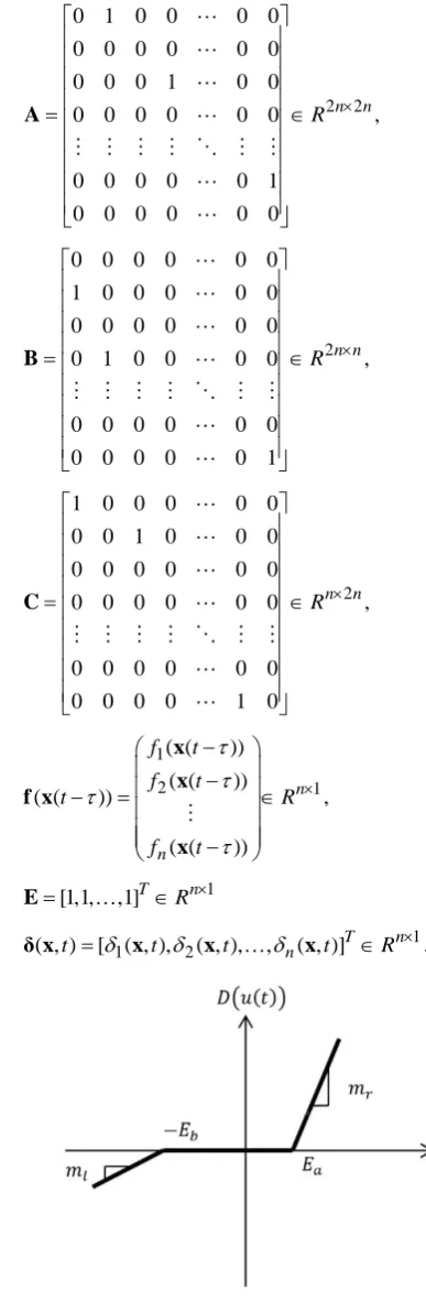
(2) where
2 2
0 1 0 0 0 0
0 0 0 0 0 0
0 0 0 1 0 0
,
0 0 0 0 0 0
0 0 0 0 0 1
0 0 0 0 0 0
n n
R ×
= ∈
A
2
0 0 0 0 0 0
1 0 0 0 0 0
0 0 0 0 0 0
,
0 1 0 0 0 0
0 0 0 0 0 0
0 0 0 0 0 1
n n
R ×
= ∈
B
2
1 0 0 0 0 0
0 0 1 0 0 0
0 0 0 0 0 0
,
0 0 0 0 0 0
0 0 0 0 0 0
0 0 0 0 1 0
n n R ×
= ∈
C
1
2 1
( ( )) ( ( )) ( ( ))
( ( ))
n
n
f t
f t
t R
f t
τ τ τ
τ
×
−
−
− = ∈
−
x x f x
x
,
1
[1,1, ,1]T Rn×
= ∈
E
1
1 2
( , )t =[δ ( , ,t)δ ( ,t), ,δn( , ]t)T∈Rn×
δ x x x x .
Figure 1. Dead-zone model
( ( ) ) for ( ) ( ( )) 0 for ( )
( ( ) ) for ( )
r a a
b a
l b b
m u t E u t E
D u t E u t E
m u t E u t E
− ≥
= − ≤ ≤
+ ≤ −
(3)
where Ea,Eb,mr and ml are parameters and slopes of the dead zone, respectively.
To investigate the key features of the dead zone in the control problems, the following common assumptions are given.
Assumption 2: The dead-zone output D u t( ( )) is not available to obtain.
Assumption 3: The coefficients Ea,Eb,mr and m l are unknown.
Assumption 4: There exist known constants mmin,mmax,
min a
E ,Eamax,Ebmin and Ebmax such that the unknown dead-zone parameters mr,ml,Ea and Eb are bounded, i.e. 0<m mr, l∈[mmin,mmax], 0<Ea∈[Eamin, ]Eamax ,
0<Eb∈[Ebmin, ]Ebmax .
Based on the above assumptions, the expression (3) can be rewritten as
( ( )) ( ) ( ( ))
D u t =mu t +d u t (4) where d u t( ( )) can be calculated from (3) and (4) as
, for ( )
( ( )) ( ), for E ( ) , for ( )
r a a
b a
l b b
m E u t E
d u t mu t u t E
m E u t E
− ≥
= − − ≤ ≤
≤ −
(5)
From Assumption 4, it can be concluded that d u t( ( )) is bounded, and satisfies:
( ( ))
d u t ≤ρ (6) where ρ is the upper bound, which can be chosen as
{
m Er a, m El b}
ρ = (7)
Assumption 5: 0< δ x
( )
,t ≤ < ∞h , where h is an unknown constant.Control objective: The control objective is to design a robust adaptive fuzzy controller ( )u t to ensure that all the closed-loop signals are bounded.
2.2. Description of Fuzzy Logic Systems
The fuzzy logic system performs a mapping from n
U ⊂R toV ⊂R. Let U=U1× × Un where Ui⊂R, 1, 2, ,
i= n. The fuzzy rule base consists of a collection of fuzzy IF-THEN rules:
( )
1 1 2 2
: IF is , and is , and and, is
THEN is , for 1, 2, , .
l l l l
n n l
R x F x F x F
y G l= M
(8)
in which x=
[
x x1, 2,,xn]
T∈U and y∈ ⊂V R are theinput and output of the fuzzy logic system, Fil and Gl are fuzzy sets in Ui and V , respectively. The fuzzifier maps a crisp point x=
[
x x1, 2,,xn]
Tinto a fuzzy set in U.The fuzzy systems with center-average defuzzifier, product inference and singleton fuzzifier are of the following form:
( )
T
y=θ ξ x (9) where θT = θ1,,θB with each variable θl as the point at which the fuzzy membership function of
l
G achieves the maximum value and
1
( )= ξ ( ),...,ξM( )T
ξ x x x with each variable ξl( )x as the fuzzy basis function defined as
1
1 1
( ) ( )
( ) n
l i i F
l i
M n
l i i Fi l
x
x µ ξ
µ
=
= =
=
∏
∑ ∏
x (10)
where l( )i
Fi x
µ is the membership function of the fuzzy set.
3. Controller Design and Stability
Analysis
3.1. Observer Design
First, the following fuzzy logic systems can be constructed, over a compact set Γ, the unknown nonlinear functions ( )f x can be approximated as
ˆ( ( - ) |ˆ ) ˆT ( ) f f
t τ = t−τ
f x θ θ ξ(x ) (11) where ξ x( ( - ))t τ is the fuzzy basis vector, θˆf is the corresponding adjustableparameter vector of the fuzzy logic system.
Because the system states are assumed to be unmeasurable in this paper, the fuzzy logic systems (11) cannot be directly used for the unknown nonlinear system. Therefore, an observer is designed to estimate the unmeasurable system states. Let us define that ˆx is the estimate of x at first. Then, the following fuzzy logic systems can be obtained as
ˆf x( (ˆ t−τ) |θˆf)=θ ξ xˆTf ( (ˆ t−τ)) (12) The observer for system (2.2) is established as follows:
ˆ ˆ
ˆ ˆ ( (ˆ ) | ) ( ( )) ( ˆ)
ˆ ˆ
f
t τ D u t
= + − + + + −
=
x Ax B f x θ E ν L y y
y Cx
11 12
21
2 22
1 2
0 0 0 0 0
0 0 0 0 0
0 0 0 0 0
0 0 0 0 0 ,
0 0 0 0 0
0 0 0 0 0
n n
n n
l l
l
l R
l l
×
= ∈
L
1 2
1 1
n
n n
v v
R v
v
×
−
= ∈
v
L is the observer gain matrix to guarantee the characteristic polynomial of A - LC to be Hurwitz. The estimation error vector is defined as x=x - xˆ and y=y - yˆ, then according to (2) and (13), one has
ˆ ˆ ˆ
( ( (t τ)) ( (t τ) | f) ( , )t
= + − − − + −
=
x A - LC)x B f x f x θ δ x ν
y Cx
(14)
It is assumed that x, ˆx, and ˆθf belong to compact sets Ωx,Ωˆx, and Ωˆ
f
θ respectively, which is defined as
{
2 1}
Ωx = x∈R n× : x ≤Nx< ∞ (15)
{
2 1}
ˆ ˆ ˆ ˆ
Ωx = x∈R n× : x ≤Nx< ∞ (16)
{
}
ˆ ˆ ˆ
Ω f M n: f f
f R N
×
= ∈ ≤ < ∞
θ θ θ
(17)
where Nx,Nˆx, and Nf are the designed parameters, and M is the number of fuzzy inference rules. Let us define the optimal parameter vector θ *f as follows:
*
ˆ ˆ
ˆ ˆ ˆ arg min sup ( ( - )) ( ( - ) | )
f f
f f
t τ t τ
∈Ω ∈Γ
=
θ θ x
θ f x -f x θ (18)
where θ*f is bounded in the suitable closed set Ωˆ
f θ . The parameter estimation errors can be defined as
* ˆ
f = f − f
θ θ θ (19) and
*
ˆ ˆ
( ( - ))t τ ( (t τ) | f)
= − −
w f x f x θ (20) are the minimum approximation errors, which correspond to approximation errors obtained when optimal parameters are used.
According to (19) and (20), (14) can be written as
ˆ
( Tf ( (t τ)) ( , )t
= + − + + − =
x A - LC)x B θ ξ x w δ x ν
y Cx
(21)
The output error dynamic of (21) can be expressed as follows:
ˆ
( ) Tf ( ( )) ( , )
y=Hs θ ξ x t−τ + +w δ xt −ν (22) where H( )s =C( I - (A - LC)) Bs -1
and s denotes the complex Laplace transform variable.As previously discussed in this chapter, not all elements of x could be obtained, because not all the system states are available for measurement. Consequently, one could not obtain all elements of x. The state variable filters [17] will be introduced to cope with this problem. The stable filter
(s) u
G is chosen as follows:
0
1 ( )
u
G s
s g
=
+ (23)
for g0>0
( )s =diag G s G s[ u( ), u( ),...,G su( )]∈Rn n×
G (24)
Introducing (24) into (22), the steady-state equation can be written as
{ }
1
ˆ
( ) ( )s s − = ( )[s Tf ( (t−τ))+ + ( , )t − ]
G H y G θ ξ x w δ x ν (25)
Define a set of state variable filters Ti(s)=G( ) , s si
0,1
i= , thus,
0 0
0
1 ( )s ( )s s
s g
= = +
T G (26)
1
1 0
0
( )s ( )s s s ( )s s
s g
= = =
+
T G T (27)
The corresponding filtered signals are defined as follows:
{ }
{ }
1 0 1
2 1 1
, 1, 2,...,
f i i
f i i
x T x
i n
x T x
=
=
=
(28)
0( ){ } f = s
w T w (29)
0( ){ } f = s
ξ T ξ (30)
0( ){ } f = s
v T v (31)
0( ){ ( , )}
f = s t
δ T δ x (32) Eq. (21) can be rewritten as follows:
(
)
Tf ( (ˆ )) ( ,t)f f f f f f
f f
t τ
= − + − + + −
=
x A LC x B θ ξ x w δ x v y Cx
(33)
where
2 1
11 12 n1 2
[ , ,..., , ]T n
f = xf xf xf xfn ∈R ×
x
11 12
21
2 2 22
1 2
1 0 0 0 0
0 0 0 0 0
0 0 1 0 0
0 0 0 0 0
0 0 0 0 1
0 0 0 0 0
n n
n n l
l
l
l R
l l
×
−
−
−
−
− = ∈
−
−
A LC
It is assumed that there exists an unknown constant
1 0
w > , such that
1
f ≤w
w (34) Let us define that
1 1 ˆ1
w =w −w (35) and
ˆ
h= −h h (36) where wˆ1 and ˆh are the estimates of w1 and h , respectively.
Based on Lyapunov stable theorem, the robust compensation term νf and the parameter update laws can be obtained as follows:
1 ˆ
ˆ
T T
f f
f T T
f f
w h
=B Px +B Px
v
x PB x PB
(37)
ˆ ( ( - ))ˆ T f =γf f t τ f
θ ξ x x PB (38)
1 1
ˆ w Tf
w =γ x PB (39)
ˆ T
h f
h=γ x PB (40) where γf ,
1 w
γ , and γh are positive constants
Remark 1: Without loss of generality, the adaptive laws used in this paper are assumed that the parameter vectors are within the constraint sets or on the boundaries of the constraint sets but moving toward the inside of the constraint sets. If the parameter vectors are on the boundaries of the constraint sets but moving toward the outside of the constraint sets, we must use the projection algorithm to modify the adaptive laws such that the parameter vectors will remain inside of the constraint sets. Readers can refer to reference [16]. The proposed adaptive law (38) can be modified as the following form:
{
}
T , T ˆ( ( )) , if ( )
or (
ˆ ( (ˆ )) 0)
ˆ
( ( )) , if (
ˆ
and ( ( )) 0)
f
f f f f
f f
T f
f f f
T
f k
f f f f
T f f f t N N t
P t N
t
γ τ
τ γ τ
τ
− <
= = ⋅ − ≤ − =
⋅ − >
T
ξ x x PB θ
θ
θ x PB θ ξ x
ξ x x PB θ
x PB θ ξ x
(41)
where P
{
γfξ xf( (ˆ t−τ))x PBTf}
is defined as{
}
T 2 ˆ ( ( )) ˆ ˆ ˆ ˆ ( ( )) ( ( )) ˆ Tf f f
f f
T T
f f f f f f
f P t t t γ τ γ τ γ τ − = − − −
ξ x x PB
θ θ
ξ x x PB x PB ξ x
θ
(42)
The main result of the proposed robust adaptive fuzzy observer method is summarized on the following theorem.
Theorem 1: Consider the single-input multi-output uncertain underactuated system with time delay and dead-zone input (1). The robust adaptive fuzzy observer is defined by (13) with adaptation laws given by (37)-(40). For the given positive definite matrix Q, if there exists a symmetric positive definite matrix P such that the following Lyapunov equation
(
A LC−)
T P+P(
A−LC)
= −Q (43) is satisfied, then all the closed-loop signals are bounded, and the estimation errors converge to a neighborhood of zero.Proof: Consider the Lyapunov function candidate
(
)
2 21 1
1 1 1 1
2
T T
f f f f
f w h
V tr w h
γ γ γ
= + + + x Px θ θ
(44)
By the time derivate of V1 and the facts θf = −θˆf ,
1 ˆ1
w = −w ,h= −hˆ one has
(
)
( )
(
)
{
}
(
)
{
}
( )
1 1 1
1
1
1 1 ˆ 1 1 ˆ
ˆ 2 1 2 ˆ ( ( )) 1 2 ˆ ( ( ))
1 ˆ 1
T T T
f f f f f f
f w h
f
T T
f f f f f f
T
f f
T
f f f f f
T f f
f w
V tr w w hh
t t tr γ γ γ τ τ γ γ = + − − − = − + − + + − + − + − + + − − −
x Px x Px θ θ
A LC x
B θ ξ x w δ v Px
x P A LC x
B θ ξ x w δ v
θ θ
(
)
(
)
( )
1 1 1 1 1 1 ˆ ˆ 1 2 ˆ ( ( ))1 ˆ 1 1 ˆ
ˆ ˆ ( ( )) 1 h T T f f T T
f f f f f f
T f f
f w h
T T T T
f f f f f f f
T f f
f
w w hh
t
tr w w hh
t tr γ τ γ γ γ τ γ − = − + − + − + + − − − − + − + + − −
x A LC P P A LC x x PB θ ξ x w δ v
θ θ
x PBθ ξ x x PBw x PBδ
x PBv
( )
(
)
(
)
( )
1 1 1 1 1 11 1 ˆ
ˆ ˆ 1 2 ˆ ( ( ))
1 ˆ 1 1 ˆ
ˆ T f f w h T T f f
T T T T
f f f f f f f
T T
f f f f
f w h
w w hh
t
tr w w hh
γ γ τ γ γ γ − − ≤ − + − + − + + − − − − θ θ
x A LC P P A LC x
x PBθ ξ x x PB w x PB δ
x PBv θ θ
(45)
(
)
(
)
( )
1 1 1 1 1 1 2 ˆ + ( ( ))1 ˆ 1 1 ˆ
ˆ
T T
f f
T T T T
f f f f f
T T
f f f f
f w h
V
t w h
tr w w hh
τ γ γ γ ≤ − + − − + + − − − −
x A LC P P A LC x x PBθ ξ x x PB x PB
x PBv θ θ
(
)
(
)
(
)
( )
( )
1 1 1 1 1 1 1 2 ˆ ˆ ˆ + ( ( ))1 ˆ 1 1 ˆ
ˆ
T T
f f
T T T T
f f f f f
T T
f f f f
f w h
V
t w w h h
tr w w hh
τ γ γ γ = − + − − + + + + − − − −
x A LC P P A LC x
x PBθ ξ x x PB x PB x PBv θ θ
(46)
Substituting (38)-(40) into (46), one obtains
(
)
(
)
(
)
( )
(
)
(
)
(
)
(
)
1 1 1 1 1 1 1 2 ˆ ˆ ˆ + ( ( )) 1 ˆ( ) 1 1 1 2 T T f fT T T T
f f f f f
T T T
f f f f f f
f
T T
w f h f
w h
T T
f f
V
t w w h h
tr t w h τ γ τ γ γ γ γ γ ≤ − + − − + + + + − − − − − ≤ − + −
x A LC P P A LC x
x PBθ ξ x x PB x PB
x PBv θ ξ x x PB
x PB x PB
x A LC P P A LC x
1 ˆ ˆ
+ x PBTf w + x PBTf h−x PBvTf f
(47)
Considering the robust compensation term vf (37), the above equation can be rewritten as
(
)
(
)
1 1 2 T T f fV ≤ x A LC− P+P A LC− x (48) According to (43), it can be easily shown that
1
1 2
T f f
V ≤ − x Qx (49) Therefore, it can be concluded that V1≤0 from (49), and the estimation errors of the closed-loop system converges asymptotically to a neighborhood of zero based on Lyapunov synthesis approach. This completes the proof.
3.2. Controller Design
Based on Lyapunov stable theorem, the observer-based controller ( )u t is given by
2 2 min min 2 ˆ 1 ˆ ˆ
( ) sgn( )
ˆ 2 m ˆ ˆ ˆ ( | ) ˆ ˆ[ ˆ ]
ˆ 2ˆ
T T T f T u t m ρ ϕ − = − ⋅ + − − x PB x PBE xPBE
f x θ xPBv x PLy
xPBE x PBE
(50)
Let us define the estimation error as ˆ
ϕ ϕ ϕ= − (51) ˆ
ρ ρ ρ= − (52)
where ˆϕ is the estimate of ϕ , which is defined as 1 /m
ϕ = . ˆρ is the estimate of ρ . The parameter update laws are as follows:
(
)
ˆ ˆ ˆ
ϕ η= T + T
x PBv x PLy
(53)
ˆ ρ ˆT
ρ γ= x PBE (54) where the scalar η and γρ are positive constants, and ν can be obtained by backward from νf .
Theorem 2: Consider the single-input multi-output uncertain underactuated system with time delay and dead-zone input (1). The proposed observed-based robust adaptive fuzzy controller defined by (50) guarantees that all signals of the closed-loop system are bounded and converge to a neighborhood of zero.
Proof: Consider the Lyapunov function candidate
2 3 4
V =V +V (55) where
( )
2 23
min
1 1 1 1
ˆ ˆ 2
T V
m ηϕ m γρ ρ
= + +
x Px (56)
(
)
2 41 ˆ ˆ
ˆ ( ) | 2
t
f t
V τ z dz
−
=
∫
f x θ (57) Taking the time derivate of V3 and the facts ϕ= −ϕˆ,ˆ
ρ= −ρ yields
(
)
3
min
1 1 1
ˆ ˆ ˆ ˆ + + 2
T T
V
m ηϕϕ m γρ ρρ
= x Px +x Px
(58)
Substituting (13) into (58), one has
{
}
{
]
}
(
)
(
)
3 min1 ˆ ˆ
ˆ ( (ˆ ) | ) ( ( )) ˆ
2
1 ˆ ˆ
ˆ ˆ ˆ ( ( ) | ) ( ( )) 2 1 1 ˆ ˆ 1 ˆ ˆ 2
1 ˆ ˆ
ˆ ( ( ) | ) ( ) 2 T f T f T T f
V t D u t
m
t D u t
m
m
m
t mu t d
m ρ τ τ ϕϕ ρρ η γ τ = + − + + + + + − + + + − − = − + − + − + +
Ax B f x θ E ν LCx Px
x P Ax B f x θ E ν
LCx
x A LC P P A LC x
B f x θ E
(
)
{
}
{
(
)
}
(
)
(
)
{
(
)
}
min ( ( ) ]1 ˆ ˆ
ˆ ˆ ˆ ( ( ) | ) 2 1 1 ˆ ˆ ( ) ( ( ) 1 ˆ ˆ 2
1 ˆ ˆ
ˆ ˆ ( ( ) | ) ( ) ( ( ) ] T T f T T T f u t t m
mu t d u t
m
m
t mu t d u t m ρ τ ϕϕ ρρ η γ τ + + + − + + + + − − = − + − + − + + + + ν
LCx Px x P B f x θ
E ν LCx
x A LC P P A LC x
x P B f x θ E ν
(
)
(
)
1
ˆ ˆ
2
1 ˆ ˆ
ˆ ˆ ˆ ( ( ) | ) ( ) T T T T f m
t u t
m τ
≤ − + −
+ − +
x A LC P P A LC x
x PBf x θ x PBE
(
)
(
)
min
min
1 1 1
ˆ ˆ ˆ ( ( )) 1 1 ˆ ˆ 1 ˆ ˆ 2
1 ˆ ˆ 1
ˆ ˆ ˆ ˆ
( ( ) | )+ ( )+
1 1 1 1
ˆ ˆ
ˆ ˆ
T T T
T T
T T T
f
T T
d u t
m m m
m
m
t u t
m m
m m m
ρ ρ ϕϕ ρρ η γ τ ρ ϕϕ ρρ η γ + + + − − ≤ − + − + − + + − −
x PBE x PBν x PLCx
x A LC P P A LC x
x PBf x θ x PBE x PBE
x PBν x PLCx
(59)
By the inequality 2ab≤a2+b2 , Eq. (59) can be rewritten as
(
)
(
)
3 2 2 2 min 1 ˆ ˆ 21 1 ˆ ˆ
ˆ ˆ ( ( ) | ) 2 2 1 1 ˆ ˆ ˆ ( )
1 1 1
ˆ ˆ ˆ T T T f
T T T
T V m t m u t m m
m m ρ
τ ρ ϕϕ ρρ η γ ≤ − + − + + − + + + + − −
x A LC P P A LC x
x PB f x θ
x PBE x PBE x PBν
x PLCx
(60)
Differentiating the V4 with respect to time, one gets
2 2
4
1 ˆ ˆ 1 ˆ ˆ
ˆ ˆ
= ( ( ) | ) ( ( ) | )
2 f 2 f
V f xt θ − f xt−τ θ (61) With (60) and (61), according to the equation
2 3 4
V =V +V , one has
(
)
(
)
2 2 2 2 min 1 ˆ ˆ 21 1 1
ˆ ˆ ˆ ˆ
( )
2
1 1 ˆ ˆ 1 1
ˆ ˆ ˆ ˆ ( ( ) | ) 2 T T
T T T T
T f V m u t m m m t
m m ρ
ρ ϕϕ ρρ η γ = − + − + + + + + + − −
x A LC P P A LC x
x PB x PBE x PBE x PBν
x PLy f x θ
(62)
According to ϕ =1 /m and Assumption 4, Eq. (3.54) becomes
(
)
(
)
22 2 min min 2 min 1 1 ˆ ˆ ˆ 2 2 1 ˆ ˆ ˆ ˆ ( )
1 ˆ ˆ 1 1
ˆ ˆ ˆ ( ( ) | ) 2 T T T
T T T T
f V m m u t m t m ρ ρ ϕ ϕϕ ρρ η γ ≤ − + − + + + + + + − −
x A LC P P A LC x x PB
x PBE x PBE x PBν x PLy
f x θ
(
)
(
)
22 min min min 2 min 1 1 ˆ ˆ ˆ 2 2 1 1 ˆ ˆ ˆ ˆ ( ) ˆ ˆ +ˆ ˆ +ˆ
1 ˆ ˆ 1 1
ˆ ˆ ˆ ( ( ) | ) 2 T T T
T T T
T T T T
f m m u t m m t m ρ ρ ρ ϕ ϕ ϕϕ ρρ η γ = − + − + + + + + + + − −
x A LC P P A LC x x PB
x PBE x PBE x PBE
x PBν x PLy x PBν x PLy
f x θ
(63)
Applying adaptive laws (53) and (54), yields
(
)
(
)
2 2 2 min min 2 1 ˆ ˆ 2 1 1 ˆ ˆ ˆ ˆ ( ) 21 ˆ ˆ
ˆ ˆ ˆ ˆ
+ ( ( ) | ) 2
T T
T T T
T T f V m u t m m t ρ ϕ ≤ − + − + + + +
x A LC P P A LC x
x PB + x PBE x PBE
x PBν x PLy f x θ
(64)
Using the controller (50), the above equation can be rewritten as
(
)
(
)
2 1 ˆ ˆ 2 T T V m ≤ x A LC− P+P A LC− x
(65)
According to (43), it can be easily shown that
2 1 ˆ ˆ 2 T V m ≤ − x Qx
(66)
Therefore, it can be concluded that V2≤0 from (66), and the all signals of the closed-loop system converge asymptotically to a neighborhood of zero based on the Lyapunov synthesis approach. This completes the proof.
Remark 2: Because the discontinuities in the control term (50) give rise to chatter in the system, it has been proposed that sgn(x PBEˆT ) will be replaced by a continuous approximation in an ε -width region of ˆx PBET . Thus, replacingsgn(x PBEˆT ) with sat
(
x PBEˆT ε)
in (50), the(
ˆT)
sat x PBEε is described by
(
ˆ)
= ˆ 1 if if ˆˆ > , >0 ˆ1 if <
T
T T T
T sat ε ε ε ε ε ε ≤ ∀ − − x PBE
x PBE x PBE x PBE
x PBE
(67)
Figure 2. The block diagram of the proposed control system
4. An Example and Simulation Results
In this section, a series of simulation results of a underactuated nonlinear system and a underactuated mass-spring-damper system are used to demonstrate the effectiveness of the proposed controller.Example 1: An Underactuated Nonlinear System Consider the underactuated nonlinear system:
11 12
1 1
21 22
12
22 2
11 21 2
( )) ( ( )) , )
( )) ( ( )) , )
(t) [ , ]
( (
( (
T
x x
f
x x
x t D u t t
x t D u t t
x x
f
δ
δ τ
τ
= − +
=
=
+ =
+ − +
=
x x
x x
y
(68)
where x11, x21 are the displacements of the masses.
12, 22
x x are the velocities of the masses.
[
]
[
]
1 1 11
11 12
2 2 21
21 22
1
( ( )) 0.1sin( ( )) 30
0.1 ( ) sin( ( )) 1
( ( )) 0.1sin( ( )) 31
0.1 ( ) sin( ( ))
f t x t
x t x t
f t x t
x t x t
τ τ
τ τ
τ τ
τ τ
− = − −
− − −
− = − −
− − −
x
x
Figure 3. The trajectories of x11 and xˆ11 for Example 1
Figure 4. The trajectories of x12 and xˆ12 for Example 1
Figure 5. The trajectories of x21 and xˆ21 for Example 1
Figure 7. The trajectory of x11 for Example 1
Figure 8. The trajectory of x12 for Example 1
Figure 9. The trajectory of x21 for Example 1
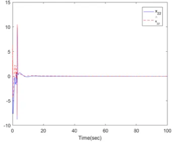
Figure 10. The trajectory of x22 for Example1
Figure 11. The trajectories of f1 and fˆ1 for Example 1
Figure 12. The trajectories of f2 and fˆ2 for Example 1
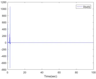
Figure 13. The control signal u t( ) for Example 1
( ( ))
D u t is an output of a dead zone, and
1
1( , )t 0.1x2( ) sint ( )t
δ x = , δ2(x, )t =0.1x22( ) sint ( )t are the disturbances.
In the simulation, parameters of the dead zone are 0.7
r
m = , ml =0.7, Ea =0.5, Eb=0.5. We select their bounds as mmax =1, mmin=0.5. Six fuzzy sets are defined over the interval [-3, 3] for xˆ11,xˆ12,xˆ21, and xˆ22, with labels NB, NM, NS, PS, PM, and PB, and their membership functions are
1 ˆ
( ) ,
ˆ 1 exp(5( 2)) NB ij
ij x
x
µ =
+ +
2
ˆ ˆ
( ) exp( ( 1.5) ),
NM xij xij
µ = − +
2
ˆ ˆ
( ) exp( ( 0.5) ),
NS xij xij
µ = − + (ˆ ) exp( (ˆ 0.5) ),2
PS xij xij
µ = − −
2
ˆ ˆ
( ) exp( ( 1.5) ), PM xij xij
µ = − − 1
ˆ
( ) ,
ˆ 1 exp( 5( 2)) PB ij
ij x
x
µ =
+ − −
where i=1, 2 , j=1, 2
Choose the sampling time as 0.01, and the observer gain as l11=1, l12=0.7 , l21=1, l22=0.7 . The initial values are chosen as x11(0)=3, x12(0)=1, x21(0)=3,
22(0) 1
x = , xˆ (0)11 =2.8 , xˆ (0)12 =0.9 , xˆ (0)21 =2.8 ,
22
ˆ (0) 0.9
x = , θˆf1(0)=0.18 , θˆf2(0)=0.18 , wˆ (0)1 =0 ,
ˆ(0) 0
h = , ˆ (0)ρ =0 , ˆ(0)η =0 , ˆ(0)φ =0 . The other parameters are selected as τ =1 , γf =0.7 , γ =h 4 ,
1 9
w
γ = , γρ =0.01, η=5. The simulation results are displayed by Figs. 3-14. Figs. 3-6 show the trajectories of the system states and their estimation states. Figs. 7-10 show the trajectories of the system state estimation errors. Figs. 11-12 show the trajectories of the system functions. Figs. 13-14 show the trajectories of the control signal u and the dead-zone input D u t( ( )).
5. Conclusions
An observer-based robust adaptive fuzzy control approach has been proposed in this paper for a class of uncertain underactuated systems in the presence of time delay and dead-zone input. The system states are assumed to be unmeasurable in this paper. With the help of fuzzy approximation, the fuzzy state observer has been constructed to estimate the unmeasurable states. Additionally, some adaptive laws are employed to estimate the unknown system parameters. The main contribution of this paper can be listed as follows: (i) the stability of the whole underactuated time-delay system has been proved via the Lyapunov-Krasovskii functional and (ii) all the signals of the closed-loop system are bounded by the presented control scheme. Finally, a series of simulation results have been presented to demonstrate the effectiveness of the proposed control approach.
REFERENCES
[1] N. Sun, T. Yang, Y. Fang, B. Lu and Y. Qian, "Nonlinear motion control of underactuated three-dimensional boom cranes with hardware experiments," IEEE Transactions on Industrial Informatics, vol. 14, no. 3, pp. 887-897, Mar. 2018.
[2] Z. Meng, D. V. Dimarogonas and K. H. Johansson, "Attitude coordinated control of multiple underactuated axisymmetric spacecraft," IEEE Transactions on Control of Network Systems, vol. 4, no. 4, pp. 816-825, Dec. 2017.
[3] A. Gutiérrez-Giles, F. Ruggiero, V. Lippiello and B. Siciliano, "Nonprehensile manipulation of an underactuated mechanical system with second-order nonholonomic constraints: The robotic hula-hoop," IEEE Robotics and Automation Letters, vol. 3, no. 2, pp. 1136-1143, Apr. 2018. [4] Y. Zhang, S. Li and X. Liu, "Adaptive near-optimal control
of uncertain systems with application to underactuated surface vessels," IEEE Transactions on Control Systems Technology, vol. 26, no. 4, pp. 1204-1218, Jul. 2018. [5] W. Gu, J. Yao, Z. Yao and J. Zheng, "Robust adaptive
control of hydraulic system with input saturation and valve dead-zone," IEEE Access, vol. 6, pp. 53521-53532, 2018. [6] H. Deng, J. Luo, X. Duan and G. Zhong, "Adaptive inverse
control for gripper rotating system in heavy-duty manipulators with unknown dead zones," IEEE Transactions on Industrial Electronics, vol. 64, no. 10, pp. 7952-7961, Oct. 2017.
[7] J. Yu, P. Shi, W. Dong and C. Lin, "Adaptive fuzzy control of nonlinear systems with unknown dead zones based on command filtering," IEEE Transactions on Fuzzy Systems, vol. 26, no. 1, pp. 46-55, Feb. 2018.
[8] Z. Liu, F. Wang, Y. Zhang, X. Chen and C. L. P. Chen, "Adaptive tracking control for a class of nonlinear systems with a fuzzy dead-zone input," IEEE Transactions on Fuzzy Systems, vol. 23, no. 1, pp. 193-204, Feb. 2015.
[9] L. Long and J. Zhao, "Adaptive fuzzy output-feedback control for switched uncertain non-linear systems," IET Control Theory & Applications, vol. 10, no. 7, pp. 752-761, Apr. 2016.
[10] H. Wang, B. Chen, X. Liu, K. Liu and C. Lin, "robust adaptive fuzzy tracking control for pure-feedback stochastic nonlinear systems with input constraints," IEEE Transactions on Cybernetics, vol. 43, no. 6, pp. 2093-2104, Dec. 2013.
[11] Q. Zhou, L. Wang, C. Wu, H. Li and H. Du, "Adaptive fuzzy control for nonstrict-feedback systems with input saturation and output constraint," IEEE Transactions on Systems, Man, and Cybernetics: Systems, vol. 47, no. 1, pp. 1-12, Jan. 2017. [12] Y. Gao, X. Sun, C. Wen and W. Wang, "Observer-based adaptive NN Control for a class of uncertain nonlinear systems with nonsymmetric input saturation," IEEE Transactions on Neural Networks and Learning Systems, vol. 28, no. 7, pp. 1520-1530, Jul. 2017.
[14] T. Wu, M. Karkoub, H. Wang, H. Chen and T. Chen, "Robust tracking control of MIMO underactuated nonlinear systems with dead-zone band and delayed uncertainty using an adaptive fuzzy control," IEEE Transactions on Fuzzy Systems, vol. 25, no. 4, pp. 905-918, Aug. 2017.
[15] H. Li, J. Wang, L. Wu, H. Lam and Y. Gao, "Optimal guaranteed cost sliding mode control of interval type-2 fuzzy time-delay systems," IEEE Transactions on Fuzzy Systems, vol. 26, no. 1, pp. 246-257, Feb. 2018.
[16] L. X. Wang, A Course in Fuzzy Systems and Control, Englewood Cliffs, NJ, USA: Prentice-Hall, 1997.