Parallel Numerical Solution of ABD and BABD linear systems arising from BVPs

Volume 10, Number 4, pp. 373–383. http://www.scpe.org c 2009 SCPE

PARALLEL NUMERICAL SOLUTION OF ABD AND BABD LINEAR SYSTEMS ARISING FROM BVPS∗

PIERLUIGI AMODIO†_{AND GIUSEPPE ROMANAZZI}‡

Abstract. We consider linear systems with coefficient matrices having the ABD or the Bordered ABD (BABD) structures. These systems arise in the discretization of BVPs for ordinary and partial differential equations with separated and non-separated boundary conditions, respectively. We describe the cyclic reduction algorithm for the solution of BABD linear systems which allowed us to write the codesBABDCRandGBABDCR(the latter code is suitable for matrices with a more generic BABD structure). A comparison of theGBABDCRcode with respect to the well-known sequential codeCOLROW on ABD linear systems is then analysed. We report some tests on an OpenMP Fortran 90 parallel version of theGBABDCRcode and finally we discuss about the use ofGBABDCRinside the BVP codeBVP SOLVER.

Key words: boundary value problems, ABD and BABD linear systems, parallel solution

1. Introduction. The discretization of Boundary Vale Problems for ordinary and partial differential equa-tions leads often to linear systems with Almost Block Diagonal (ABD) structure in case of separated boundary conditions, and Bordered ABD structure (BABD) in case of non-separated conditions (see [3, 18, 24]).

BABD linear systems

Ax=f (1.1)

have the coefficient matrixAwith the following sparsity structure

A=                             

Ba Bb

V1

V2

V3 V4

. .. . ..

VN

                            

. (1.2)

We recognize the boundary blocksBa andBb on the first row, and the block rowsVi which have some columns that overlap the blocks on the adjacent rows. For this reason, each blockVi can be represented as

Vi= Si₋1 Ti Ri , (1.3)

where the columns ofSi₋1 and Ri overlap columns of Vi−1 and Vi+1, respectively. Also V1 and VN have the

same structure in (1.3): the first columns of V1 (i. e., S0) are overlapped with those of Ba while the last columns ofVN (i. e., RN) are overlapped with those ofBb, see (1.2). We set the size of each blockVi equal to

ni×(mi−1+ki+mi), wheremi is the number of overlapped columns between the blocksVi andVi+1, andki

∗_{Work developed within the project “Numerical methods and software for differential equations”}

†_{Dipartimento di Matematica, Universit`a di Bari, Bari, Italy ([email protected])} ‡_{Departamento de Matem´atica, Universidade de Coimbra, Coimbra, Portugal (}

[email protected])

is the number of the non-overlapped columns ofVi; the size of the boundary blocksBa andBb isn0×m0 and

n0×mN, respectively. Since Ais a square matrix we have

N

X

i=0

ni=m0+

N

X

i=1

(mi+ki); (1.4)

it is also supposed thatN is much larger with respect to eachni,mi andki.

The ABD structure differs from the BABD structure for the presence of boundary blocks that have some null rows (the non-null rows of Ba correspond to null rows ofBb and viceversa). In this case it is preferable to refer toBa andBb as blocks of sizena×m0 andnb×mN, respectively. We impose then that no rows are overlapped betweenBa and Bb and we setn0=na+nb in (1.4). Moreover,Bb is located afterVN as the last block row so that the coefficient matrix can be represented as

A=                               

Ba

V1

V2

V3 V4

. .. . ..

VN

Bb

                              

. (1.5)

We note that ABD linear systems can be also solved by BABD solvers; this implies an higher computational cost and fill-in, see [24]. Conversely, a doubling of the size of each block is required for solving a BABD linear system using an ABD solver.

Since ABD linear systems are easier to solve than BABD systems, historically the former problem has received much more attention and several codes have been proposed. We quote the packageSOLVEBLOK [14] that uses Gaussian elimination with partial pivoting to ensure stability and requires fill-in. On the contrary, the packages COLROW and ARCECO in [15] are based on a modified version of Varah’s alternate row and column stable elimination [27] which exploits the structure of the ABD matrices to avoid fill-in. In particular, COLROW solves ABD linear systems with blocksVi of constant sizen×(2m+k), so that we haven=m+k

andni=n,mi=mandki=kfor eachi= 1, . . . , N.

Most nonlinear BVP packages employ ABD packages. The BVP codeCOLSYS [9] usesSOLVEBLOK to solve ABD linear systems arising from the use of orthogonal spline collocation (OSC) at Gauss points with B-spline bases. COLNEW [11] uses a modified version of SOLVEBLOK to solve ABD linear systems arising from the application of OSC at Gauss points with monomial spline bases. Both the Mono Implicit Runge Kutta (MIRK) code with defect control MIRKDC [17] and its new implementation BVP SOLVER [28] (the latter solves a wider class of BVPs with respect the former) use COLROW as solver for the obtained ABD systems. Modified versions of COLROW are used in the deferred correction code TWPBVP [13]. Other versions of COLROW are used in COLMOD [26], a modified version ofCOLNEW, and inACDC [12], that uses automatic continuation and OSC at Lobatto points to solve singularly perturbed BVODEs.

system is eight times larger with respect to the solution of an ABD linear system with blocks of the same size as the given BABD system.

The first available package for solving BABD systems is RSCALE; it is a shared memory parallel code used insidePMIRKDC [21], a parallel version ofMIRKDC. In [7, 8] the cyclic reduction algorithm is applied to the BABD matrix (1.2) with a simplified structure: the blocksSi and Ri are square of dimensionm and the blocksTiare null. This structure is also used byRSCALE. The coefficient matrix considered is then block lower bidiagonal with an additional block in the right-upper corner. The sequential codeBABDCR, introduced in [8] and available at the url

http://www.netlib.org/toms/859.

solves this kind of linear systems. Moreover, in [4] we have generalized the code BABDCR to solve BABD linear systems with the general structure (1.1)-(1.2) where each blockVi have sizen×(2m+k), withk >0 and

n=m+k. This latter code is calledGBABDCR and is available on the net at the url http://www.pitagora.dm.uniba.it/∼romanazzi/babdcr.html.

In [4, 5, 8, 24] BABDCR and GBABDCR have been compared to RSCALE and COLROW for solving BABD systems. The theoretical and numerical results show thatCOLROW has a computational cost which is till 3 times larger thanGBABDCR. This means that each code for BVPs with separated boundary conditions (for example,BVP SOLVER) usingCOLROW to solve the associated ABD linear systems, may be generalized to the solution of BVPs with non-separated boundary conditions by just replacing (the calls to) the linear solverCOLROW with GBABDCR. Moreover,BABDCR performs better (resulting faster and more precise) and has the same degree of parallelism with respect toRSCALE. Therefore, the efficiency ofPMIRKDC can be improved by replacingRSCALE with a parallel version of BABDCR.

This work originates from the observation that nowadays personal computers have motherboards with more CPUs (or core-processors), and this permits to overcome the physical limitations (such as speed and memory) of a single core-processor. Moreover these multi-core processors are easily accessible, and we can use them to speed-up the execution of each numerical code if the underlying algorithm is parallelizable. In our case, since cyclic reduction has an obvious parallel implementation, we can speed up the solution of ABD linear systems by implementingGBABDCR on such parallel architectures.

We propose, in fact, a shared memory implementation ofGBABDCRand compare it withCOLROW (that is not parallelizable) on multi-core computers. We believe that the replacement ofCOLROW in the existing (previously cited) BVODE packages with the parallel implementation of GBABDCR, can lead to a twofold advantage: the reduction of the computational cost when the code is run on multi-core processors, and the solution with no extra cost of BVODEs with non-separated boundary conditions.

The paper is organized as follows: in the next section we briefly sketch the cyclic reduction algorithm applied to general BABD linear systems, in Section 3 we explain the strategy used to parallelize the code on shared and distributed memory computers, and finally in the last section we compare the shared memory parallel implementation ofGBABDCRwithCOLROW in the solution of ABD systems and we discuss the performance ofBVP SOLVER whenGBABDCR replacesCOLROW.

2. The cyclic reduction algorithm. Let us rewrite the coefficient matrix (1.2)-(1.3) as

A=         

Ba Bb

S0 T1 R1

S1 T2 R2

S2 T3 R3

. ..

SN−1 TN RN

        

. (2.1)

In accordance with the structure of (2.1) we define the right hand side f of the linear system (1.1) as f =

fT

0 f1T . . . fNT

T

where eachfi is of lengthni, and the solution vector

x= zT

0 wT1 z1T . . . wTN−1 zTN

T ,

We solve the system (1.1) using a block cyclic reduction algorithm, that is, a recursive approach that reduces the original linear system to subsystems with a smaller number of unknowns. In this process the first and the last unknowns, z0 and zN, are always among the unknowns of the successive reduced systems; moreover, the first row containing the boundary blocks is unchanged in the reduction process. The boundary blocksBa and

Bb are then maintained in the first row of each reduction step.

Following [4], we consider a reduction step to eliminate, locally in each blockVi, the odd unknownswi of the solution vectorx. We observe that, sinceAis a non-singular matrix, the blocksTi of sizeni×ki, have full rankki because they are not overlapped by adjacentVi blocks. We may then compute the factorization:

e

PiTi= Lie_e

Gi ! e Ui= I e Fi I e

LiUie O

(2.2)

wherePie is a suitable permutation matrix,Lie and Uie are square matrices, andFie =Gie Le−1 i .

MultiplyingVi on the left byPie and the inverse of the lower triangular matrix in the last term of (2.2) we obtain

I −Fie I

e

Pi Si₋1 Ti Ri

= Sie−1 Lie Uie Rie

b

Si₋1 Rib

!

. (2.3)

Analogously, we perform the same operations on the right-hand sidefi, thus obtaining corresponding vectors ˜

fiandfibfor the right side. The row with the boundary blocks and the second row of (2.3) (for eachi= 1, . . . , N) give the linear system

       Ba Bb b

S0 R1b

b

S1 R2b

. .. . .. b

SN−1 RNb

              z0 z1 z2 .. . zN        =         f0 b f1 b f2 .. . b fN         . (2.4)

which has dimension equal to

N

X

i=0

mi =n0+

N

X

i=1

(ni−ki) and no longer depends on the unknownswi. These

unknowns will be computed in the last step of the back-substitution phase (when all thezi will be known), by using the first row of (2.3):

˜

LiUiwi˜ = ˜fi−Si˜₋1zi₋1−Rizi.˜

Factorization (2.3) does not require additional memory sinceFie may be saved together withLi andUiin place of Ti. Therefore, this first reduction should be considered as a (completely parallelizable) initial step to be applied to ABD or BABD matrices in order to simplify their structure.

Returning to the solution of (1.1), system (2.4) may be further on reduced by considering the cyclic reduction algorithm in [7, 8] (even if blocksSib andRib are not square). At first we compute the LU factorization of the (ni−ki+ni+1−ki+1)×mi matrix (of rankmi)

Pi Rib_b Si ! = Li Gi Ui= I Fi I LiUi O

that, applied to the block rows of indexiandi+ 1 in (2.4), gives

I −Fi I

Pi Sib−1 Rib

b

Si Ri+1b

! =

_¯

Si₋1 LiUi Ri¯ S′

i−1 R′i

. (2.5)

the first row in (2.5) may be used to computezi from zi−1 and zi+1. Factorization (2.5) requires additional

memory for the fill-in blocksFi.

Iterating this last step on the successively reduced systems we obtain, after⌈log2N⌉steps, a 2×2 block

(full) linear system

Ba Bb S∗

0 R∗N

z0 zN

=

f∗ 0 f∗ N

. (2.6)

The factorization and the solution of (2.6) gives the first and the last unknowns of the vectorx. Successively, a back substitution phase allows us to compute, in reverse order, all the other unknowns.

Ifmandkare constant (withn=m+k), the computational cost of this algorithm is

(14₃m3_{+ 4m}2_{k+ 2mk}2₊2

3k3)N. (2.7)

If k= 0 (all columns are overlapped), we have from (2.7) that the cost is 14 3m

3_{N as for the BABDCR}

algo-rithm, see [8]. The additional memory requirement (fill-in) is alwaysm2_{N (it does not depend onk) since the}

factorization of the blocksTiin (2.2) does not require fill-in.

The typical dimensions of the BABD linear system arising from BVPs consists of small dimensionsk, mof each row block, with respect to a large number of row blocksN.

In order to make a fair comparison, the computational cost ofCOLROW is

(5₃m3_{+ 4m}2_{k+ 3mk}2₊2

3k3+mnanb−(2m+k)kna)N, (2.8)

wherena andnb, withna+nb=m, denote the number of rows of the initial and of the final boundary block, respectively; remember thatCOLROW solves only ABD linear systems. Supposingna =nb =m/2, we have that GBABDCR costs at most 2.4 times more than COLROW and this ratio decreases whenk increases (if

k=mthe ratio is 1.4).

3. Parallel implementation. In this section we analyze and compare the main properties of parallel cyclic reduction algorithms written for shared and distributed memory architectures.

The cyclic reduction algorithm has a straightforward parallel implementation which has been described in several papers. See, for example, [1, 2, 6] where parallel cyclic reduction is used to solve tridiagonal systems and [5, 7, 24] where it is applied to BABD systems.

Let p the number of processors used1_{, the first phase of parallel reduction requires that each processor}

reduces a contiguous set of block rows, 

   

Si₋1 Ti Ri

Si Ti+1 Ri+1

. ..

Sj−1 Tj Rj

   

, (3.1)

to a single row

S∗ i₋1 R∗j

. (3.2)

In particular,q=N− ⌈N/p⌉pprocessors reduce ⌊N/p⌋block rows and the remainingp−q processors reduce

⌈N/p⌉block rows each. Note that, when qis non-zero, a different workload per processor is required.

At the end of this phase, each processor stores the block row (3.2) in the first and lastm2 _{locations of the}

assigned contiguous block rows (3.1) in place of Si−1 and Rj. The fill-in of these reductions is stored locally

in a private array of each processor, when a distributed memory architecture is used, or consists of contiguous blocks generated by each single processor, in case of a shared memory architecture.

Therefore, the first phase of reduction produces a reduced BABD system with coefficient matrix 

                

Ba Bb

V(1)

V(2)

. ..

V(p)

                 

, (3.3)

whereV(i) is computed by thei-th processor; this phase is then completely parallelizable.

Let us now analyze the parallel solution of the system with the coefficient matrix (3.3). Supposing, for sake of simplicity, that p is a power of 2, the parallel MPI algorithm (as in [7, 24, 5]), for a distributed memory architecture, requires log2p synchronizations, communications between processors, and reduction steps. On

shared memory architectures, clearly we do not require communications between processors because both the coefficient matrix and the right-hand side of the original system (1.1) are shared among processors. However, log2psynchronizations between processors are necessary.

This part of the algorithm determines, in both the architectures, the 2×2 block system (2.6). The solution of (2.6) is the only sequential part of the algorithm and is followed by the back-substitution phase which still has much parallelism inside.

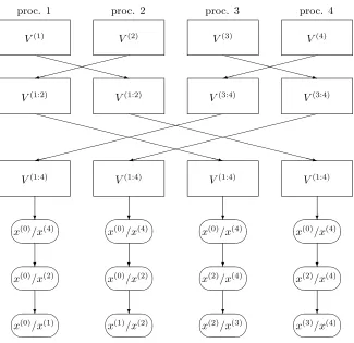
On a distributed memory architecture it is made possible that all the back-substitution phase requires no more synchronization or communication among the processors by considering bidirectional communications in the reduction phase (see Figure 3.1 and [6] for more details). This means that a copy of (2.6) is solved (concurrently) on all the processors.

On the other hand, on shared memory architectures, the number of processors is halved at each of the last log2p reduction steps and (2.6) is solved on a single processor. Then the number of processors is doubled for

the first log2psteps of back-substitution with a synchronization after each step.

In conclusion, if p≪ N the total operation count for each processor is essentially 1/p times the cost of (2.7). On shared memory architectures, the number of synchronizations is 2 log2p. The parallel code does not

require additional memory with respect to the sequential code and only a few local variables are needed on each processor. On distributed memory architectures, the number of synchronizations is only log2pbut each

processor needs to maintain log2pblocks of sizem×2mto avoid synchronization in the back-substitution and,

moreover, log2pcommunications ofm×2marrays and vectors of lengthmare necessary in the reduction phase.

Since distributed parallel architectures can have even hundreds processors, the main advantage of the parallel algorithm for these architectures is the possibility to strongly reduce the cost of the reduction and back-substitution phases by increasing the number of processors used. In such a case, however, a moderate overhead (of order log2N) appears due to the presence of synchronizations and communications.

As already mentioned, shared memory architectures are nowadays much easier to access. They have a limited number of processors (up to 4 in our tests), but the parallel algorithms for these architectures have a double advantage: there is no need to send the initial data to the local memory of each processor and there is no large communication step after each synchronization. This means that, for a given number of processors, these algorithms can lead to a better speed-up than that observed on distributed memory architectures.

4. Numerical results. In this section we report some numerical tests to compare COLROW with the shared memory (OpenMP) parallel version of GBABDCR (here called GBABDCR OMP) in the solution of ABD systems on multi-core computers. Our aim is to stress thatGBABDCR OMP may be efficiently employed in each BVP solver that requires the solution of ABD/BABD systems on the new multi-core personal computers. For this reason we analyze the execution times of sequential runs performed on an alpha EV6.7 (21264A, 667 MHz) and of parallel runs performed on an Intel Core 2, Quad CPU Q9550, (2.83 GHz) multi-processor with 4 cores. We consider ABD linear systems with blocks of the same size and with the same overlap (mi=m,

proc. 1 proc. 2 proc. 3 proc. 4

V(1) _V(2) _V(3) _V(4)

X_X X_X X_X X_X X z 9 X_X X_X X_X X_X X z 9

V(1:2) _V(1:2) _V(3:4) _V(3:4)

X_X X_X X_X X_X X_X X_X X_X X_X

XXz

X_X X_X X_X X_X X_X X_X X_X X_X

XXz 9 9

V(1:4) _V(1:4) _V(1:4) _V(1:4)

? ? ? ?

x(0)/x(4)

x(0)/x(4)

x(0)/x(4)

x(0)/x(4)

? ? ? ?

x(0)_/x(2)

x(0)_/x(2)

x(2)_/x(4)

x(2)_/x(4)

? ? ? ?

x(0)_/x(1)

x(1)_/x(2)

x(2)_/x(3)

x(3)_/x(4)

Fig. 3.1_{.Communications among processors on a distributed memory architecture with}p= 4.

In Tables 4.1 and 4.2 we compare the elapsed time of some GBABDCR and COLROW runs using the sequential computer to estimate the theoretical operation counts. We observe that, fork= 0 the ratio between the elapsed time of GBABDCR and COLROW decreases from 3.26 to 2.32 (the expected value is 2.4) as we increasenwhile fork =m the ratio decreases from 4.75 to 1.64 (the expected value is 1.4). A reason of this strange behaviour is due to the large use inGBABDCR of BLAS3 routines [16] (such as DGEMM, DTRSM) which have poor performance for small matrices (see tests in [22, 23]) and make this algorithm more efficient for largekand monly.

Table 4.1

Elapsed times (in seconds) of GBABDCR and COLROW for solving ABD linear systems withN= 10000and variablen=m

(k= 0)

n GBABDCR COLROW GBABDCR/COLROW

4 0.0795 0.0244 3.2600

8 0.2525 0.0947 2.6675

12 0.5768 0.2294 2.5149

16 1.0753 0.4377 2.4565

20 1.6946 0.7291 2.3243

These results show therefore that, for small size n of each block, it is quite difficult that GBABDCR overcomes the performance ofCOLROW on parallel machines. Effectively forn <8 we were not able to lower COLROW timings by usingGBABDCR OMP on 4 cores.

In Tables 4.3-4.6 we show the performance ofGBABDCR OMP running on shared memory architectures forN= 10000,20000,40000 andn= 8,16.

Table 4.2

Elapsed times of GBABDCR and COLROW for solving ABD linear systems withN= 10000and variablen= 2m(k=m)

n GBABDCR COLROW GBABDCR/COLROW

4 0.0986 0.0207 4.7529

8 0.1840 0.0712 2.5822

12 0.3582 0.1940 1.8465

16 0.5558 0.3235 1.7179

20 0.9118 0.5546 1.6441

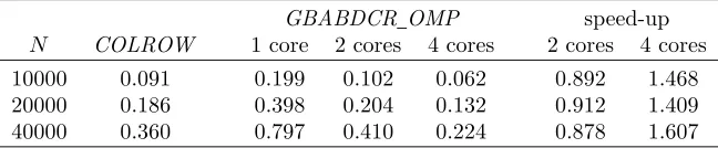
Table 4.3

Elapsed times of GBABDCR OMP and COLROW on a quad-core machine for ABD linear systems withn=m= 8(k= 0) and variableN. Speed-up is computed as the ratio between the elapsed time of COLROW and GBABDCR OMP

GBABDCR OMP speed-up

N COLROW 1 core 2 cores 4 cores 2 cores 4 cores

10000 0.091 0.199 0.102 0.062 0.892 1.468

20000 0.186 0.398 0.204 0.132 0.912 1.409

40000 0.360 0.797 0.410 0.224 0.878 1.607

a multicore architecture, we can effectively speed-up the performance of any BVP solver when the size of the problem is sufficiently large, just replacingCOLROW withGBABDCR OMP. Since a code for BABD systems may be directly applied to ABD systems, the modifications in the code are limited to a few instructions.

In particular, in BVP SOLVER we have inserted a subroutine that creates the non-separated boundary blocks of the linear system starting from the given separated boundary conditions and we have added a fill-in vector which is only required by GBABDCR OMP. We point out that in BVP SOLVER the resulting linear systems have a BABD structure withk= 0 andm=n.

As an example, we have considered the solution of a 8×8 nonlinear system of equations describing fluid injection through one side of a long vertical channel (see [10, Example 1.4]). We have taken into account this problem with the following parameters

R= 1000, P = 0.7∗R, METH = 2

and fixed equal to 1 both the initial guess for the solution and the unknown parameterA.

Table 4.7 shows the results obtained by setting the exit tolerance equal to 10−6_{, 10}−7 _{and 10}−8_{. A few}

comments need to be done on this example. The number of requested linear system solutions (SOLV) is about 8 times the number of factorizations (FACT). Since this size of the ODE is justn= 8 and in any ABD/BABD code the computational cost of the factorization phase (FACT) is about n times that of the solution phase (SOLV), then we expect the execution time of the two phases to be approximately equivalent.

From Table 4.7 we observe that the percentage of time required by SOLV usingGBABDCR is higher than that requested by FACT (the opposite happens when we use COLROW) and it is therefore difficult to obtain a large speed-up with the replacement of the linear algebra solver. By considering only the linear algebra part (see % LIN ALG in the table) ofBVP SOLVER,GBABDCR reduces its elapsed time of a factor in the range [1.5, 1.7] when we use 4 cores instead of 1. This is anyway sufficient to obtain on 4 cores an execution faster thanCOLROW.

We have to specify that on BVPs of size smaller than 8 we were not able to improve timings obtained with COLROW. The size of the considered problem is anyway small, and this implies two negative aspects: linear algebra is not the most time consuming part of the algorithm and, for such small dimensions, COLROW is much better than GBABDCR. Nevertheless, it is clear that parallelism is really more useful to reduce timing in presence of very large nonlinear BVPs.

Table 4.4

Elapsed times of GBABDCR OMP and COLROW on a quad-core machine for ABD linear systems withn=m= 16(k= 0) and variableN. Speed-up is computed as the ratio between the elapsed time of COLROW and GBABDCR OMP

GBABDCR OMP speed-up

N COLROW 1 core 2 cores 4 cores 2 cores 4 cores

10000 0.584 1.038 0.525 0.299 1.112 1.953

20000 1.174 2.054 1.049 0.552 1.119 2.127

40000 2.332 4.131 2.098 1.092 1.112 2.136

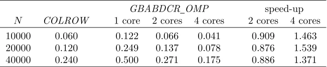
Table 4.5

Elapsed times of GBABDCR OMP and COLROW on a quad-core machine for ABD linear systems withn= 2m= 8(k=m) and variableN. Speed-up is computed as the ratio between the elapsed time of COLROW and GBABDCR OMP

GBABDCR OMP speed-up

N COLROW 1 core 2 cores 4 cores 2 cores 4 cores

10000 0.060 0.122 0.066 0.041 0.909 1.463

20000 0.120 0.249 0.137 0.078 0.876 1.539

40000 0.240 0.500 0.271 0.175 0.886 1.371

used. Finally, we emphasize that the performance ofBVP SOLVERcan be further improved withGBABDCR, by considering that the original problem has three nonseparated boundary conditions and, therefore, it can be recast so that a 18×18 BABD linear system is obtained.

REFERENCES

[1] P. Amodio, L. Brugnano. Parallel factorizations and parallel solvers for tridiagonal linear systems.Linear Algebra Appl.172, 347–364, 1992.

[2] P. Amodio, L. Brugnano, T. Politi. Parallel factorizations for tridiagonal matrices.SIAM J. Numer. Anal.30, 813–823, 1993. [3] P. Amodio, J. R. Cash, G. Roussos, R. W. Wright, G. Fairweather, I. Gladwell, G. L. Kraut and M. Paprzycki. Almost block diagonal linear systems: sequential and parallel solution techniques, and applications. Numer. Linear Algebra Appl.7, no. 5, 275–317, 2000.

[4] P. Amodio, I. Gladwell and G. Romanazzi. Numerical solution of general Bordered ABD linear systems by cyclic reduction. J. Numer. Anal., Industrial and Applied Mathematics 1, no. 1, 5–12, 2006.

[5] P. Amodio, I. Gladwell and G. Romanazzi. An algorithm for the solution of Bordered ABD linear systems arising from Boundary Value Problems.Multibody Dynamics 2007, ECCOMAS Thematic Conference, C. L. Bottasso, P. Masarati, L. Trainelli (eds.), Milano (Italy), June 25–28, 2007.

[6] P. Amodio, N. Mastronardi. A parallel version of the cyclic reduction algorithm on a Hypercube.Paral. Comput.19, 1273– 1281, 1993.

[7] P. Amodio and M. Paprzycki. A cyclic reduction approach to the numerical solution of boundary value ODEs.SIAM J. Sci. Comput.18, no. 1, 56–68, 1997.

[8] P. Amodio and G. Romanazzi. BABDCR: a Fortran 90 package for the solution of Bordered ABD systems.ACM Trans. Math. Software 32, no. 4, 597–608, 2006. (Available on the web address “http://www.netlib.org/toms/859”)

[9] U. M. Ascher, J. Christiansen and R.D. Russell. Algorithm 569: COLSYS: Collocation Software for Boundary-Value ODEs. ACM Trans. Math. Software 7, no. 2, 223–229, 1981.

[10] U. M. Ascher, R.M.M. Mattheij, and R.D. Russell. Numerical Solution of Boundary Value Problems for Ordinary Differential Equations. SIAM Classics In Applied Mathematics, 1995.

[11] G. Bader and U. Ascher. A new basis implementation for a mixed order boundary value ODE solver.SIAM J. Sci. Statist. Comput.8, no. 4, 483–500, 1987.

[12] J. R. Cash, G. Moore and R.W. Wright. An automatic continuation strategy for the solution of singularly perturbed nonlinear boundary value problems.ACM Trans. Math. Software27, no. 2, 245–266, 2001.

[13] J. R. Cash and R. W. Wright. A deferred correction method for nonlinear two-point boundary value problems: Implementations and numerical evaluation.SIAM J. Sci. Statist. Comput.12, no. 4, 971–989, 1991.

[14] C. De Boor and R. Weiss. SOLVEBLOK: A package for solving almost block diagonal linear systems.ACM Trans. Math. Software 6, no. 1, 80–87, 1980.

[15] J. C. Diaz, G. Fairweather and P. Keast. FORTRAN packages for solving certain almost block diagonal linear systems by modified alternate row and column elimination.ACM Trans. Math. Software9, no. 3, 358–375, 1983.

[16] J. J. Dongarra, J. Du Croz, I. S. Duff and S. Hammarlin, Algorithm 679: A set of Level 3 Basic Linear Algebra Subprograms, ACM Trans. Math. Software 16, 18–28, 1990.

[17] W. H. Enright and P. H. Muir. Runge-Kutta software with defect control for boundary value ODEs.SIAM J. Sci. Comput.

Table 4.6

Elapsed times of GBABDCR OMP and COLROW on a quad-core machine for ABD linear systems with n = 2m = 16 (k=m) and variableN. Speed-up is computed as the ratio between the elapsed time of COLROW and GBABDCR OMP

GBABDCR OMP speed-up

N COLROW 1 core 2 cores 4 cores 2 cores 4 cores

10000 0.370 0.468 0.253 0.145 1.463 2.552

20000 0.742 0.938 0.506 0.278 1.466 2.669

40000 1.485 1.875 0.977 0.552 1.520 2.690

Table 4.7

Total elapsed times of BVP SOLVER using COLROW and GBABDCR OMP as linear algebra solver on a nonlinear8×8 BVP.# FACTand# SOLVdenote, respectively, the number of linear system factorizations and solutions performed by the code. % FACTand% SOLV denote, respectively, the percentage of the total elapsed time required by linear system factorizations and solutions in BVP SOLVER.% LIN ALG = % FACT + % SOLVdenotes the percentage of the total elapsed time required by the linear algebra part.

TOL 1e-8 1e-7 1e-6

Nmax 63357 19281 6466

# FACT 21 20 20

# SOLV 170 161 151

COLROW 30.886 3.409 0.895

% FACT 5.83% 14.66% 21.16%

% SOLV 2.73% 9.20% 17.19%

% LIN ALG 8.56% 23.86% 38.35%

GBABDCR (1 core) 31.831 3.737 1.067

% FACT 6.86% 14.84% 21.60%

% SOLV 5.42% 16.80% 29.56%

% LIN ALG 12.28% 31.64% 51.16%

GBABDCR (2 cores) 30.881 3.435 0.917

GBABDCR (4 cores) 30.484 3.260 0.846

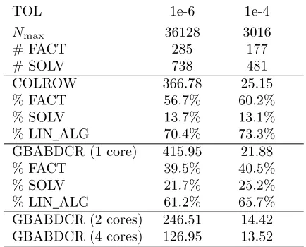
Table 4.8

Total elapsed times of BVP SOLVER using COLROW and GBABDCR OMP as linear algebra solver on a nonlinear21×21 BVP.# FACTand# SOLVdenote, respectively, the number of linear system factorizations and solutions performed by the code. % FACTand% SOLV denote, respectively, the percentage of the total elapsed time required by linear system factorizations and solutions in BVP SOLVER.% LIN ALG = % FACT + % SOLVdenotes the percentage of the total elapsed time required by the linear algebra part.

TOL 1e-6 1e-4

Nmax 36128 3016

# FACT 285 177

# SOLV 738 481

COLROW 366.78 25.15

% FACT 56.7% 60.2%

% SOLV 13.7% 13.1%

% LIN ALG 70.4% 73.3%

GBABDCR (1 core) 415.95 21.88

% FACT 39.5% 40.5%

% SOLV 21.7% 25.2%

% LIN ALG 61.2% 65.7%

GBABDCR (2 cores) 246.51 14.42

[18] G. Fairweather and I. Gladwell. Algorithms for almost block diagonal linear systems.SIAM Rev.46, no. 1, 49–58, 2004. [19] B. Garrett and I. Gladwell. Solving bordered almost block diagonal systems stably and efficiently.J. Comput. Methods Sci.

Engrg.1, 75–98, 2001.

[20] K. R. Jackson and R. N. Pancer. The parallel solution of ABD systems arising in numerical methods for BVPs for ODEs. Techinical Report n. 255/91, Computer Science Department, University of Toronto, 1992.

[21] P. H. Muir, R. N. Pancer and K.R. Jackson. PMIRKDC: a parallel mono-implicit Runge-Kutta code with defect control for boundary value ODEs.Paral. Comput.29, 711–741, 2003.

[22] J. R. Herrero and J. J. Navarro. Improving Performance of Hypermatrix Cholesky Factorization. In9th International Euro-Par Conference, 461–469, August 2003.

[23] A. Rem´on, E. S. Quintana-Ort´ı and G. Quintana-Ort´ı. Cholesky factorization of band matrices using multithreaded BLAS. In B. K˚agstr¨om, E. Elmroth, J. Dongarra, J. W´asniewski, eds., PARA 2006. Lect. Notes Comp. Sci. 4699, 608–616. Springer, Heidelberg.

[24] G. Romanazzi. Numerical Solution of Bordered Almost Block Diagonal linear systems arising from BVPs. Ph.D. Thesis, Universit`a di Bari, 2006.

[25] M. Snir, S.W. Otto, S. Huss-Lederman, D. Walker and J. Dongarra.MPI: The Complete Reference.The MIT Press, Cam-bridge, Massachusetts, 1996.

[26] R. W. Wright, J. Cash and G. Moore. Mesh selection for stiff two-point boundary value problems.Numer. Algorithms 7, 205–224, 1994.

[27] J. M. Varah. Alternate row and column elimination for solving certain linear systems. SIAM J. Numer. Anal.13, 71–75, 1976.

[28] L. F. Shampine, P. H. Muir and H. Xu. A User-Friendly Fortran BVP Solver. J. Numer. Anal. Ind. and Appl. Math.11, no. 2, 1201–217, 2006